Molecular simulation of protein-surface interactions: Benefits, problems, solutions, and future directions (Review)

Abstract

While the importance of protein adsorption to materials surfaces is widely recognized, little is understood at this time regarding how to design surfaces to control protein adsorption behavior. All-atom empirical force field molecular simulation methods have enormous potential to address this problem by providing an approach to directly investigate the adsorption behavior of peptides and proteins at the atomic level. As with any type of technology, however, these methods must be appropriately developed and applied if they are to provide realistic and useful results. Three issues that are particularly important for the accurate simulation of protein adsorption behavior are the selection of a valid force field to represent the atomic-level interactions involved, the accurate representation of solvation effects, and system sampling. In this article, each of these areas is addressed and future directions for continued development are presented.

I. Introduction

As widely recognized, the adsorption of proteins to synthetic material surfaces is of great importance in the field of biomaterials because of its governing role in determining cellular responses to implanted materials and substrates for tissue engineering and regenerative medicine.^1–5 Cells, of course, generally do not have receptors for synthetic polymers, metals, or ceramics, and thus lack any means of responding to macroscopically sized, chemically stable material surfaces. However, when a material is exposed to a protein-containing solution, proteins rapidly adsorb onto the surface, thus rendering it bioactive, and it is the bioactive state of these adsorbed proteins that drive cellular response.^1,5 The effects of adsorption on the bioactive state of proteins are also of critical importance in many other applications, such as the development and optimization of surfaces for biosensors,^6,7 bioactive nanoparticles,^8–12 biocatalysis,^13–16 bioanalytical systems for diagnostics and detection,^17–22 and bioseparations.^13,15,23

Because of its importance, protein adsorption behavior has been intensively studied over the past several decades. While much has been learned from these efforts, a detailed understanding of the molecular mechanisms underlying protein adsorption behavior and how to control it is still lacking, which means that the design of surfaces for biomedical and biotechnology applications can, at best, only be approached by educated trial-and-error methods. However, because the number of degrees of freedom involved for surface design is so enormously large (e.g., types of functional groups present, their spatial distribution, and surface topology), the chance of finding optimal conditions to control protein adsorption behavior by a trial-and-error approach for a given application is infinitesimally small. Given this situation, it is clear that new approaches are needed to help understand protein adsorption behavior at the molecular level, so that this understanding can then be applied to guide surface design to directly control these types of interactions.

One of the most direct methods of addressing interactions at the molecular level is through molecular simulation. While this has had relatively very little impact in the biomaterial field at this time, molecular simulation is considered to be an essential technology in other areas, such as for the understanding of protein folding,^24–31 protein-protein^32–37 and protein-cell membrane^38–40 interactions, and drug design.^41–45 Similar potential exists for the application of molecular simulation methods to help understand protein adsorption behavior. However, as with other areas of application, molecular simulation methods cannot just be borrowed, but must be carefully and specifically developed, validated, and applied for this particular application.

This article is intended to help provide direction for the biomaterial field as it takes on the challenge of developing molecular simulation methods for its own applications. The specific objectives of this article are threefold: (1) to provide a general introduction to molecular simulation methods for the biomaterial field, (2) to highlight the key factors and problems involved in the application of molecular modeling methods for the simulation of protein adsorption behavior, and (3) to present approaches to address these problems so that these types of simulations can be conducted in a manner that will provide meaningful results.

II. Types of Molecular Simulation Methods

Molecular simulation methods can be divided into three distinct classes based on the degree of molecular detail that is explicitly addressed in the simulation and the manner in which the potential energy of the molecular system is calculated. These three classes are quantum mechanical (QM) methods, all-atom empirical force field methods, and united-atom (or coarse-grained) methods.⁴⁶ The latter two classifications can each be subdivided into three different methods, namely, molecular mechanics (MM), Monte Carlo (MC), and molecular dynamics (MD). These three methods employ three different types of mathematical approaches to calculate properties of the system, namely, energy minimization, integration over configurational phase space, and solution of Newton equations of motion, respectively.

QM methods utilize various means to approximately solve the Schrödinger equation to calculate the properties of a molecular system using electrons as the fundamental particles under consideration. These types of calculations can be highly accurate and require no fitted parameters, but they are also extremely computationally expensive. Because these methods are so computationally intense, at this time they are generally restricted to no more than a few tens of atoms, and when used for MD simulations, they are restricted to a few picoseconds in time scale. Despite these limitations, because of their high level of accuracy, these methods are very useful for evaluating atomic-level interactions and are widely used to develop parametrization for the all-atom empirical force field methods.

All-atom empirical force field methods do not address the behavior of electrons, but rather treat individual atoms as the fundamental unit and use an empirically fit force field equation to calculate the amount of energy involved in atom-atom interactions based on the configuration of the atoms and their state of bonding. Force field methods are commonly used for MM, Metropolis MC, and MD simulations.⁴⁶ Because these calculations are much less rigorous than QM calculations, all-atom empirical force fields can be relatively easily used to model the behavior of systems with tens of thousands of atoms, and when used for MD simulations, can relatively easily simulate time frames for tens of nanoseconds. At this time, these methods are thus applicable to address the behavior of peptide-surface interactions and protein-surface interactions for small proteins. Another specific advantage of the ability to treat large systems of atoms with these types of methods is that aqueous solvation effects can be directly addressed by explicitly representing water molecules and ions in solution, thus enabling solvent molecules to be directly represented as a dynamic, interactive part of the molecular system. These methods are also particularly valuable in that they can be used to calculate differences in free energy, which is of fundamental importance for understanding and predicting protein adsorption behavior.

The third type of molecular simulation, united-atom or coarse-grained methods, treats groups of atoms as the fundamental unit in the system, with a force field equation then used to define energy contributions as a function of the configuration of the united-atom elements with respect to one another and their connectivity with one another. Generally these methods treat solvation effects implicitly by using some type of mean-field approximation. Both of these types of approximations greatly reduce the computational cost of the system, thus enabling system size, conformational searching, and time scales to be greatly expanded, with this advantage coming at a cost of decreased accuracy.

III. Key Factors for the Molecular Simulation of Peptide/Protein-Surface Interactions

Of the three basic classes of molecular simulation methods, the one most directly applicable for the simulation of peptide-surface or protein-surface interactions is the class of methods that uses an all-atom empirical force field. If properly parametrized and applied, these methods can accurately represent the atomic-level behavior for a system containing a sufficiently large numbers of atoms to represent an adsorbent surface, peptides or a small protein, and the water and ions of the solvent.

The key phrase in the preceding sentence is “if properly parametrized and applied.” There are three main issues that must be appropriately addressed in order to perform a useful molecular simulation of peptide-surface interactions. The first is force field parametrization. The force field equation determines how atoms interact with one another during a simulation, and the accuracy of a simulation depends directly on the suitability of the set of force field parameters that are used to represent the types of atom-atom interactions involved. The second key issue pertains to how solvation effects are accounted for. If solvent molecules are explicitly included in the molecular system being evaluated, then this relates directly to the previous issue, namely, force field parametrization to accurately represent the molecular-level behavior of water and ions in solution. Alternatively, if the solvent is represented using some type of mean-field approximation, as with implicit solvation methods, then the accuracy of this approximation must be considered. The third key issue is related to system sampling and what is called sampling ergodicity. In practical terms, sampling ergodicity refers to the need to sample a sufficient number of configurational states of a system in order to calculate a representative ensemble-average property of the system, such as the average potential energy or change in free energy for a given process. This becomes problematic when different states of the system are separated by relatively high energy barriers, which tend to trap the system in localized areas, thus preventing other important states from being sampled. When this occurs, it results in errors in the calculated properties of the system. Each of these key area is addressed more thoroughly in the following sections.

IV. Empirical Force Field Parametrization

The key component of an all-atom empirical force field method, whether it be MM, MC, or MD, is the parametrization of the force field. The force field equation is actually a relationship that describes how the potential energy of the system changes as a function of the positions of the atoms for a given state of atomic bonding. It is called a force field equation because when differentiated with respect to a spatial coordinate, the resulting expression provides the forces acting on each atom as a function of their relative positions. These atomic forces are used in MM calculations to determine how the arrangement of atoms in the system can be adjusted to minimize its energy, and in MD simulations to determine how atoms should move over a given time step of the simulation. In MC simulations, the force field equation is directly used to calculate the potential energy of the system as a function of the atomic positions, and the change in potential energy as a function of changes in atomic coordinates is then used as a means to explore the conformational space of the system. Although special types of force fields have been developed to enable covalent bond forming and breaking,^47–49 generally empirical force field methods do not allow the bonded state of the system to change during a simulation. Thus, for a given state of bonding, the potential energy of the system is completely determined by the respective coordinate positions of the atoms within the system.

As its name implies, the parameters of an empirical force field are empirically determined for a given set of atoms for a designated type of application. There are primarily two types of empirical force fields that are used for molecular simulations, which are referred to as class I force fields [e.g, AMBER,^50,51 CHARMM,^52,53 OPLS,^54,55 GROMOS (Refs. 56 and 57)] and class II force fields [e.g., MM2–4,^58–60 CFF,⁶¹ PCFF,^62–64 COMPASS (Refs. 65–67)]. Both class I and II force fields have parameters that represent potential energy contributions for bonded interactions in the form of separate terms for covalent bond stretching, bond bending, and bond rotation, and nonbonded interactions in the form of both electrostatic and Lennard-Jones interactions. For the bonded terms, force field parameters are used to define a zero energy position for bond length, bond angle, and dihedral angle and to set force constants that represent how potential energy increases as a given bonding condition shifts away its zero-position value. Nonbonded electrostatic interactions are represented by Coulomb's law, thus requiring only one force field parameter for each atom type as defined by its bonded state (e.g., carbonyl carbon atom versus aliphatic carbon atom), which designates its partial charge. The nonbonded Lennard-Jones term of the force field, on the other hand, requires two parameters per atom type; one that defines the van der Waals radius of the atom and the other its contribution to the potential energy well depth when it interacts with another atom. The class II force field expression is much more complex than the class I force field in that it includes higher-order terms for the energy contributions for bond stretch, bend, and dihedral rotations, and it includes cross terms that address how one type of bonding condition influences another, such as how bond stretching influences bond bending and dihedral rotations. Class I force fields are typically used for the simulation of biomolecules (e.g., proteins, DNA, RNA, carbohydrates) in aqueous solution because they provide an acceptable level of accuracy while being very computationally efficient,⁶⁸ while class II force fields are typically used for the simulation of small molecules in vacuum and bulk synthetic materials (polymers, metals, and ceramics), with the higher-order terms and cross terms used as necessary to adequately represent the molecular behavior of the system.⁶¹ The values of the bonded parameters and the atomic partial-charge parameters for these force fields are typically determined from quantum mechanical calculations, while the Lennard-Jones parameters may be determined either by quantum mechanical calculations or are adjusted to match experimental data, such as heats of vaporization, heats of solvation, and liquid density.^53,68,69 The Lennard-Jones terms are particularly subject to error because they are generally developed for individual atom types, with arithmetic or geometric combining rules then used to provide the equilibrium separation distance and well-depth characteristics for pairing one atom type with another.

One of the inherent difficulties with empirical force field methods is that the actual partial charge of a given atom in a molecular system depends not only on the types of atoms to which it may be covalently bonded but also on the types of atoms immediately surrounding it and the polarizability of the atom in question and those in its immediate surroundings. Thus, while a quantum mechanical simulation of a given molecular system will automatically adjust the effective partial-charge state of each atom in the system as a function of its local environment by the calculation of electronic orbital wave functions and energies, an empirical force field uses predefined fixed partial charges for designated atoms as a function of their state of covalent bonding. The designated partial-charge values of the atoms, of course, then do not change in response to the surrounding conditions, thus leading to potential errors in the simulated behavior of the system. Although attempts are currently underway by many groups to develop polarizable empirical force field methods that enable partial charges to adjust to their local surroundings during a simulation,^70–73 these methods are still not widely used, primarily because of the high computational cost involved.⁷⁴

Because of the restriction to use fixed partial charges and other fixed parameters for a molecular simulation, empirical force fields are generally not broadly transferable. This means that force field parameters that are developed for one set of conditions, such as peptide folding in aqueous solution, are generally not suitable for the same general set of functional groups under a different set of conditions, such as for a bulk solid-phase polymer or the adsorption of a protein to a polymer surface. This issue was very clearly demonstrated in a paper by Oostenbrink et al.,⁷⁵ in which two different sets of partial-charge parameters were needed to accurately represent the behavior of the same set of molecules in their pure condensed liquid state versus when represented in aqueous solution.

Because of this problem, it is generally acknowledged that force field parameters must be validated for each different type of application because subtle differences in the molecular conditions of a system can substantially influence the behavior of the atoms in the system. This issue is extremely pertinent for the simulation of peptide-surface interactions. While at first glance it seems very reasonable that force field parametrization that has been validated for peptide folding in aqueous solution should be perfectly suitable to be used to represent peptide adsorption behavior to a functionalized surface, there are sufficient differences between these two types of processes that suggest that this might not be the case. Peptide folding behavior is largely influenced by the covalent bonding state of the peptide chain, with nonbonded interactions playing a very important but secondary role due to the fact that nonbonded interactions (i.e., electrostatic and Lennard-Jones interactions) are much weaker than covalently bonded interactions (i.e., covalent bond stretching, bending, and dihedral rotations). In contrast to this, peptide adsorption behavior is completely driven by nonbonded interactions and, most importantly, it is dominated by the relative strength of the nonbonded interactions of the atoms of the peptide versus atoms of the solvent for the atoms of the adsorbent surface. Thus while small errors in the partial-charge state and Lennard-Jones parameters of the atoms of a peptide may result in negligible errors in the manner in which it folds in aqueous solution, these same small errors may introduce large errors in the manner in which it adsorbs to a surface. This situation is further exacerbated by the fact that partial charges are not able to adjust to their local environment, which is likely to change at the interphase region of a multiphase system, and Lennard-Jones interactions may be particularly subject to error when calculated between mixed atom types in separate phases of a multiphase system.

For this reason, it is extremely important that force field parameters that are borrowed from one application and applied to another (i.e., borrowed from a protein folding force field to simulate protein adsorption behavior) be critically evaluated for the new situation. This enables possible errors in the parametrization to be identified, appropriately modified, and then validated for use for the intended application. If this is not done, then little confidence can be placed in the simulation results.

Figure 1 shows an example of how an imbalance in force field parameters can result in an error in the simulated behavior. In this case, an oligo(ethylene-oxide)-functionalized surface was predicted to strongly adsorb peptides,^76,77 which is contrary to well established experimental behavior for this type of surface chemistry.⁷⁸

Fig. 1.

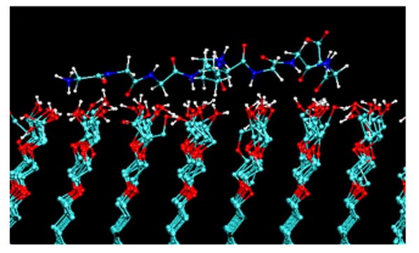
A snap shot from a molecular dynamics simulation of a G₄-K-G₄ peptide over an oligo(ethylene-oxide)-SAM surface [OEG, functional group structure: (-O-CH₂-CH₂)₂-OH)] using the default gromacs force field parameters (Ref. 138). The peptide strongly adsorbed to the OEG surface via a combination of hydrogen bonds with the OH groups at the end of the OEG chains and hydrophobic interactions between CH₂ groups of the peptide and the ethylene segments of the OEG chains. Experimental studies show this type of surface to be very nonadsorbing for peptides and proteins (Ref. 78) This simulation thus demonstrates an example where the force field parameters are not properly tuned to represent realistic adsorption behavior. Adapted from Ref. 76; used with permission.

Of course, in order to evaluate, modify, and validate a given set of force field parameters for a given application, it is necessary to know what the correct behavior of the system is so that the simulation results can be critically evaluated. This is particularly problematic for the case of peptide adsorption behavior because at this time there are little experimental data that designate what a properly parametrized force field should predict in terms of peptide adsorption behavior.

To address this critical issue, my research group has spent the past several years developing methods to both experimentally determine the standard state free energy of peptide-surface interactions^79,80 and to calculate changes in adsorption free energy by molecular simulation using an all-atom empirical force field^76,77,81 so that the accuracy of force field parameters can be critically assessed. These methods are now being applied to experimentally characterize the adsorption behavior of a large library of peptide-surface combinations using a host-guest peptide model with varied guest amino acid residues and alkanethiol self-assembled monolayer (SAM) surfaces with surface functionality selected to represent a wide variety of functional groups commonly found in polymers. In addition, the developed molecular simulation methods are being applied to calculate the change in free energy for peptide adsorption for these same systems using the CHARMM force field.^52,53 By comparing the simulation results to the experimental results, which represents an ongoing effort, we will have a basis for evaluating how well the CHARMM force field is able to represent the interactions between amino acid residues and polymerlike functional groups in an aqueous environment. These comparisons will then be used to identify problems with the existing parametrization for this application. This will provide a basis from which the parametrization for water-surface and peptide-surface interactions can be adjusted and properly balanced to optimize agreement with experimental results, thereby establishing a validated empirical force field for amino acid residue-surface interactions. Although this represents a very large undertaking, this degree of effort is deemed to be necessary in order to provide a sufficient level of confidence that these types of molecular simulations will accurately reflect actual peptide adsorption behavior.

The exciting aspect of the development of an empirical force field for amino acid residue-surface interactions is the fact that all proteins are essentially composed of the same set of 20 naturally occurring amino acids, and a very large number of polymers are composed of the same basic set of functional groups. Thus, once a set of force field parameters is validated for these types of amino acid–polymer functional group interactions, this same parameter set should be able to be applied to accurately simulate the adsorption behavior of any protein on any polymer containing similar types of functional groups, with capabilities then only limited by the power of the computational resources that are available.

While this should provide a very promising approach to help understand and predict protein-surface interactions, there are other key aspects of a molecular simulation that are just as important for the accurate simulation of peptide/protein-surface interactions, which must also be considered; namely, the representation of solvation effects and system sampling.

V. Solvation Effects

During the process of peptide/protein adsorption, the water molecules and salt ions in solution do not just provide an inert medium that the reactions take place in; but rather, they are active components of the system. As such, it is essential that solvation effects be accurately represented in any molecular simulation of peptide-surface or protein-surface interactions. A simulation composed of only a peptide and a surface, without the presence of solvent molecules or the representation of solvation effects, represents molecular behavior under vacuum conditions, which has little to do with processes that occur in aqueous solution.

The most direct and accurate way of including solvation effects in an all-atom empirical force field simulation, whether it employ an MM, MC, or MD method, is to include the molecules of the solvent explicitly using a water model that was specifically designed to be used with the selected force field along with the appropriate concentration of salt ions. Numerous special water models have been developed for use with these simulations, such as SPC,^82,83 SPC/E,⁸³ TIP3P,^83,84 TIP4P,^85,86 TIP4P/EW,^87,88 TIP5P,⁸⁹ and polarizable water.⁹⁰ The benefit of the use of explicit solvation in a simulation of peptide adsorption is that the water molecules are then able to specifically interact with the functional groups of both the amino acid residues of the peptide and the adsorbent surface, with these interactions being in direct competition with the interactions between the water molecules themselves and the amino acid functional groups with those of the adsorbent surface. When used with a properly tuned force field, this not only enables adsorption processes to be accurately represented but also enables the effects of adsorption processes on the surrounding water structure to be evaluated and characterized, thus providing insights into the types of atomic-level interactions that influence adsorption behavior.

One of the primary problems with the use of explicit water molecules in a simulation is that such a large number of water molecules must be used in order to appropriately represent a peptide in aqueous solution that the water itself often represents more than 90% of the atoms in the system. Accordingly, over 90% of the computational time is spent simulating the behavior of the bulk water as opposed to the peptide-water-surface interactions, which are of primary interest. As an approach to circumvent this problem, many different types of implicit aqueous solvation methods have been developed. These methods all attempt to represent the effects of the aqueous solution by the incorporation of some type of mean-field approximation that is directly integrated into the force field equation as opposed to explicitly representing individual atoms of the solvent. This greatly reduces the number of degrees of freedom of the molecular system that is being simulated, thus reducing the computational requirements for the simulation. While this benefit comes at a cost of decreased accuracy, it does enable system size and time scale to be greatly extended for a given computational system and time frame available for the simulation.

There are basically two important components of solvation that must be represented for a reasonably accurate implicit solvation method: (1) the electrostatic shielding provided by the water molecules and ions in solution, which represents solvation effects around polar and charged functional groups, and (2) hydrophobic effects, which represent hydration effects around nonpolar groups. Several different approaches to represent solvation effects implicitly have been developed and used for protein folding simulations. Many of these, however, are only appropriate for the specific applications that they were developed for, and even then may provide a poor representation of solvation effects. Unfortunately, this has led to substantial misuse of implicit solvation effects for the simulation of peptide/protein-surface interactions, with the generation of completely erroneous results because of the improper representation of the system.

One of the simplest methods that have been used to implicitly represent solvation effects is to incorporate a relative dielectric constant in the denominator of Coulomb's law expression that is used in the force field equation,⁹¹ as shown in Eq. (1),

$$E_{\text{Coul}}=\frac{q_i{q}_j}{4\pi {\epsilon }_0\epsilon r_{ij}},$$ (1)

where E_Coul is the potential energy for the interactions between atoms i and j with partial charges q_i and q_j, respectively, ε₀ is the permittivity of free space, ε is the relative dielectric constant, and r_ij is the distance between atoms i and j. The relative dielectric constant of water at 298 K is about 79,^92,93 while the relative dielectric constant of vacuum (or air) is 1.0.⁹³ Thus, when incorporating the relative dielectric constant in Coulomb's law expression to represent conditions in aqueous solution, the potential energy contribution for a given electrostatic interaction, E_Coul, is reduced by a factor of 79. Another slightly more complex approach to this, although not necessarily more accurate, is to use what is called a distance-dependent dielectric term in which the relative dielectric constant (ε) in Coulomb's law expression is replaced by the separation distance r_ij between two interacting atoms, thus making the electrostatic energy proportional to the inverse square of the distance between the atoms. This causes electrostatic effects to be relatively strong when the interacting atoms are close to one another, thus representing a condition with no intervening water molecules, but then dampen out proportionally to r⁻² as the atoms become separated, in which case water molecules, if explicitly represented, would be in between and dampen the interaction between the atoms. These methods, however, have been primarily applied for protein folding as a means of very simply dampening the influence of widely separated charge-charge interactions on the bonded interactions, which largely control protein folding behavior, and even for this application, its use is generally not recommended.⁹⁴ While the use of these types of methods is questionable at best for application to protein folding simulations, they are particularly unsuitable for peptide/protein-surface interactions because they essentially represent a dampened vacuum condition rather than a solvated environment. Furthermore, this “solvation” model completely neglects the competition of water molecules for the functional groups of the amino acid residues and the surface, either due to electrostatic or Lennard-Jones interactions, and also provides no means to represent hydrophobic effects. Therefore, the use of dielectric constant-based methods alone as an implicit solvation model will give erroneous results that have little to do with peptide/protein adsorption behavior and simply should never be used.

A more accurate method of implicitly including the electrostatic effects of solvation can be provided by using the Poisson–Boltzmann (PB) equation.^95,96 While useful for MM calculations, this method is generally considered to be too computationally rigorous (i.e., slow) to be used for MC or MD simulations. In place of this, a fairly accurate representation of the PB equation can be provided by an alternative procedure known as the generalized-Born (GB) method.^97–101 The use of GB methods has been widely used to represent the electrostatic component of solvation effects for protein folding simulations with mixed results.^100,102 Neither PB nor GB methods, however, incorporate hydrophobic effects, which are typically included separately by the incorporation of a surface-energy term that is multiplied by the solvent accessible surface area of the molecules that are explicitly represented in the system.^103,104 This manner of representing hydrophobic effects is very approximate, and the appropriate incorporation of hydrophobic effects in implicit aqueous solvation methods is still a challenging problem with substantial need for improvement.

Sun et al.^105,106 have evaluated several of these implicit solvation methods for the simulation of peptide-surface interactions in comparison with other higher-level methods and found substantial differences in the predicted behaviors. Figure 2 shows an example of how different implicit solvent methods predict very different adsorption responses for peptide-surface interactions. At this time, none of the implicit solvation methods have been validated for peptide-surface interaction, and results from their use should be met with healthy skepticism until they can be demonstrated to provide realistic peptide adsorption behavior.

Fig. 2.

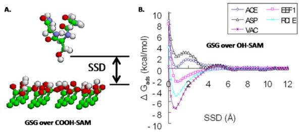
(a) Molecular model of a peptide a with sequence of GSG (glycine-serine-glycine) over a functionalized SAM surface. SSD (surface separation distance) represents the separation distance between the side group of the middle residue of the peptide and the top layer of the surface. (b) Plot showing calculated values of adsorption free energy vs SSD for a GSG peptide over a hydrophilic OH-SAM surface used for four different implicit solvation methods and vacuum (Ref. 105). As shown, each implicit model provides a very different prediction of the adsorption behavior for this peptide-surface combination. Adapted from Ref. 105; used with permission.

VI. Sampling

The third critical issue that must be addressed in any molecular simulation is the issue of sampling. Discussion of this issue will primarily be restricted to MD simulations, although sampling problems are equally of concern when using MC methods. To appreciate the importance of this, it must be realized that a conventional MD simulation typically represents the behavior of a single molecule over a simulated time scale of tens of nanoseconds, while an experimental measurement represents an ensemble average of the behavior of billions of molecules over time spans of milliseconds and longer. This situation raises the obvious question of how can the results of a MD simulation possibly be compared to an experimental measurement? The answer to this question is that MD simulation results can indeed be compared to experimental results if the simulated system is appropriately represented and sufficiently sampled. One of the main problems with this, however, is that it is often difficult to achieve the necessary degree of sampling.

As a complicating factor related to this problem, systems involving the behavior of complex molecular structures, such as a peptide or a protein adsorbing on a surface, generally exhibit a very rough potential energy surface, which represents the relationship between the potential energy as a function of the coordinates of the system, also referred to as the configurational phase space. This potential energy surface typically has numerous local low-energy positions that are separated from one another by relatively high potential energy barriers (e.g., barriers separating trans and gauche states for dihedral bond rotation). Because of this situation, a conventional MD simulation of the system will often become trapped in one or only a few of the many local low-energy wells, or even in the global low-energy well, for the entire simulation, thus providing a very poor representation of the correct ensemble-average behavior of the molecular system. An illustration of this problem is provided in Fig. 3, which shows simulation results for two different peptide-surface systems; one that did not exhibit a strong adsorption response and the other that did. The strongly adsorbing system encountered a substantial sampling problem that prevented the calculation of adsorption free energy from the simulation results for that system.

Fig. 3.

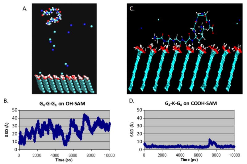
(a) A snapshot from the trajectory file of a G₄-G-G₄ peptide over an OH-SAM surface during a 10 ns MD simulation. The small single spheres are sodium and chloride ions in solution. (b) SSD between the peptide and the SAM surface for the molecular system shown in (a) vs simulated time showing that the peptide was able to sample over the entire SSD-coordinate space without being trapped in any one position. This occurred in this case because the peptide did not strongly adsorb to the surface. (c) A snapshot from the trajectory file of a G₄-K-G₄ peptide over a COOH-SAM surface. In this case, the peptide adsorbed tightly to the surface. (d) SSD vs simulated time for the peptide-SAM system shown in (c). A severe sampling problem is shown in that the peptide does not escape from the surface during the whole simulation, thus providing insufficient sampling for the proper calculation of adsorption free energy from the simulation results. Adapted from Ref. 76; used with permission.

To overcome this type of problem, advanced sampling methods can be employed that introduce an artificial driving force into the simulation that enables the system to escape from designated low-energy positions and more fully explore the entire phase space of the system. Following the simulation, the effects of this artificially applied forcing function can be removed to provide a proper unbiased set of sampled states, which can then be used to calculate correct ensemble-average properties of system behavior that can be compared to experimental measurements. As addressed below, several different types of methods have been developed to deal with different types of sampling problems, and it is important to select the method, or combination of methods, that will address the particular sampling problems that are being encountered for a given molecular system.

To understand advanced sampling methods, it is necessary to first understand a few of the basic relationships of statistical mechanics that determine the probability of sampling a given state of a molecular system during a molecular simulation and how this is related to the potential energy and the changes in free energy of the system. The probability of a given energy state being sampled (P_i) and the relative probability of sampling a different energy state P_j relative to P_i (i.e., P_j/P_i) can be expressed as¹⁰⁷

$$P_i=\frac{{\Omega }_i{e}^{-E_i/k_{B}T}}{Q},$$

with

$$Q=\sum _i{\Omega }_i{e}^{-E_i/k_{B}T}$$ (2)

and

$$P_{ij}\equiv \frac{P_j}{P_i}=\frac{{\Omega }_j}{{\Omega }_i}{e}^{-\Delta E_{ij}/k_{B}T}=e^{-\Delta G_{ij}/k_{B}T},$$ (3)

respectively, where E_i is the potential energy of the system for energy state i, Ω_i is the degeneracy of the system for energy state E_i (i.e., the number of different ways that the atoms in the system can be configured to have an overall system potential energy of E_i), k_B is the Boltzmann constant, T is absolute temperature, Q is the configurational partition function of the system, ΔE_ij is the difference in potential energy between states i and j, and ΔG_ij is the difference in free energy for the system between states i and j. Given these relationships, the probability of the system being in a given energy state can be adjusted by altering the value of the group of parameters in the exponential (i.e., E_i/k_BT), either by introducing a biasing-energy function into the force field equation to influence the energy state of the system (E_i) or by adjusting the temperature of the system (T).

Accordingly, if the molecular system is trapped in a given local low-energy minimum position with energy state E_i, a biasing-energy function (ΔB_ij) can be added to the force field equation to counter the effect of the local low-energy well, as shown in Eq. (4),

$${\overline{P}}_{ij}\equiv \frac{P_j}{P_i}{e}^{-\Delta B_{ij}/k_{B}T}=\frac{{\Omega }_j}{{\Omega }_i}{e}^{-(\Delta E_{ij}+\Delta B_{ij})/k_{B}T}=e^{-(\Delta G_{ij}+\Delta B_{ij})/k_{B}T}.$$ (4)

If adequately applied, this effectively “fills” the energy well to prevent the molecular system from being trapped in that region of coordinate space. This, of course, results in a biased-probability distribution P̄_ij being sampled during the simulation. As shown in Eq. (5),

$$P_{ij}\equiv \frac{P_j}{P_i}={\overline{P}}_{ij}{e}^{\Delta B_{ij}/k_{B}T},\Delta G_{ij}=-kTln({\overline{P}}_{ij})-\Delta B_{ij},$$ (5)

this biased-probability distribution can then be corrected following the simulation to obtain the unbiased-probability distribution P_ij, from which the difference in free energy between states i and j can be calculated. This method is highly effective if the coordinate position and the depth of a given local low-energy well are known such that a biasing-energy function can be appropriately determined and applied in the simulation. If these factors are not known a priori, they can be determined by running preliminary MD simulations to assess where the system tends to become trapped, and then adaptively adding in a biasing function until the sampling problem is overcome.^108–111

The use of a biased-energy function is most widely used to control sampling over a single designated system coordinate, such as the dihedral rotation about a bond in a peptide chain¹¹² or the separation distance between a peptide and a surface.⁸¹ For these types of applications, an umbrella sampling technique^108,113 is typically used in the form of

$$\Delta B=k_u{(\theta -{\theta }_h)}^2,$$ (6)

which is also referred to as a restraining potential, where k_u is the force constant, θ_h is the coordinate parameter of interest, which is set at a designated coordinate value, and θ is the sampled value of the coordinate at a given point in the simulation. In this form, the biasing-energy function penalizes the system in a quadratically increasing manner as it deviates from the designated position θ_h. A series of independent parallel simulations, referred to as windows, can then be carried out with the value of θ_h incrementally varied over the full range of interest, with these increments set such that the neighboring sampled populations overlap one another. The results of all of these simulations can then be combined using the weighted histogram analysis method,^114–116 which serves to correct the sampling distribution for the applied bias and generate an unbiased-probability distribution of states over the full range of the parameter of interest (i.e., θ). This unbiased-probability distribution can then be used to calculate the potential of mean force (PMF) of the system, which is equivalent to free energy, as a function of the change of the designated coordinate (θ). While this method is very useful for many different situations, it has the distinct drawback of becoming extremely complicated when applied to more than one parameter at a time.

As an alternative to the use of biased-energy functions, sampling of a system can also be greatly enhanced by raising the temperature of the simulation. In this case, the increased temperature level provides additional thermal energy in the simulation, which then also has the effect of enabling the system to more rapidly escape from local energy minima. The distinct advantage of the use of temperature in this manner is that it influences all of the degrees of freedom of the system at the same time, thus facilitating the crossing of all energy barriers in the system during a simulation without requiring knowledge of their location.

One of the most widely used and well-developed methods to accomplish this type of sampling is known as replica exchange molecular dynamics (REMD),^117,118 which is based on a previously developed method called parallel tempering.¹¹⁹ With this method, independent MD simulations are run for a series of replicas of a given molecular system with each replica being run at an increasingly higher temperature level above a baseline temperature of interest, e.g., 298 K. After a short user-designated time period (e.g., 250 steps of MD), a statistical mechanics–based exchange algorithm similar to that used in a Metropolis Monte Carlo exchange process¹²⁰ is used to compare the potential energy levels between replicas at neighboring temperatures. If the exchange is accepted, then the temperature levels between the pair of replicas are swapped. If it is not, the replicas remain at their prior temperature levels for another sampling cycle, following which the swapping decision process is repeated again. A diagram depicting this process is shown in Fig. 4. By this method, a replica that is trapped in a local low-energy well that actually represents a relative high energy level of the system tends to be exchanged upward in temperature. This then provides additional thermal energy to help that replica escape from the energy well to potentially explore other more favorable states of the system. Similarly, replicas that happen to be close to the global low-energy position tend to be exchanged downward in temperature, thus increasing their probability of ending up being sampled at the baseline temperature. The effect of this somewhat complicated process is to greatly enhance the sampling of the coordinate phase space of a molecular system and, in the end, generate a Boltzmann-weighted ensemble of states at each temperature level. The value of this is that the resulting sampled distribution of states then represents an equilibrated system of states that effectively transcends the time domain, thus enabling ensemble-averaged properties of the system to be determined from this distribution that theoretically should be comparable to experimental measurements of a similar system under equilibrium conditions. While this is an extremely useful computational technique, it can require that a very large number of replicas be used in order to span the range of temperature that is necessary to enhance energy-barrier crossing, and it still requires that a very large amount of sampling be conducted to obtain a properly converged ensemble of states at the baseline temperature of interest. The combination of these two requirements thus means that a very large amount of computing resources is often needed for the use of this method. To address these types of limitations, many different versions of this method have been and are being developed to improve computational efficiency,^121–125 including methods that vary the potential energy function instead of temperature.^126,127

Fig. 4.

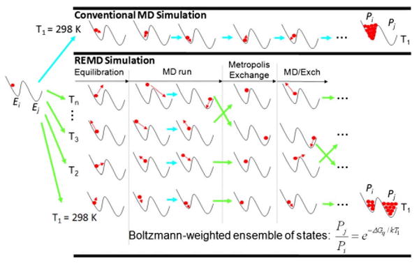
Schematic comparison of a conventional MD simulation compared to an REMD simulation for a simple model system containing two potential energy wells separated by an energy barrier. The MD simulation is not able to get over the energy barrier separating the two local low-energy wells and thus is shown to be trapped in the single local low-energy well during the entire simulation, resulting in a poorly sampled system. The REMD simulation uses thermal energy to enable the system to readily cross the energy barrier. The Metropolis-type exchange procedure used to swap temperature levels enables the development of a Boltzmann-weighted ensemble of states being sampled at the baseline temperature, thus representing a properly sampled, equilibrated system with ensemble-average properties that should be comparable to experimental measurements.

The type of advanced sampling algorithm that should be used for a given simulation will depend on the type of sampling problems that must be dealt with in a given molecular system. For example, to effectively and efficiently sample the behavior of peptide-surface interactions for the calculation of adsorption free energy using a designated force field, we have actually found that we must combine both biased-energy and REMD methods in order to perform a biased-energy REMD simulation.⁸¹ This is needed because this type of molecular system actually has two different types of sampling problems that need to be overcome. The first is that for a strongly adsorbing peptide-surface combination, the peptide will tend to become trapped against the surface,^77,128 thus failing to explore the configurational space far removed from the surface. This type of sampling problem can be readily addressed using windowed umbrella sampling, but not by REMD.⁸¹ The second sampling problem is the need to adequately sample the configurational space of the peptide in solution, with each dihedral angle of the peptide tending to be trapped in its own local low-energy state during a simulation. In this case, there are simply too many different coordinates that need to be controlled, thus greatly complicating the use of umbrella sampling methods to address this issue. REMD methods, on the other hand, are very well suited for this type of sampling problem by providing elevated temperature conditions to facilitate dihedral rotation about each of the rotatable covalent bonds of the peptide.

To set up for this type of simulation, a PMF profile over the coordinate representing the distance between the peptide and the surface, or the surface separation distance (SSD), is first determined from a series of MD simulations at a desired baseline temperature (e.g., 298 or 310 K) using windowed umbrella sampling over the SSD coordinate. A biased-energy function is then defined as the negative of the PMF versus SSD profile; which, when incorporated into a MD simulation, should effectively cancel the attraction of the surface for the peptide, thus enabling the peptide to randomly move up and down over the surface during the simulation. This biasing-energy function is then added to the force field equation and a REMD simulation is conducted to provide a biased-REMD simulation that is capable of overcoming both types of sampling problems (i.e., dihedral rotation and SSD trapping) at once. After the simulation is completed, the sampled biased-probability distribution is corrected for the applied biasing function. The results from this type of simulation then provide an equilibrated ensemble of states with a probability distribution that properly reflects the strength of interaction between the peptide and the surface.⁸¹ This probability distribution can thus be used to calculate the adsorption free energy for comparison with experimental data.⁸⁰ These types of simulations⁸¹ and experiments⁸⁰ are currently being conducted with the CHARMM force field so that the accuracy of this force field can be assessed and its parameters can be corrected as necessary for the development of a validated interfacial force field for use for the simulation of peptide-surface and protein-surface interactions.

VII. Future Directions

New methods and algorithms in the computational chemistry field are continually being developed and refined to improve the capabilities of molecular simulation. For example, new capabilities are being pioneered for the extension of quantum mechanical methods for MD simulations.^129–131 Others are working on the development of combined quantum mechanics/molecular mechanics (QM/MM) methods in which quantum mechanics calculations are used to model small groups of atoms of particular interest within a larger molecular framework that is treated with an all-atom empirical force field.^132–134 Other areas of development include efforts to develop polarizable empirical force fields with force field parametrization that is able to adapt to its local surroundings,^70–74 and empirical force fields that provide for bond breaking/forming capabilities,^47–49 both of which enable quantum mechanical effects to be included in an empirical force field for MM, MC, and MD simulations.

While all of these areas will likely lead to advancements in the capabilities for performing accurate molecular simulations, the most promising areas of new development that will most directly impact the ability to predict protein-surface interactions are the development of multiscale modeling methods.^135–137 These methods seek to develop and apply coarse-graining techniques that will enable time and length scales to be spanned to link all-atom representations of a system at the nanosecond time scale all the way to continuum macroscopic-level representations of a system for processes occurring over time frames of seconds and longer.

VIII. Concluding Remarks

Molecular simulation is a rapidly developing field. Not only is computational power continuing to advance but algorithm development to further improve the way that computational resources are used also continues to progress at a rapid pace. Thus while current computational resources may be insufficient at this time to enable simulations to be conducted to predict the competitive adsorption behavior of large proteins on biomaterials surfaces to form an equilibrated adsorbed protein layer, and to predict the interactions of membrane-bound cell receptors with this adsorbed protein layer, it is highly likely that within a decade or two that these types of systems will be able to be readily handled. These prospects, coupled with the rapidly developing field of nanotechnology, hold promise for the eventual development of the capabilities of actually being able to proactively design surfaces at the atomic level to specifically control the manner that proteins adsorb, thus controlling surface bioactivity and subsequent cellular response for a broad range of applications in biotechnology and biomedical engineering.

Before these capabilities can be achieved, however, accurate molecular simulation methods must first be developed, including the development of validated force fields for protein-surface interactions, methods to accurately represent solvation effects, advanced sampling algorithms for the efficient prediction of equilibrated ensemble-averaged properties, and multiscale modeling techniques to extend time and length scales. By working out solutions to these types of problems now, methods will be in place by the time computational power advances to the point of using this technology as a powerful tool to finally achieve the long-term goal of being able to predict and control protein-surface interactions.

References

- 1.Castner DG, Ratner BD. Surf Sci. 2002;500:28. [Google Scholar]
- 2.Hlady V, Buijs J. Curr Opin Biotechnol. 1996;7:72. doi: 10.1016/s0958-1669(96)80098-x. [DOI] [PMC free article] [PubMed] [Google Scholar]
- 3.Tsai WB, Grunkemeier JM, McFarland CD, Horbett TA. J Biomed Mater Res. 2002;60:348. doi: 10.1002/jbm.10048. [DOI] [PubMed] [Google Scholar]
- 4.Latour RA. The Encyclopedia of Biomaterials and Bioengineering. Taylor & Francis; New York: 2005. pp. 1–15. [Google Scholar]
- 5.Dee KC, Puleo DA, Bizios R. Tissue-Biomaterials Interactions. Wiley; Hoboken, NJ: 2002. pp. 45–49. [Google Scholar]
- 6.Geelhood SJ, Horbett TA, Ward WK, Wood MD, Quinn MJ. J Biomed Mater Res, Part B: Appl Biomater. 2007;81B:251. doi: 10.1002/jbm.b.30660. [DOI] [PubMed] [Google Scholar]
- 7.Lange K, Grimm S, Rapp M. Sens Actuators B. 2007;125:441. [Google Scholar]
- 8.Aubin-Tam ME, Zhou H, Hamad-Schifferli K. Soft Mater. 2008;4:554. doi: 10.1039/b711937b. [DOI] [PubMed] [Google Scholar]
- 9.Hall JB, Dobrovolskaia MA, Patri AK, McNeil SE. Nanomedicine. 2007;2:789. doi: 10.2217/17435889.2.6.789. [DOI] [PubMed] [Google Scholar]
- 10.Hung CW, Holoman TRP, Kofinas P, Bentley WE. Biochem Eng J. 2008;38:164. [Google Scholar]
- 11.Lynch I, Dawson KA. Nanotoday. 2008;3:40. [Google Scholar]
- 12.Mu QX, et al. J Phys Chem C. 2008;112:3300. [Google Scholar]
- 13.Hartmann M. Chem Mater. 2005;17:4577. [Google Scholar]
- 14.Shüler C, Carusa F. Macromol Rapid Commun. 2000;21:750. [Google Scholar]
- 15.Yang HH, Zhang SQ, Chen XL, Zhuang ZX, Xu JG, Wang XR. Anal Chem. 2004;76:1316. doi: 10.1021/ac034920m. [DOI] [PubMed] [Google Scholar]
- 16.Yu AM, Liang ZJ, Caruso F. Chem Mater. 2005;17:171. [Google Scholar]
- 17.Kusnezow W, Hoheisel JD. BioTechniques Suppl S. 2002:14. [PubMed] [Google Scholar]
- 18.Steinhauer C, Wingren C, Hager AC, Borrebaeck CA. BioTechniques Suppl S. 2002:38. [PubMed] [Google Scholar]
- 19.Shankaran DRM, Miura N. J Phys D. 2007;40:7187. [Google Scholar]
- 20.Salmain M, Fischer-Durand N, Pradier CM. Anal Biochem. 2008;373:61. doi: 10.1016/j.ab.2007.10.031. [DOI] [PubMed] [Google Scholar]
- 21.Sanchez S, Pumera M, Fabregas E. Biosens Bioelectron. 2007;23:332. doi: 10.1016/j.bios.2007.04.021. [DOI] [PubMed] [Google Scholar]
- 22.Wang HX, Meng S, Guo K, Liu Y, Yang PY, Zhong W, Liu BH. Electrochem Commun. 2008;10:447. [Google Scholar]
- 23.Goto Y, Matsuno R, Konno T, Takai M, Ishihara K. Biomacromolecules. 2008;9:828. doi: 10.1021/bm701161d. [DOI] [PubMed] [Google Scholar]
- 24.Beck DAC, Daggett V. Methods. 2004;34:112. doi: 10.1016/j.ymeth.2004.03.008. [DOI] [PubMed] [Google Scholar]
- 25.Brooks CL., III Curr Opin Struct Biol. 1998;8:222. doi: 10.1016/s0959-440x(98)80043-2. [DOI] [PubMed] [Google Scholar]
- 26.Ferrara P, Apostolakis J, Caflisch A. J Phys Chem B. 2000;104:5000. [Google Scholar]
- 27.Fersht AR, Daggett V. Cell. 2002;108:573. doi: 10.1016/s0092-8674(02)00620-7. [DOI] [PubMed] [Google Scholar]
- 28.Gnanakaran S, Nymeyer H, Portman J, Sanbonmatsu KY, Garcia AE. Curr Opin Struct Biol. 2003;13:168. doi: 10.1016/s0959-440x(03)00040-x. [DOI] [PubMed] [Google Scholar]
- 29.Hofinger S, Almeida B, Hansmann UHE. Proteins. 2007;68:662. doi: 10.1002/prot.21268. [DOI] [PubMed] [Google Scholar]
- 30.Jang SM, Kim E, Pak YS. J Chem Phys. 2008;128:105102. doi: 10.1063/1.2837655. [DOI] [PubMed] [Google Scholar]
- 31.Schaeffer RD, Fersht A, Daggett V. Curr Opin Struct Biol. 2008;18:4. doi: 10.1016/j.sbi.2007.11.007. [DOI] [PMC free article] [PubMed] [Google Scholar]
- 32.Wang W, Donini O, Reyes CM, Kollman PA. Annu Rev Biophys Biomol Struct. 2001;30:211. doi: 10.1146/annurev.biophys.30.1.211. [DOI] [PubMed] [Google Scholar]
- 33.Halperin I, Ma BY, Wolfson H, Nussinov R. Proteins. 2002;47:409. doi: 10.1002/prot.10115. [DOI] [PubMed] [Google Scholar]
- 34.Ehrlich LP, Nilges M, Wade RC. Proteins. 2005;58:126. doi: 10.1002/prot.20272. [DOI] [PubMed] [Google Scholar]
- 35.De Grandis V, Bizzarri AR, Cannistraro S. J Mol Recognit. 2007;20:215. doi: 10.1002/jmr.840. [DOI] [PubMed] [Google Scholar]
- 36.Costantini S, Colonna G, Facchiano AM. Comput Biol Chem. 2007;31:196. doi: 10.1016/j.compbiolchem.2007.03.010. [DOI] [PubMed] [Google Scholar]
- 37.Chandrasekaran V, Ambati J, Ambati BK, Taylor EW. J Mol Graphics Modell. 2007;26:775. doi: 10.1016/j.jmgm.2007.05.001. [DOI] [PubMed] [Google Scholar]
- 38.Bond PJ, Sansom MSP. J Am Chem Soc. 2006;128:2697. doi: 10.1021/ja0569104. [DOI] [PMC free article] [PubMed] [Google Scholar]
- 39.Efremov RG, Nolde DE, Vergoten G, Arseniev AS. Biophys J. 1999;76:2460. doi: 10.1016/S0006-3495(99)77401-1. [DOI] [PMC free article] [PubMed] [Google Scholar]
- 40.Hyvonen MT, Oorni K, Kovanen PT, Ala-Korpela M. Biophys J. 2001;80:565. doi: 10.1016/S0006-3495(01)76038-9. [DOI] [PMC free article] [PubMed] [Google Scholar]
- 41.Muegge I. Med Res Rev. 2003;23:302. doi: 10.1002/med.10041. [DOI] [PubMed] [Google Scholar]
- 42.Bernard D, Coop A, Mackerell AD. J Med Chem. 2005;48:7773. doi: 10.1021/jm050785p. [DOI] [PubMed] [Google Scholar]
- 43.Chen HF. Chem Biol Drug Des. 2008;71:434. doi: 10.1111/j.1747-0285.2008.00656.x. [DOI] [PubMed] [Google Scholar]
- 44.Fischer B, Fukuzawa K, Wenzel W. Proteins. 2008;70:1264. doi: 10.1002/prot.21607. [DOI] [PubMed] [Google Scholar]
- 45.Waszkowycz B. Drug Discovery Today. 2008;13:219. doi: 10.1016/j.drudis.2007.12.002. [DOI] [PubMed] [Google Scholar]
- 46.Leach AR. Molecular Modelling: Principles and Applications. Pearson Education; Harlow, UK: 1996. pp. 131–206. [Google Scholar]
- 47.Brenner DW, Shenderova OA, Harrison JA, Stuart SJ, Ni B, Sinnott SB. J Phys: Condens Matter. 2002;14:783. [Google Scholar]
- 48.Ni B, Lee KH, Sinnott SB. J Phys: Condens Matter. 2004;16:7261. [Google Scholar]
- 49.Liu A, Stuart SJ. J Comput Chem. 2008;29:601. doi: 10.1002/jcc.20817. [DOI] [PubMed] [Google Scholar]
- 50.Weiner SJ, Kollman PA, Case DA, Singh UC, Ghio C, Alagona G, Profeta JS, Weiner P. J Am Chem Soc. 1984;106:765. [Google Scholar]
- 51.Cornell WD, et al. J Am Chem Soc. 1995;117:5179. [Google Scholar]
- 52.Brooks BR, Bruccoleri RE, Olafson BD, States DJ, Swaminathan S, Karplus M. J Comput Chem. 1983;4:187. [Google Scholar]
- 53.MacKerell ADJ, Brooks B, Brooks CLI, Nilsson L, Roux B, Won Y, Karplus M. Encyclopedia of Computational Chemistry. Wiley; New York: 1998. pp. 271–277. [Google Scholar]
- 54.Jorgensen WL, Tirado-Rives J. J Am Chem Soc. 1988;110:1657. doi: 10.1021/ja00214a001. [DOI] [PubMed] [Google Scholar]
- 55.Kaminski GA, Friesner RA, Tirado-Rives J, Jorgensen WL. J Phys Chem B. 2001;105:6474. [Google Scholar]
- 56.van Gunsteren WF, Daura X, Mark AE. Encyclopedia of Compuational Chemistry. Vol. 2. Wiley; New York: 1998. pp. 1211–1216. [Google Scholar]
- 57.Scott WRP, et al. J Phys Chem A. 1999;103:3596. [Google Scholar]
- 58.Allinger NL. J Am Chem Soc. 1977;99:8127. [Google Scholar]
- 59.Allinger NL, Yuh YH, Lii JH. J Am Chem Soc. 1989;111:8551. [Google Scholar]
- 60.Allinger NL, Chen K, Lii LH. J Comput Chem. 1996;17:642. [Google Scholar]
- 61.Hwang MJ, Stockfisch TP, Hagler AT. J Am Chem Soc. 1994;116:2515. [Google Scholar]
- 62.Soldera A. Polymer. 2002;43:4269. [Google Scholar]
- 63.Blomqvist J. Polymer. 2001;42:3515. [Google Scholar]
- 64.Lee S, Jeong HY, Lee H. Comput Theor Polym Sci. 2001;11:219. [Google Scholar]
- 65.Bunte SW, Sun H. J Phys Chem B. 2000;104:2477. [Google Scholar]
- 66.McQuaid MJ, Sun H, Rigby D. J Comput Chem. 2004;25:61. doi: 10.1002/jcc.10316. [DOI] [PubMed] [Google Scholar]
- 67.Sun H. J Phys Chem B. 1998;102:7338. [Google Scholar]
- 68.MacKerell AD. J Comput Chem. 2004;25:1584. doi: 10.1002/jcc.20082. [DOI] [PubMed] [Google Scholar]
- 69.Yin D, MacKerell AD., Jr J Comput Chem. 1998;19:334. [Google Scholar]
- 70.Rick SW, Stuart SJ. Reviews in Computational Chemistry. Wiley; New York: 2002. pp. 89–146. [Google Scholar]
- 71.Geerke DP, van Gunsteren WF. Mol Phys. 2007;105:1861. [Google Scholar]
- 72.Paesani F, Iuchi S, Voth GA. J Chem Phys. 2007;127:074506. doi: 10.1063/1.2759484. [DOI] [PubMed] [Google Scholar]
- 73.Warshel A, Kato M, Pisliakov AV. J Chem Theory Comput. 2007;3:2034. doi: 10.1021/ct700127w. [DOI] [PubMed] [Google Scholar]
- 74.Kaminski GA, Stern HA, Berne BJ, Friesner RA, Cao YXX, Murphy RB, Zhou RH, Halgren TA. J Comput Chem. 2002;23:1515. doi: 10.1002/jcc.10125. [DOI] [PMC free article] [PubMed] [Google Scholar]
- 75.Oostenbrink C, Villa A, Mark AE, van Gunsteren WF. J Comput Chem. 2004;25:1656. doi: 10.1002/jcc.20090. [DOI] [PubMed] [Google Scholar]
- 76.Raut VP, Agashe M, Stuart SJ, Latour RA. Langmuir. 2005;21:1629. doi: 10.1021/la047807f. [DOI] [PubMed] [Google Scholar]
- 77.Raut VP, Agashe MA, Stuart SJ, Latour RA. Langmuir. 2006;22:2402. doi: 10.1021/la047807f. [DOI] [PubMed] [Google Scholar]
- 78.Prime KL, Whitesides GM. J Am Chem Soc. 1993;115:10714. [Google Scholar]
- 79.Vernekar VN, Latour RA. Mater Res Innovations. 2005;9:337. [Google Scholar]
- 80.Wei Y, Latour RA. Langmuir. 2008;24:6721. doi: 10.1021/la8005772. [DOI] [PMC free article] [PubMed] [Google Scholar]
- 81.Wang F, Stuart SJ, Latour RA. BioInterphases. 2008;3:9. doi: 10.1116/1.2840054. [DOI] [PMC free article] [PubMed] [Google Scholar]
- 82.Glattli A, Daura X, van Gunsteren WF. J Chem Phys. 2002;116:9811. [Google Scholar]
- 83.Mark P, Nilsson L. J Phys Chem A. 2001;105:9954. [Google Scholar]
- 84.Jorgensen WL, Chandrasekhar J, Madura JD, Impey RW, Klein ML. J Chem Phys. 1983;79:926. [Google Scholar]
- 85.Jorgensen WL, Madura JD. Mol Phys. 1985;56:1381. [Google Scholar]
- 86.Jorgensen WL, Jenson C. J Comput Chem. 1998;19:1179. [Google Scholar]
- 87.Horn HW, Swope WC, Pitera JW, Madura JD, Dick TJ, Hura GL, Head-Gordon T. J Chem Phys. 2004;120:9665. doi: 10.1063/1.1683075. [DOI] [PubMed] [Google Scholar]
- 88.Horn HW, Swope WC, Pitera JW. J Chem Phys. 2005;123:194504. doi: 10.1063/1.2085031. [DOI] [PubMed] [Google Scholar]
- 89.Mahoney MW, Jorgensen WL. J Chem Phys. 2001;114:363. [Google Scholar]
- 90.Rick SW, Stuart SJ, Bader JS, Berne BJ. J Mol Liq. 1995;65–66:31. [Google Scholar]
- 91.Garemyr R, Elofsson A. Proteins. 1999;37:417. doi: 10.1002/(sici)1097-0134(19991115)37:3<417::aid-prot9>3.0.co;2-u. [DOI] [PubMed] [Google Scholar]
- 92.CRC. Handbook of Chemistry and Physic. 67. CRC; Boca Rotan, FL: 1986–1987. p. E-56. [Google Scholar]
- 93.Israelachvili J. Intermolecular and Surface Forces. Academic; San Diego, CA: 1992. p. 41. [Google Scholar]
- 94.Schaefer M, Bartels C, Karplus M. Theor Chem Acc. 1999;101:194. [Google Scholar]
- 95.Sharp KA, Honig B. J Phys Chem. 1990;94:7684. [Google Scholar]
- 96.Bertonati C, Honig B, Alexov E. Biophys J. 2007;92:1891. doi: 10.1529/biophysj.106.092122. [DOI] [PMC free article] [PubMed] [Google Scholar]
- 97.Still WC, Tempczyk A, Hawley RC, Hendrickson T. J Am Chem Soc. 1990;112:6127. [Google Scholar]
- 98.Dominy BN, Brooks CL., III J Phys Chem B. 1999;103:3765. [Google Scholar]
- 99.Bashford D, Case DA. Annu Rev Phys Chem. 2000;51:129. doi: 10.1146/annurev.physchem.51.1.129. [DOI] [PubMed] [Google Scholar]
- 100.Feig M, Brooks CL., III Curr Opin Struct Biol. 2004;14:217. doi: 10.1016/j.sbi.2004.03.009. [DOI] [PubMed] [Google Scholar]
- 101.Feig M, Onufriev A, Lee MS, Im W, Case DA, Brooks CL. J Comput Chem. 2004;25:265. doi: 10.1002/jcc.10378. [DOI] [PubMed] [Google Scholar]
- 102.Zhou R, Berne BJ. Proc Natl Acad Sci USA. 2002;99:12777. doi: 10.1073/pnas.142430099. [DOI] [PMC free article] [PubMed] [Google Scholar]
- 103.Sitkoff D, Sharp KA, Honig B. J Phys Chem. 1994;98:1978. [Google Scholar]
- 104.Qiu D, Shenkin PS, Hollinger FP, Still WC. J Phys Chem A. 1997;101:3005. [Google Scholar]
- 105.Sun Y, Latour RA. J Comput Chem. 2006;27:1908. doi: 10.1002/jcc.20488. [DOI] [PubMed] [Google Scholar]
- 106.Sun Y, Dominy BN, Latour RA. J Comput Chem. 2007;28:1883. doi: 10.1002/jcc.20716. [DOI] [PubMed] [Google Scholar]
- 107.McQuarrie DA. Statistical Thermodynamics. University Science Books; Mill Valley, CA: 1973. pp. 35–47. [Google Scholar]
- 108.Harvey SC, Prabhakaran M. J Phys Chem. 1987;91:4799. [Google Scholar]
- 109.Roux B. Comput Phys Commun. 1995;91:275. [Google Scholar]
- 110.Mezei M. J Comput Phys. 1987;68:237. [Google Scholar]
- 111.Bartels C, Karplus M. J Phys Chem B. 1998;102:865. [Google Scholar]
- 112.Bartels C, Karplus M. J Comput Chem. 1997;18:1450. doi: 10.1002/jcc.1137. [DOI] [PubMed] [Google Scholar]
- 113.Beutler TC, Vangunsteren WF. J Chem Phys. 1994;100:1492. [Google Scholar]
- 114.Kumar S, Bouzida D, Swendsen RH, Kollman PA, Rosenberg JM. J Comput Chem. 1992;13:1011. [Google Scholar]
- 115.Kumar S, Rosenberg JM, Bouzida D, Swendsen RH, Kollman PA. J Comput Chem. 1995;16:1339. [Google Scholar]
- 116.Gallicchio E, Andrec M, Felts AK, Levy RM. J Phys Chem B. 2005;109:6722. doi: 10.1021/jp045294f. [DOI] [PubMed] [Google Scholar]
- 117.Sugita Y, Okamoto Y. Chem Phys Lett. 1999;314:141. [Google Scholar]
- 118.Garcia AE, Sanbonmatsu KY. Proteins. 2001;42:345. doi: 10.1002/1097-0134(20010215)42:3<345::aid-prot50>3.0.co;2-h. [DOI] [PubMed] [Google Scholar]
- 119.Hansmann UHE. Chem Phys Lett. 1997;281:140. [Google Scholar]
- 120.Leach AR. Molecular Modelling: Principles and Applications. Pearson Education; Harlow, UK: 1996. pp. 407–408. [Google Scholar]
- 121.Mitsutake A, Sugita Y, Okamoto Y. Biopolymers. 2001;60:96. doi: 10.1002/1097-0282(2001)60:2<96::AID-BIP1007>3.0.CO;2-F. [DOI] [PubMed] [Google Scholar]
- 122.Okamoto Y. J Mol Graphics Modell. 2004;22:425. doi: 10.1016/j.jmgm.2003.12.009. [DOI] [PubMed] [Google Scholar]
- 123.Okur A, Wickstrom L, Layten M, Geney R, Song K, Hornak V, Simmerling C. J Chem Theory Comput. 2006;2:420. doi: 10.1021/ct050196z. [DOI] [PubMed] [Google Scholar]
- 124.Okur A, Roe DR, Cui GL, Hornak V, Simmerling C. J Chem Theory Comput. 2007;3:557. doi: 10.1021/ct600263e. [DOI] [PubMed] [Google Scholar]
- 125.Li XF, O'Brien CP, Collier G, Vellore NA, Wang F, Latour RA, Bruce DA, Stuart SJ. J Chem Phys. 2007;127:164116. doi: 10.1063/1.2780152. [DOI] [PubMed] [Google Scholar]
- 126.Fukunishi H, Watanabe O, Takada S. J Chem Phys. 2002;116:9058. [Google Scholar]
- 127.Affentranger R, Tavernelli I, Di Iorio EE. J Chem Theory Comput. 2006;2:217. doi: 10.1021/ct050250b. [DOI] [PubMed] [Google Scholar]
- 128.Raut VP, Agashe MA, Stuart SJ, Latour RA. Langmuir. 2005;21:1629. doi: 10.1021/la047807f. [DOI] [PubMed] [Google Scholar]
- 129.Ludwig J, Vlachos DG. J Chem Phys. 2007;127:154716. doi: 10.1063/1.2794338. [DOI] [PubMed] [Google Scholar]
- 130.Ramondo F, Bencivenni L, Caminiti R, Pieretti A, Gontrani L. Phys Chem Chem Phys. 2007;9:2206. doi: 10.1039/b617837e. [DOI] [PubMed] [Google Scholar]
- 131.Li JL, Car R, Tang C, Wingreen NS. Proc Natl Acad Sci USA. 2007;104:2626. doi: 10.1073/pnas.0610945104. [DOI] [PMC free article] [PubMed] [Google Scholar]
- 132.Matsuura A, Sato H, Houjou H, Saito S, Hayashi T, Sakurai M. J Comput Chem. 2006;27:1623. doi: 10.1002/jcc.20432. [DOI] [PubMed] [Google Scholar]
- 133.Berges J, Rickards G, Rauk A, Houee-Levin C. Chem Phys Lett. 2006;421:63. [Google Scholar]
- 134.Riccardi D, Schaefer P, Cui Q. J Phys Chem B. 2005;109:17715. doi: 10.1021/jp0517192. [DOI] [PubMed] [Google Scholar]
- 135.Chu JW, Izveko S, Voth GA. Mol Simul. 2006;32:211. [Google Scholar]
- 136.de Pablo JJ, Curtin WA. MRS Bull. 2007;32:905. [Google Scholar]
- 137.Zhou J, Thorpe IF, Izvekov S, Voth GA. Biophys J. 2007;92:4289. doi: 10.1529/biophysj.106.094425. [DOI] [PMC free article] [PubMed] [Google Scholar]
- 138.Berendsen HJC, Vanderspoel D, Vandrunen R. Comput Phys Commun. 1995;91:43. [Google Scholar]