Restoration of DWI Data Using a Rician LMMSE Estimator

Abstract

This paper introduces and analyzes a linear minimum mean square error (LMMSE) estimator using a Rician noise model and its recursive version (RLMMSE) for the restoration of diffusion weighted images. A method to estimate the noise level based on local estimations of mean or variance is used to automatically parametrize the estimator. The restoration performance is evaluated using quality indexes and compared to alternative estimation schemes. The overall scheme is simple, robust, fast, and improves estimations. Filtering diffusion weighted magnetic resonance imaging (DW-MRI) with the proposed methodology leads to more accurate tensor estimations. Real and synthetic datasets are analyzed.

I. Introduction

DIFFUSION weighted magnetic resonance imaging (DW-MRI) allows for the measurement of water diffusivity. In particular, the directionality of water diffusion may be studied with appropriately selected gradient directions for diffusion measurements. Application areas for DW-MRI include neuroimaging studies [1] (where it can be used to determine the direction of white matter fibers and thus to determine brain connectivity), ischemic stroke detection [2], or the investigation of muscle fibers, e.g., within the heart [3], to name but a few.

Unlike structural MRI, where white matter appears as a region of uniform intensity, DW-MRI leads to diffusion direction dependent image intensities. In the case of anisotropic water diffusion, image intensities will be low if the measurement gradient direction is aligned with the major direction of diffusion and image intensities will be high for diffusion directions orthogonal to the measurement gradient direction.

Frequently, one aims at measuring the major diffusion direction as an indication of fiber orientation [4] and thus as a way to measure connectivity for example by tractography methods. Unfortunately, large diffusion causes low signal intensity, which results in a low signal-to-noise (SNR) ratio. If scanning time is not an issue, the SNR can be improved by repeated acquisitions and appropriate spatial averaging (assuming the subject does not move during the scan to avoid registration issues). However, high angular resolution DWI, where many gradient directions need to be acquired, may result in prohibitive scan durations for such physical averaging procedures. A postprocessing method to remove noise from DW images is thus desirable. Of note, besides noise influences, measurement data may for example be corrupted due to magnetic field inhomogeneities or subject motion. A comprehensive restoration methodology needs to account for such effects. This is beyond the scope of this paper, which focuses solely on the restoration of signals corrupted by measurement noise.

Various postprocessing methods to improve signal to noise ratios in MRI have been proposed.¹ One of the first attempts to estimate the magnitude MR image from a noisy image is due to Henkelman [5] who investigated the effect of noise on MR magnitude images, showed that the noise influence leads to an overestimation of the signal amplitude and provided a correction scheme based on image intensities. The conventional approach (CA) was proposed by McGibney et al. [6] utilizing the noise properties of the second image moment. Sijbers et al. [7]–[9] estimate the Rician noise level and perform signal reconstruction using a maximum likelihood (ML) approach. A similar method is used by Jiang and Yang [10]. Expectation maximization formulations with Rician noise assumptions have been used in synthetic aperture radar (SAR) imaging [11], [12]. Other approaches use wavelet-based methods for noise removal, as Nowak’s [13]—in which the authors assume an underlying Rician model—or the one due to Pižurica et al. [14]. McGraw et al. [15] use a weighted total-variation-norm denoising scheme, Ahn et al. [16] propose a template-based filtering procedure, and Martin-Fernandez et al. [17] propose an anisotropic Wiener-filter approach; all without using a Rician noise model. Basu et al. [18] use a Perona-Malik-like smoothing filter combined with a local Rician data attachment term (effectively trying to remove the intensity bias locally), assuming a known noise level for the Rician noise model. Recently, Koay and Basser [19] developed a correction scheme to analytically estimate the signal, also assuming the Rician model.

The method proposed in this paper is closest to the Wiener-filter approach by Martin-Fernandez et al. [17]. However, it assumes a Rician noise model and is paired with an automated method to estimate the Rician noise level.

Section II discusses the theory of the approach and gives some background on alternative estimation methods and Section III presents results. The conclusion is presented in Section IV.

II. Restoration of MR Data

A. Model of Noise in MRI

Noise in magnitude MRI images is usually modeled following a Rician distribution [7], [20], [21], due to the existence of uncorrelated Gaussian noise with zero mean and the same variance ${\sigma }_n^2$ in both the real and imaginary parts of the complex k-space data. Given the magnitude image M and the original signal amplitude A, the probability distribution function (PDF) of such an image is

$$p_M(M_{ij}\mid A_{ij},{\sigma }_n)=\frac{M_{ij}}{{\sigma }_n^2}{e}^{-\frac{M_{ij}^2+A_{ij}^2}{2{\sigma }_n^2}}{I}_0\left(\frac{A_{ij}{M}_{ij}}{{\sigma }_n^2}\right)u(M_{ij})$$ (1)

with I₀(·) being the 0th order modified Bessel function of the first kind, u(·) the Heaviside step function and ${\sigma }_n^2$ the variance of noise. M_ij is the magnitude value of the pixel (i, j) and A_ij the original value of the pixel without noise.

In the image background, where the SNR is low, the Rician PDF reduces to a Rayleigh distribution [22] with PDF

$$p_M(M_{ij}\mid {\sigma }_n)=p_M(M_{ij}\mid A_{ij}=0,{\sigma }_n)=\frac{M_{ij}}{{\sigma }_n^2}{e}^{-\frac{M_{ij}^2}{2{\sigma }_n^2}}u(M_{ij}).$$ (2)

Most signal estimation procedures rely on a given noise variance ${\sigma }_n^2$. Methods performing noise estimation from magnitude data may roughly be divided into two groups: 1) approaches estimating the noise variance using a single magnitude image and 2) approaches using multiple images. Noise estimation using a single image is usually based on background intensities (which need previous segmentation), where the true signal amplitude should vanish. Using the Rayleigh distribution, estimators based on the mean and the second order moment [23] can be defined as

$$\widehat{{\sigma }_n^2}=\frac{1}{2N}\sum _{i=1}^N{M}_i^2,\widehat{{\sigma }_n}=\sqrt{\frac{2}{\pi }}\frac{1}{N}\sum _{i=1}^N{M}_i$$ (3)

where N is the number of points considered for the estimation. Other estimators are based on the method of moments [10] and on the mode of the histogram [24].

B. Signal Estimation Methods

A number of techniques have been proposed to estimate the noise-free signal A from the noisy measurement signal M. Methods may be subdivided by the noise-model assumed. Basic filtering strategies include Gaussian smoothing and Wiener [25] filtering (also assuming a Gaussian noise model). More recently, estimators taking the Rician noise model into account have been developed. Since the approach proposed in this paper relates to this class of estimators, we briefly list and review some of the methods in what follows.

1. Conventional Approach (CA) [6]. Taking into account the relation between noise and signal of the second order moment in a Rician distribution, the signal can be estimated as

   $${\widehat{A}}_c=\sqrt{max(\langle M^2\rangle -2{\sigma }_n^2,0)}$$ (4)
   where 〈M²〉 is the sample second order moment. The sample estimator 〈.〉 is defined

   $$\langle I\rangle =\frac{1}{\mid \eta \mid }\sum _{p\in \eta }{I}_p$$ (5)

   with η a square neighborhood. This estimation may also be performed using nonsquare weighted windows, such as Gaussian functions.

2. ML estimator [7]–[10]. The signal is estimated by maximizing the likelihood function

   $${\widehat{A}}_{ML}=arg\underset{A}{max}(logL)$$ (6)
   with

   $$logL=\sum _{i=1}^{N}log\left(I_0\left(\frac{A{M}_i}{{\sigma }_n^2}\right)\right)-\frac{N{A}^2}{2{\sigma }_n^2}-\sum _{i=1}^N\frac{M_i^2}{2{\sigma }_n^2}$$ (7)

   where N is the number of samples considered for the likelihood function.

3. Expectation-maximization (EM) method [11], [12]. EM is a recursive method that aims at estimating the noise variance and the signal simultaneously trough maximization of the expected log likelihood

   $${\widehat{A}}_{k+1}=\frac{1}{N}\sum _{i=1}^N\frac{I_1\left(\frac{{\widehat{A}}_k{M}_i}{{\widehat{\sigma }}_k^2}\right)}{I_0\left(\frac{{\widehat{A}}_k{M}_i}{{\widehat{\sigma }}_k^2}\right)}{M}_i$$ (8)

   $${\widehat{\sigma }}_{k+1}^2=max\left[\frac{1}{2N}\sum _{i=1}^N{M}_i^2-\frac{{\widehat{A}}_k^2}{2},0\right].$$ (9)
   N is again the number of samples. The initial values are computed as

   $${\widehat{A}}_0={\left(2{\left(\frac{1}{N}\sum _{i=1}^N{M}_i^2\right)}^2-\frac{1}{N}\sum _{i=1}^N{M}_i^4\right)}^{1/4}$$ (10)

   $${\widehat{\sigma }}_0^2=\frac{1}{2}\left(\frac{1}{N}\sum _{i=1}^N{M}_i^2-{\widehat{A}}_0\right).$$ (11)
4. Analytically exact solution, proposed by Koay and Basser in [19]. Assuming a Rician noise model and given a measured sample mean 〈M〉 and a sample variance 〈M²〉 − 〈M〉², the signal and noise level are computed based on analytical relations. Given the correction factor

   $$\zeta (\theta )=2+{\theta }^2-\frac{\pi }{8}{e}^{-\frac{{\theta }^2}{2}}{\left[(2+{\theta }^2)I_0\left(\frac{{\theta }^2}{4}\right)+{\theta }^2{I}_1\left(\frac{{\theta }^2}{4}\right)\right]}^2$$
   and the root θ₀ of

   $$g(\theta ):=\sqrt{\zeta (\theta )\left(1+\frac{{\langle M\rangle }^2}{\langle M^2\rangle -{\langle M\rangle }^2}\right)-2}-\theta$$
   the signal estimation and the noise variance estimation may be computed as

   $$\begin{array}{l}{\widehat{\sigma }}^2=\frac{\langle M^2\rangle -{\langle M\rangle }^2}{\zeta ({\theta }_0)}\\ \widehat{A}={\theta }_0\widehat{\sigma }.\end{array}$$

   In all the cases, 〈.〉 is the sample estimator as defined in (5).

C. LMMSE Estimator for the Rician Model

The estimation method proposed in this paper (to estimate the signal from the noisy magnitude image) is based on the linear minimum mean square error (LMMSE) estimator. Instead of modeling the signal A_ij as an unknown constant, we consider it as a realization of a random variable which is functionally related to the observation. This way a closed-form analytical solution is achievable. This is in contrast to many other estimation techniques which find the solution via an iterative optimization scheme; this is for example the case for the ML and EM approaches. The closed-form solution of the LMMSE estimator makes the method computationally more efficient than optimization-based solutions, which is a major advantage when dealing with the frequently large data volumes of DWI.

The LMMSE estimator of a parameter θ from data x is defined as [26]

$$\widehat{\theta }=E\{\theta \}+{\mathbf{C}}_{\theta x}{\mathbf{C}}_{xx}^{-1}(\mathbf{x}-E\{\mathbf{x}\})$$ (12)

where C_θx is the cross covariance vector and C_xx is the co-variance matrix of the data. Rewriting (12) for the 2-D Rician model, and computing statistics locally, we define

$$\widehat{A_{ij}^2}=E\{A_{ij}^2\}+{\mathbf{C}}_{A_{ij}^2{M}_{ij}^2}{\mathbf{C}}_{M_{ij}^2{M}_{ij}^2}^{-1}({\mathbf{M}}_{ij}^2-E\{{\mathbf{M}}_{ij}^2\})$$ (13)

where M_ij is the magnitude value of the pixel (i, j) in a 2-D MR image. In order to achieve a closed-form expression, we use A² instead of A, as the even-order moments in a Rician distribution are simple polynomials, and therefore easier to calculate [7], [13]. The covariance matrices in this case are just scalar values for each pixel—for the matrix case see [27].

In the case of a Rician distribution, the (square) signal LMSSE estimator for the 2-D case is then

$$\begin{array}{l}\widehat{A_{ij}^2}=E\{A_{ij}^2\}\frac{E\{A_{ij}^4\}+2E\{A_{ij}^2\}{\sigma }_n^2-E\{A_{ij}^2\}E\{M_{ij}^2\}}{E\{M_{ij}^4\}-E{\{M_{ij}^2\}}^2}\\ \times (M_{ij}^2-E\{M_{ij}^2)\}.\end{array}$$

If the expectations are replaced by their sample estimators 〈·〉, and after some algebra, the estimator becomes

$$\widehat{A_{ij}^2}=\langle M_{ij}^2\rangle -2{\sigma }_n^2+K_{ij}(M_{ij}^2-\langle M_{ij}^2\rangle )$$ (14)

where K_ij is defined as

$$K_{ij}=1-\frac{4{\sigma }_n^2(\langle M_{ij}^2\rangle -{\sigma }_n^2)}{\langle M_{ij}^4\rangle -{\langle M_{ij}^2\rangle }^2}.$$ (15)

The operator 〈.〉 is the sample estimator of the expectation, defined as in (5).

The LMMSE estimator can be easily extended to N-D volumes. In the 3-D case, it is defined as

$$\widehat{A_{\mathit{ijk}}^2}=\langle M_{\mathit{ijk}}^2\rangle -2{\sigma }_n^2+K_{\mathit{ijk}}(M_{\mathit{ijk}}^2-\langle M_{\mathit{ijk}}^2\rangle )$$

with

$$K_{\mathit{ijk}}=1-\frac{4{\sigma }_n^2\left(\langle M_{\mathit{ijk}}^2\rangle -{\sigma }_n^2\right)}{\langle M_{\mathit{ijk}}^4\rangle -{\langle M_{\mathit{ijk}}^2\rangle }^2}$$

and

$$\langle I_{i,j,k}\rangle =\frac{1}{\mid {\eta }_{i,j,k}\mid }\sum _{p\in {\eta }_{i,j,k}}{I}_p.$$

The noise variance ${\sigma }_n^2$ must be estimated from the given data. Usually, this estimation is based on a set of background intensities of a selected subregion, assuming that the noise-free signal vanishes in this region. This region is frequently manually selected and noise level estimations are sensitive to imaging artifacts such as ghosting [24]. Some automatic estimators have been previously reported. We proposed two automatic estimators based on local statistics of the image [28]. If there is a background where the distribution of noise may be assumed to be Rayleigh, the noise may be estimated as

$$\widehat{{\sigma }_n}=\sqrt{\frac{2}{\pi }}\text{mode}\{\langle I_{i,j,k}\rangle \}.$$ (16)

If this assumption does not hold, the estimation may be performed using the local variance

$$\widehat{{\sigma }_n^2}=\text{mode}\{{\sigma }_{i,j,k}^2\}$$ (17)

where ${\sigma }_{i,j,k}^2$ is the (unbiased) local sample variance, that may be computed as

$${\sigma }_{i,j,k}^2=\frac{1}{\mid {\eta }_{i,j,k}\mid -1}\sum _{p\in {\eta }_{i,j,k}}{I}_p^2-{\langle I_p\rangle }^2.$$

The size of the neighborhood is a parameter that must be chosen by the user. However, since both estimators [(16) and (17)] use the mode of the distribution for estimation, the effect of this size is minimized; a greater value will make the distribution narrower, but the mode remains at the same value [28]. As an example, see Fig. 21. For further details see Appendix B.

Fig. 21.

(a) Sample local mean distribution of the image without noise (solid-bold) and with noise (dashed), with σ_n = 10. (b) Normalized distribution of $\sqrt{2/\pi }\langle I_{i,j}\rangle$ of the noisy image with σ_n = 10. Window size: 3 × 3 (dashed), 7 × 7 (solid), 11 × 11 (dash–dotted) and 21 × 21 (dotted).

D. Recursive LMMSE Filter

Once the image is filtered with the LMMSE estimator the output model may no longer be considered Rician. However, we can still use the filter recursively. If the noise is dynamically estimated in each iteration, the filter should reach a steady state as the estimated noise gets smaller and smaller. We define the 3-D recursive LMMSE filter (RLMMSE) as

$$I_{\mathit{ijk}}^2[n+1]=\langle I_{\mathit{ijk}}^2[n]\rangle -2{\sigma }_n^2+K_{\mathit{ijk}}[n](I_{\mathit{ijk}}^2[n]-\langle I_{\mathit{ijk}}^2[n]\rangle )$$ (18)

with

$$K_{\mathit{ijk}}[n]=1-\frac{4{\sigma }_n^2[n]\left(\langle I_{\mathit{ijk}}^2[n]\rangle -{\sigma }_n^2[n]\right)}{\langle I_{\mathit{ijk}}^4[n]\rangle -{\langle I_{\mathit{ijk}}^2[n]\rangle }^2}$$

where I[n] is the magnitude image after n iterations of the filter. By definition I[0] = M For further details see Appendix A.

III. Experiments

To illustrate the behavior of the LMMSE and the RLMMSE filters, we test and compare their restoration performance for structural magnetic resonance images (Section III-A) and for diffusion weighted images (Section III-B). Further, we investigate the behavior on subsequent tensor estimation (Section III-C) and for the LMMSE estimator the behavior for diffusion analysis methods: tractography, fractional anisotropy and color by orientation calculations (Section III-D).

A. Filtering of Structural MR Images

This section focuses on the restoration of structural MR images using the proposed LMMSE estimator with automatic noise estimation. To be able to compare the results to a ground truth, we work with synthetic images and artificially add noise. We evaluate our method quantitatively on synthetic structural MR data, quantitatively using synthetically created (but nonanatomical) diffusion weighted MR data, as well as qualitatively on real DW-MRI data. A structural MR slice with 256 gray levels, originally noise-free, from the BrainWeb database [29] [Fig. 1(a)], is corrupted with synthetic Rician noise with different values of σ_n. We define the SNR [30] as

Fig. 1.

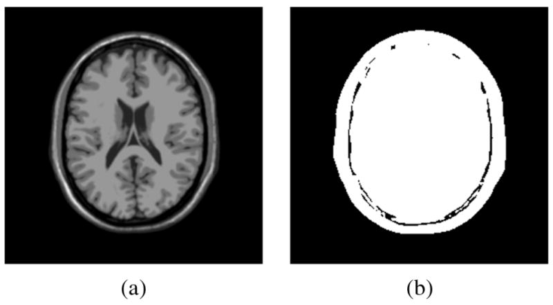
Synthetic experiments. (a) Original image (from BrainWeb) used in the synthetic experiments. (b) Mask used in the quality measures.

$$\text{SNR}(dB)=10{log}_{10}\left(\frac{S^2}{{\sigma }_n^2}\right)$$ (19)

where S is a measure for the signal intensity and ${\sigma }_n^2$ is the noise variance. The signal to noise ratios considered for the following experiments are given in Table I.

TABLE I.

Values of σ_n Used in the Synthetic Experiments. For the SNR the Mean Value of S in Each Region has Been Considered

σn	SNR (White Matter)	SNR (Gray Matter)	SNR (CSF)
5	30 dB	26 dB	17 dB
10	23.6 dB	20 dB	11 dB
20	17.6 dB	13.9 dB	5 dB

The noisy image is processed using eight different techniques (see Section II-B for details on these techniques); techniques taking into account the Rician Model: 1) the conventional approach by McGibney et al. [6]; 2) the ML estimator [7]–[10]; 3) the EM method [11], [12]; 4) the analytically exact solution, proposed by Koay and Basser in [19]; 5) the LMMSE estimator, as proposed in (14); 6) the RLMMSE estimator using 8 and 50 iteration steps, as proposed in (18); and (to compare the filters with other well-known techniques) techniques using a Gaussian noise model: 7) Gaussian smoothing, using a 11×11 kernel with σ = 1.5; and 8) adaptive Wiener filtering [25], using a 5×5 neighborhood. In order to achieve the best performance of the filter, σ_n is manually set to the actual value.

In all the cases where the variance of noise is needed, it is manually set to its optimal value. Note that the ML and EM estimators, as well as the method by Koay and Basser are designed to work with several samples of the same image. As in the present experiment we suppose only one sample is available, the statistics are computed using local neighborhoods. In all cases 5×5 neighborhoods have been used.

To compare the restoration performance of the different methods, two quality indexes are used: the structural similarity (SSIM) index [31] and the quality index based on local variance (QILV) [32]. Both give a measure of the structural similarity between the ground truth and the estimated images. However, the former is more sensitive to the level of noise in the image and the latter to any possible blurring of the edges. Both indexes are bounded; the closer to one, the better the image. The mean square error (MSE) is also calculated. These three quality measures are only being applied to those areas of the original image greater than zero [see Fig. 1]; this way the background is not taken into account when evaluating the quality of each method.

Table II shows the experimental results. Some graphical results for σ_n = 10 are shown in Fig. 2.

TABLE II.

Quality Measures: SSIM, QILV, and MSE for the Images in the Experiments. Best Value of Each Column is Highlighted. LMMSE-Based Schemes Show Better Results in Terms of Noise Removal and Edge Preservation

	σn =5			σn = 10			σn = 20
	SSIM	QILV	MSE	SSIM	QILV	MSE	SSIM	QILV	MSE
Noisy	0.9235	0.9977	24.8971	0.7904	0.9890	100.2940	0.5722	0.9251	395.0881
CA	0.8544	0.6394	190.9824	0.8491	0.6430	192.1922	0.8236	0.6543	205.6214
EM	0.5726	0.0140	2839.1	0.8685	0.6513	144.1177	0.8373	0.6342	168.0615
Koay	0.8797	0.6590	137.6257	0.8854	0.6856	133.9855	0.8280	0.5527	179.0641
ML	0.3770	0.2265	2120.9	0.8681	0.6516	144.2500	0.8370	0.6354	168.1712
Gaussian	0.8904	0.6479	128.5180	0.8789	0.6073	139.1106	0.8392	0.5145	190.3817
Wiener	0.9664	0.9967	18.1872	0.9092	0.9839	57.9197	0.8146	0.9076	161.8120
LMMSE	0.9681	0.9980	17.7973	0.9168	0.9921	53.9731	0.8346	0.9613	130.5361
RLMMSE (8)	0.9713	0.9981	17.4090	0.9270	0.9917	51.8197	0.8597	0.9502	122.5699
RLMMSE (50)	0.9714	0.9982	17.4562	0.9298	0.9915	51.8487	0.8540	0.9429	129.5132

Fig. 2.

Experiment with synthetic noise. MRI from Brainweb (Detail). (a) Original Image. (b) Image with Rician noise with σ_n = 10. (c) Gaussian filtered. (d) Conventional approach. (e) ML estimator. (f) EM method. (g) Koay’s method. (h) LMMSE estimator. (i) Recursive LMMSE (eight iterations). The LMMSE filters with correct noise estimation show the best performance, as confirmed by the numerical results in Table II.

When compared with other schemes considering a Rician noise model, the LMMSE and the RLMMSE show a better performance in terms of noise cleaning (a larger SSIM) while the edges are preserved (the QILV value gets better). The noise cleaning performance of the ML, EM, and Koay schemes are good, but, as the QILV index points out, they cause image blurring. Consequently, image information is lost at the border and the image edges. This performance is not due to the schemes themselves, but to the fact that they are originally designed to estimate the signal from multiple samples. When only one image is available, the statistics must be calculated locally. Consequently this local estimation produces some edge smoothing, in some cases similar to the one produced by a Gaussian filter. LMMSE, although it is also based on local statistics does not show this edge-blurring behavior.

The Gaussian smoothing, as expected, improves the quality of the image from an SSIM point of view, but the QILV suggests structural distortion due to blurring. In our experiments we also observed some numerical stability problems with EM and ML when the level of noise is low. Strikingly, all schemes, except for the proposed LMMSE approaches and the Wiener filter, fail when the level of noise is low: in this case, the quality indexes are lower than the corresponding quality indexes for the noisy image.

It is interesting to study the performance of the Wiener filtering; although it slightly blurs the image, it shows an overall good performance. Its performance is worse than the LMMSE, because the Wiener filter is based on a Gaussian noise model. This mismatch between the Rician model and the Gaussian model is not too large in structural MRI, but becomes more important for diffusion weighted images, where dark regions (where the mismatch is greatest) indicate large diffusion.

Finally, the RLMMSE results shows very good performance, when compared with the other schemes. There is a good balance between noise cleaning (SSIM index) and edge and structural information preservation (see QILV values). In addition, the filter shows great numerical stability: after 50 iterations the results are similar to those after eight iteration, indicating that the filter reaches a steady state.

One main advantage of the LMMSE filter (and to some extent for the RLMMSE filter) is that the solution can be computed in one single step (or a few steps for the RLMMSE filter), making it computationally efficient for large data sets as frequently encountered in DWI. This is in contrast to the EM and ML schemes, as well as to the approach by Koay and Basser, where the solution is found by numerical optimization and thus iteratively. As an illustration, in Table III runtimes for the LMMSE, the RLMMSE, and the EM algorithm as well as for the method by Koay are compared. All algorithms were implemented in Matlab. Reported execution times are measured by Matlab. Of note, while implementations of the LMMSE, the RLMMSE, and the EM algorithm could easily take advantage of Matlab’s efficient matrix computations, we used loops in the implementation of Koay’s method which may have increased computational time slightly. The timing experiments clearly demonstrate the efficiency of the LMMSE and the RLMMSE approach. An in-depth execution profile analysis shows the evaluation of Bessel functions (as required by the EM algorithm and the approach by Koay) to be costly.

TABLE III.

Execution time per slice (in seconds) of some filtering methods

	σn = 5	σn = 10	σn = 20
LMMSE	0.06	0.06	0.06
RLMMSE (8)	0.57	0.57	0.57
EM	28.13	28.08	20.61
Koay	145.6	150.4	155.4

A subset of the analysis is performed using real structural MR images. Since in this case the ground truth is unknown, the comparison is done strictly visually. A coronal slice from a 3-D structural MRI volume² was selected. The original image, see Fig. 3(a), exhibits noise. See Fig. 4 for a zoomed-in view. The image is filtered using the LMMSE and the RLMMSE estimators using the noise estimator given in (6). Results are shown in Fig. 3, details in Fig. 4. For comparison the same image is filtered using the conventional approach, EM estimation, and the method proposed by Koay and Basser. In all the cases adaptive noise estimation is performed using (16) with a 5×5 window.

Fig. 3.

Coronal slice from a 3-D acquisition. (a) Original image. (b) Conventional approach. (c) EM method. (d) Koay’s method. (e) LMMSE estimator, adaptive noise estimation using the local mean and a 5×5 window. (f) RLMMSE estimator, adaptive noise estimation using the local mean and a 5×5 window (eight iterations).

Fig. 4.

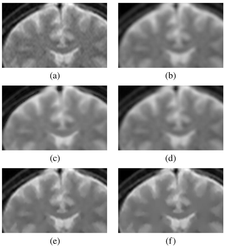
Detail of the images of the experiment of Fig. 3. (a) Original. (b) CA. (c) EM. (d) Koay. (e) LMMSE. (f) RLMMSE (eight steps).

As expected, the visual results are much better for the LMMSE and the RLMMSE estimators. The behavior shown for the other schemes is consistent with the synthetic experiments: noise is attenuated at the cost of blurring the image.

B. Filtering of Diffusion Weighted MR Images

This section investigates the performance of the proposed scheme when filtering DWI data. We use a SENSE EPI data set [33]: Scanned in a 3.0-T GE system, with 51 gradient directions (distributed on the sphere using the electric repulsion model with antipodal pairs), and eight baselines; voxel dimensions: 1.7 × 1.7 × 1.7 mm.

In areas with high diffusion along the gradient direction, the DWIs show a low signal level. Frequently, these areas are of great interest, since the direction of high diffusion is related to tissue structure [4]. However, they are also the most prone to noise effects and have the lowest signal to noise ratios. While Gaussian noise assumptions may suffice largely for nondiffusion-weighted images with high signal intensities (and consequentially high SNR), Rician noise models become more important for DWI, where dark signal areas are of higher importance.

All the DWIs are filtered using the RLMMSE filter and the noise estimator of (16). One of the advantages of this noise estimator is that no segmentation of the background is needed, neither manually nor automatic. This advantage is important when processing MR data in which an artificial background has been added.

Fig. 5(a) shows an EPI slice image. Fig. 5(b) shows in black all pixels with intensities equal to zero. Comparing both images, it is clear that there is a small area between the skull and the zero-background which corresponds to the actual background, and a greater area where an artificial zero background has been added. If the noise is estimated over the whole background there will clearly be a bias.

Fig. 5.

(a) Baseline image. (b) Thresholded image; in black all the pixels with intensity value equal to 0. An artificial black background has been added.

We can overcome this problem by using the local mean distribution. For the whole baseline volume, this distribution is depicted in Fig. 6(a). Due to the intensities that have been set to zero in the background, the maximum of the distribution is at the origin. However, it is still possible to identify a second maximum due to the noise itself. If the zero value pixels are not considered for the distribution, the histogram changes shape as shown in Fig. 6(b), and its maximum clearly reflects the noise level, in the same way as in (16). We will thus not consider zero value pixels for the noise estimation. (Note that alternatively, the estimation may be done using (17) for the pixels inside the head.)

Fig. 6.

Local mean distribution of a 3-D MR volume. (a) Distribution using all the values. (b) Distribution using only the points with intensities greater than 0 (the artificial background is not considered).

The whole EPI data set is filtered using this noise estimator and the RLMMSE filter. The noise is reestimated in each iteration. Fifteen iterations are considered (in all the cases with 15 iterations, the output reaches a steady state). Results of this filtering for different neighborhoods are shown in Fig. 7 (baseline) and Fig. 8 (DWI). For both, the baseline and the DWIs, the RLMMSE filter performs well in terms of noise removal while preserving image structure. The filtering effect is stronger for low signal intensity areas of the DWIs, since these are the areas most prone to noise according to the Rician noise model.

Fig. 7.

Slice 40 of the EPI dataset. Baseline. Original image and images filtered with different neighborhoods. Noise estimated over a (7,7,1) neighborhood. (a) Original baseline. (b) (3,3,1). (c) (5,5,1). (d) (7,7,1). (e) (9,9,1). (f) (11,11,1).

Fig. 8.

Slice 40 of the EPI dataset. DWI. Original image and images filtered with different neighborhoods. Noise estimated over a (7,7,1) neighborhood. (a) Original DWI. (b) (3,3,1). (c) (5,5,1). (d) (7,7,1). (e) (9,9,1). (f) (11,11,1).

C. Tensor Estimation

Diffusion weighted images are acquired to investigate the diffusion characteristic of water molecules which is in turn related to the underlying tissue microstructure. One of the simplest diffusion models is the diffusion tensor model which assumes a multivariate Gaussian probability density function for the water displacement. Since tensor estimation results are noise-dependent, noise removal before tensor estimation should lead to improved tensor estimation results.³

Assuming a multivariate Gaussian probability density distribution for the water displacement, the set of diffusion weighted images {A_k} acquired with gradient directions {g_k}, using a b-value b, is related to the nondiffusion-weighted baseline image A₀ through the Stejskal–Tanner equation [35], [36]

$$A_k=A_0{e}^{-b{\mathit{g}}_k^{T}T{\mathbf{g}}_k},$$ (20)

where T denotes the diffusion tensor. This images are corrupted with Rician Noise. If we further assume that our proposed estimation method removes (or at least significantly reduces) the noise from the diffusion weighted images, (20) may be written as

$${\widehat{A}}_k={\widehat{A}}_0{e}^{-b{\mathbf{g}}_k^{T}T{\mathbf{g}}_k}$$

and subsequently to

$$log\left(\frac{{\widehat{A}}_k}{{\widehat{A}}_0}\right)=-b{\mathbf{g}}_k^{T}T{\mathbf{g}}_k$$

which is linear in T and can be solved by least-squares. (We will only use least-squares tensor estimation in this paper, since it is unclear at this point what noise model should be used for tensor estimation after noise “removal” in the DWI domain.)

A variety of scalar measures have been defined for diffusion tensors [36], most prominently fractional anisotropy, which is proportional to the ratio of the Frobenius norms of the tensor deviatoric and the tensor itself [37]. While some of the measures may be computed without an explicit computation of the tensor eigenvalues, rotationally invariant measures may be written in terms of the tensor eigenvalues. To study the effect of the filtering on these eigenvalues, we created two different synthetic data sets, one 2-D and the other 3-D.

A synthetic 128×128 2-D tensor field was created; see Fig. 9(a) where tensors are depicted using ellipses [36]. The eigenvalues were chosen as

Fig. 9.

Synthetic vector field used in the experiments. σ_n = 100 (SNR = 2.62 dB), five different gradients. (a) Original tensor field. (b) Noisy. (c) Gaussian. (d) Wiener. (e) LMMSE. (f) RLMMSE (5).

$$\begin{array}{l}\mathbf{\lambda }=\{[1.9·{10}^{-3},0.4·{10}^{-3}],[2·{10}^{-3},0.1·{10}^{-3}],\\ [2·{10}^{-3},2·{10}^{-3}]\}\end{array}$$

and the diffusion weighted images were simulated using the Stejskal–Tanner (20). We consider different numbers of gradients (antipodal pairs uniformly distributed on the unit circle) and use a constant baseline image with signal intensity 1000. The DWIs are corrupted with Rician noise, Fig. 9(b), and the tensors are reestimated, using the least squares approach. Different values of σ_n were used.

Four restoration methods were applied to the noisy DWIs.

1. Gaussian smoothing, using a 11×11 kernel with σ = 1.5. This method was chosen to illustrate the effect of the smoothing on the DWI. As it was shown in Section III-A, some Rician-based methods also exhibit this behavior.

2. Adaptive Wiener filtering, using a 7×7 neighborhood, and manually setting σ_n to its actual value. This method was chosen because it showed a similar behavior to the LMMSE in structural MRI filtering.

3. LMMSE estimation, using a 7×7 neighborhood and manually setting σ_n to its actual value.

4. RLMMSE filtering with a 7×7 neighborhood, five iterations. As there is no background present, the noise is estimated over the DWIs using (17).

For the experiments we consider 3, 5, and 15 gradient directions and σ_n ∈ [30, 210]. To calculate the SNR we use (19), and define the power of the signal as

$$S^2=min(S_{i,j,k}^2).$$

We obtain S² = 1.83 · 10⁴. The error is defined as the absolute distance of the estimated eigenvalues to the original values. For each number of gradients and each σ_n the average of 100 experiments is considered. In Fig. 10 the mean and the standard deviation of the error are shown. In all cases, the estimation bias is smaller when using the LMMSE filter. The variance of the estimation, though also small is slightly larger than for the Wiener filtering, though the latter shows a greater bias. The RLMMSE shows a smaller bias but a greater variance than the other filtering methods.

Fig. 10.

Mean (left) and standard deviation (right) of the error of estimation of the eigenvalues for 3, 5, and 15 gradient directions. (a) Mean of the error, 3 directions. (b) Standard deviation of the error, 3 directions. (c) Mean of the error, 5 directions. (d) Standard deviation of the error, 5 directions. (e) Mean of the error, 15 directions. (f) Standard deviation of the error, 15 directions.

As an illustration, results for σ_n = 100 (SNR = 2.62 dB) and five different gradients are shown in Fig. 9 (tensor field) and in Fig. 11 where the distribution of the eigenvalues is depicted in a 2-D histogram. The original eigenvalues are depicted as a green dot. These figures lead to similar conclusions. Notice that the LMMSE histogram is practically centered in the original values, while the Wiener and Gaussian ones are biased, i.e. there is an underestimation of the principal eigenvalue. In addition, the Gaussian output [Fig. 11(b)] shows more clusters than centroids, as a consequence of the soft transition at the boundaries. These soft transitions (banding artifacts) can be observed in Fig. 9 and are caused by the Gaussian smoothing which tries to reconcile tensors that are spatially close, but have vastly different shapes and orientations.

Fig. 11.

Two dimensional histograms of the distribution of the estimated eigenvalues. σ_n = 100 (SNR = 2.62 dB). Five different gradients. In green the original eigenvalues. The proposed methods (LMMSE and RLMMSE) show a smaller bias in the estimation. (a) Noisy. (b) Gaussian. (c) Wiener. (d) LMMSE. (e) RLMMSE (five steps).

The next experiment tests the ability of the filter to correct the eigenvector direction. Specifically in this experiments we focus on the direction of the first eigenvector. A new synthetic 128 × 128 2-D tensor field was created—now without isotropic areas; see Fig. 12 where tensors are depicted using ellipses. We consider five gradients, a constant baseline image with signal intensity 1000 and Rician noise with σ_n = 100. The tensors are estimated, using the Least Squares approach. The noisy DWIs are filtered using a LMMSE filter and Gaussian smoothing. Results are shown in Fig. 13; 100 different realizations have been considered. The histogram normalized by its maximum value is depicted. The LMMSE is able to reduce the variance of estimation in the direction of the eigenvector. Notice that the Gaussian filter distribution shows some lobules between the actual vales. They are due to the fact that this filtering makes soft transitions between vectors that translate into intermediate orientations.

Fig. 12.

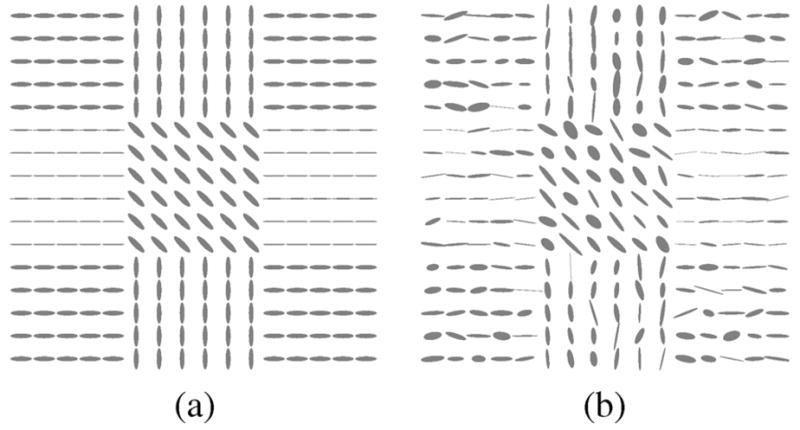
Synthetic 2-D tensor field for the eigenvector experiment. (a) Original. (b) Noisy.

Fig. 13.

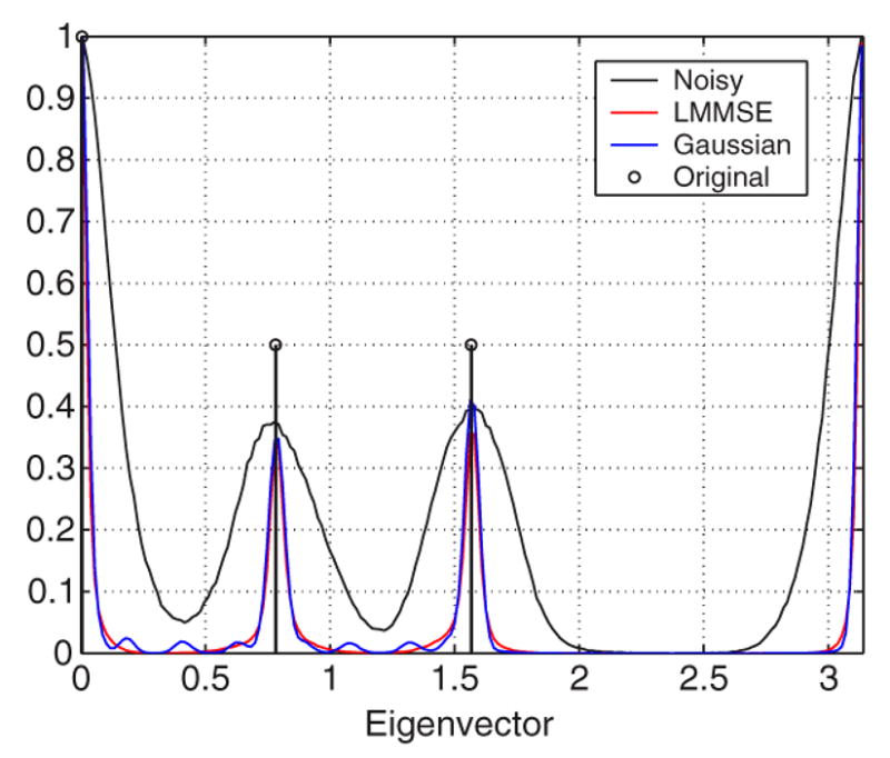
Original eigenvector direction (bold). Normalized histogram for the angle distribution of the eigenvectors of the noisy tensor field (black), after LMMSE estimation (red), and after Gaussian smoothing (blue).

To validate the method on a 3-D dataset, we created a synthetic diffusion weighted image volume modeling a 3-D logarithmic spiral. The core of the created bundle is parametrized by

$$x(p)=(a{e}^{bp}cospa{e}^{bp}sinpcp)$$ (21)

with a = 40, b = −0.05, c = 3. This results in a spiral with radius 40 for p = 0 which gets tighter and tighter with increasing p and thus models fiber bundles of different curvatures (see Fig. 14). At every point p of (21) we use the Frenet trihedron induced by the Frenet equations [38] to orient a tensor T in space (where the tangent direction is aligned with the major eigenvector of T and the binormal direction is associated with the minor eigenvector of T). The eigenvalues of T were chosen as λ_i = {6 · 10⁻³, 2 · 10⁻³, 10⁻³} and the diffusion weighted images were simulated using the Stejskal–Tanner equation. We used the same 51 gradient directions and eight baseline scheme as for the real echo planar images. The resulting synthetic volume is of dimension 128 × 128 × 100 with isotropic voxels of side length 1 mm. To create tensor values away from the core parametrized by (21), voxels were assigned the closest tensor on the core. The trace of the tensors was scaled based on this closest distance to the core. Voxels at a distance larger than 5 mm were assigned the zero tensor, voxels closer than 3 mm were assigned the original closest tensor on the core. Voxels in between were weighted using a Gaussian with standard deviation of one.

Fig. 14.

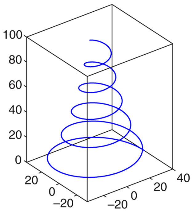
Logarithmic spiral.

Rician noise with σ = 70 was added to the noise-free diffusion weighted images. The diffusion weighted images were then filtered for 15 iterations with the RLMMSE filter (with 7×7 axial filtering and estimation neighborhoods), as well as with a Gaussian filter with a standard deviation of 1.5.

Figs. 15 and 16 show the spectral deviations (i.e., the differences of the estimated eigenvalues to the nominal eigenvalues) to the synthetic groundtruth for the proposed method and the Gaussian filter. All results were obtained after applying a mask, removing all tensors with a trace smaller than 0.001. The RLMMSE results are clearly superior to Gaussian smoothing. The estimation of the principal eigenvalue is greatly improved and the overall estimation is less biased.

Fig. 15.

Logarithmic histogram of spectral deviations with respect to the ground truth for different filtering methodologies (Gaussian and RLMMSE) with subsequent linear tensor estimation. The proposed method leads to a much better estimation of the tensor eigenvalues. (a) Largest eigenvalue. (b) Mean of two smallest eigenvalues.

Fig. 16.

Two-dimensional logarithmic histograms of spectral deviations with respect to the ground truth for different filtering methodologies (Gaussian and RLMMSE; the axes are mean of the smallest eigenvalues over the major eigenvalue). The proposed method leads to a much better estimation of the tensor eigenvalues. (a) Noisy. (b) Filteres. (c) Gauss filtered.

D. DWI Filtering and DTI Applications

To conclude the results section we show some examples of the qualitative performance of the LMMSE estimator for different DTI applications. We use the real data volume of Section III-B. The following experiments were performed.

• Fractional anisotropy and main eigenvector computation. In Fig. 17 we show the FA and the main eigenvector scaled by the main eigenvalue of both the original data set and the data set after 10 iterations of the RLMMSE using a 7×7 neighborhood. The RLMMSE filter results in a regularization of the vector directions.

• Color by orientation computation. Fig. 18 shows the orientation of the first eigenvector using color coding, for two different slices of the volume, for both the original data and the data after an LMMSE filtering using a 7 × 7 neighborhood. In this case RED means anterior–posterior direction (X axis), GREEN left–right (Y axis), and BLUE inferior–superior (Z axis). Results indicate a clear reduction of the noise without significant loss of structure.

• Tractography computation. We performed tractography for the Uncinate Fasciculus, starting in the same seed-point for both the original data set and the data set filtered using LMMSE (7 × 7 neighborhood). Results are shown in Fig. 19. Fig. 19 demonstrates the advantage of the noise reduction procedure in tracing the Uncinate Fasciculus. Anatomically, this fiber bundle has a U-like shape, and connects orbital frontal with anterior temporal regions. Fig. 19(a) shows results of tractography on unfiltered data, where tracts originating from the frontal lobe are mostly terminating before they curve and cross the temporal stem into the temporal lobe. Fig. 19(b) shows that after noise reduction, the Uncinate Fasciculus tracts are continuing all the way into the temporal lobe. Not only are fibers on average longer and have a more homogeneous distribution after filtering, but they are also more anatomically correct.

Fig. 17.

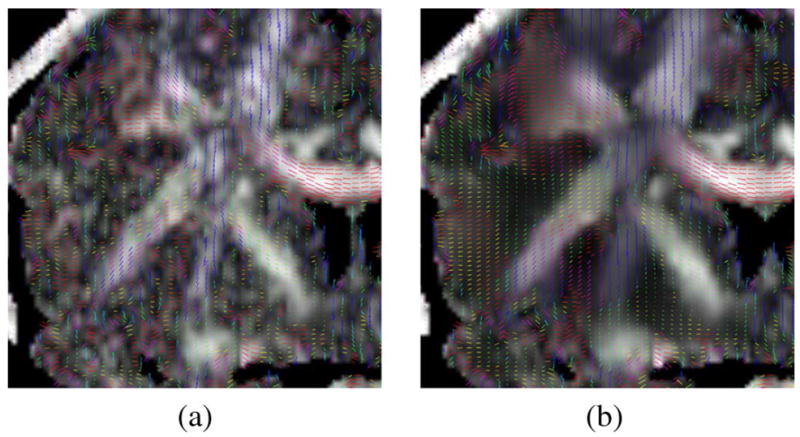
Main eigenvector over fractional anisotropy. The filtered vector field is more homogeneous than the noisy one. (a) Original volume. (b) RLMMSE (10 iterations).

Fig. 18.

DTI data, color by orientation of the main eigenvector, two different slices. RED means anterior–posterior direction (X axis), GREEN left–right (Y axis) and BLUE inferior–superior (Z axis). Original data (left) and after LMMSE filtering (right), (a) Original, (b) LMMSE. (c) Original, (d) LMMSE.

Fig. 19.

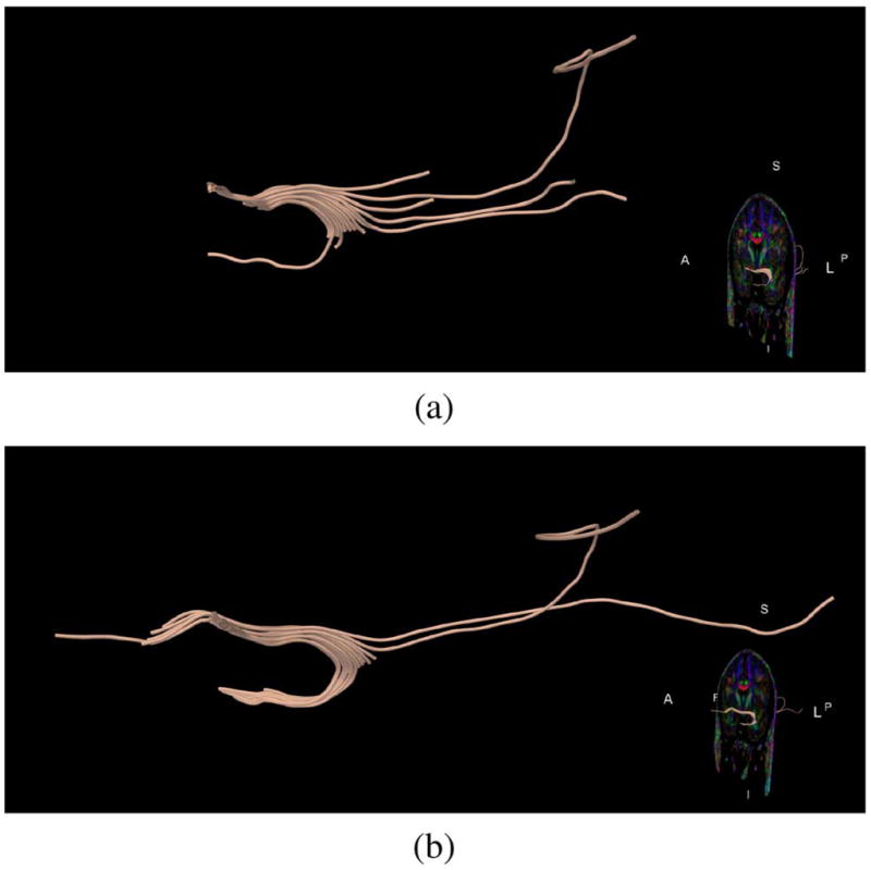
Automatic tractography of the Uncinate Fasciculus. Tractography on the filtered data set follows the shape of the bundle better, (a) Original data, (b) Data after filtering.

IV. Conclusion

This paper introduces a one-step and a recursive LMMSE estimator for signal estimation and noise removal in magnetic resonance images assuming a Rician noise model. Unlike other existing schemes, the LMMSE has a closed-form expression, is computationally efficient, easy to use and easy to implement.

Various validation experiments have been performed and the filter has been tested against a number of competing techniques. Diffusion information is based on the interplay between diffusion weighted images with a corresponding baseline image, thus validation was performed using real and synthetic data for diffusion weighted magnetic resonance images as well as for structural magnetic resonance images.

Structural similarity and quality index tests revealed superior image denoising results for the LMMSE estimators in comparison to a set of competing methods: overall noise was reduced while keeping structural information and minimizing blurring effects. All testing was performed assuming that only one measurement realization is available for each voxel, a scenario that the LMMSE estimators are designed for, but which puts methods designed for multiple acquisitions at a disadvantage. However, this is an important scenario, especially when considering diffusion weighted image acquisitions with high angular and spatial resolution where overall acquisition time may become an issue. The LMMSE estimators led to qualitatively good results for the diffusion weighted images themselves as well as for derived quantities (such as FA images and tractography results). Further, a testing of the proposed filtering methodology on synthetic DWI datasets showed significant reductions in estimation bias for the tensor spectrum as well as a beneficial smoothing effect on the tensor field.

A possible future extension would be an anisotropic Rician LMMSE scheme in analogy to the recent approach by Martin–Fernandez et al. [17] as well as an in-depth investigation into the noise-properties of the filtered image data.

Appendix A About the RLMMSE

One important issue in the RLMMSE definition is how long the assumption of Rician distributed data may hold when recursive filtering is considered. A priori, nothing assures that the data remains Rician once filtered. To test the filter behavior, we corrupted a 256 × 256 constant image of value 100 with Rician noise with σ_n = 40. To study the evolution of the distribution, the image is filtered with a LMMSE estimator using σ_n/2 instead of σ_n. This way, the image is not totally denoised. Five iterations are performed, and after each one the value of the noise variance is reestimated. Results are depicted in Fig. 20, where the actual distribution of the data is compared with the Rician distribution and Gaussian distribution for each iteration.

Fig. 20.

Experiment with synthetic noise, (a) Original, (b) One iteration ( $\widehat{{\sigma }_n}=26$). (c) Two iterations ( $\widehat{{\sigma }_n}=18$). (d) Three iterations ( $\widehat{{\sigma }_n}=15$). (e) Four iterations ( $\widehat{{\sigma }_n}=12$). (f) Five iterations ( $\widehat{{\sigma }_n}=9$).

There is a slight mismatch with increasing numbers of iterations, but the Rician assumption is still reasonable. Furthermore, when the SNR gets smaller, the Rician and Gaussian converges as expected for high SNR values.

This is similar to the Gaussian distribution, but not exactly the same.

Another important issue for the RLMMSE is the stability of the K parameter, which is defined as [see (15)]

$$K=1-\frac{4{\sigma }_n^2(\langle M^2\rangle -{\sigma }_n^2)}{\langle M^4\rangle -{\langle M^2\rangle }^2}.$$

Taking into account that [28]

$$\begin{array}{l}E\{M^2\}=E\{A^2\}+2{\sigma }_n^2\\ E\{M^4\}=E\{A^4\}+8{\sigma }_n^{2}E\{A^2\}+8{\sigma }_n^4\end{array}$$

this equation may be rewritten as a function of the original data

$$\begin{array}{l}K=\frac{E\{A^4\}-E{\{A^2\}}^2}{E\{A^4\}-E{\{A^2\}}^2+4{\sigma }_n^2(E\{A^2\}+{\sigma }_n^2)}\\ =\frac{\text{Var}(A^2)}{\text{Var}(A^2)+4{\sigma }_n^2(E\{A^2\}+{\sigma }_n^2)}.\end{array}$$

In the uniform areas of the original image the variance is very small or zero, i.e. Var(A²) → 0, and accordingly K → 0 and

$$\widehat{A^2}=E\{M^2\}-2{\sigma }_n^2=E\{A^2\}.$$

The estimator for the uniform areas is just the mean. On the other hand, when the level of noise is very low, i.e. ${\sigma }_n^2\to 0$ then K → 1, and therefore

$$\widehat{A^2}=M^2.$$

If no noise is present, the estimator is the image itself. One problem may arise if both Var(A²) and ${\sigma }_n^2$ tend to 0. However, in that case, both estimators are correct, so, in a uniform area

$$\widehat{A^2}=M^2=E\{M^2\}-2{\sigma }_n^2=E\{A^2\}=E\{M^2\}.$$

In practical experiments, there can be cases in which, due to numerical artifacts, K is negative; this may be more common when the real image does not completely follow the Rician model. In this case it is useful to add the following restriction:

$$K=max\{K,0\}.$$

Appendix B About the Noise Estimators

Both noise estimators used in this paper have been previously introduced and studied in [28]. For the sake of completeness, a brief explanation of them is included in this appendix.

Due to the influence of the pixels in the background of an MR image, the local mean distribution of a nonnoisy MRI presents a maximum around zero (see Fig. 21(a), solid line). When the image is corrupted with Rician noise, this maximum is now shifted to a value related to σ_n [see the dotted line in Fig. 21(a)]. As the mean of a Rayleigh distribution is defined as ${\mu }_1={\sigma }_n\sqrt{\pi /2}$, we can define a σ_n estimator

$$\widehat{{\sigma }_n}=\sqrt{\frac{2}{\pi }}argmax\{p(\widehat{{\mu }_1})\}$$

where $p(\widehat{{\mu }_1})$ the distribution of the sample local mean. The maximum may be calculated as the mode of the distribution

$$\widehat{{\sigma }_n}=\sqrt{\frac{2}{\pi }}\text{mode}({\widehat{{\mu }_1}}_{i,j})=\sqrt{\frac{2}{\pi }}\text{mode}(\langle I_{i,j}\rangle ).$$ (22)

This assumption can be proved by analyzing the mode of the distribution of the mean of Rayleigh random variables. The sum of Rayleigh variables is a classical problem in communications. Some approximations are usually employed, as the one in [39].

The effect of changing the size for the window used for estimation [see Fig. 21(b)] is a change in the width of the distribution, but in any case, the maximum stays at the same value. Accordingly, the mode does not change and neither does the estimation.

The starting point of the variance-based estimator is that, if no texture is present, the distribution of the local variances of an image will have its maximum value around zero. With this assumption in mind, we will first approximate the variance of a Rician model as

$${\sigma }_M^2\approx {\sigma }_n^2\left(1-\frac{5}{4}\frac{{\sigma }_n^4}{A^2}-\cdots \right).$$

If $E\{A_{ij}^2\}>{\sigma }_n^2$, and even if $E\{A_{ij}^2\}\gg {\sigma }_n^4$ we can say that

$${\sigma }_{M_{ij}}^2\approx {\sigma }_n^2$$

and accordingly, if the variance of the signal is estimated locally, the variance of noise can be estimated as

$${\widehat{\sigma }}_n^2=\text{mode}\left({\sigma }_{M_{ij}}^2\right).$$

This is similar to considering the rough approximation of the noise being Gaussian when the SNR is high. This way, the sample variance has a gamma distribution with mode

$$\text{mode}({\sigma }_M^2)={\sigma }_n^2\frac{N-3}{N-1}.$$

To completely justify this result, the distribution of the sample variance for the Rician model must be calculated.

References

- 1.Kubicki M, McCarley RW, Westin CF, Park HJ, Maier S, Kikinis R, Jolesz FA, Shenton ME. A review of diffusion tensor imaging studies in schizophrenia. J Psychiatry Res. 2005;41(1–2):15–30. doi: 10.1016/j.jpsychires.2005.05.005. [DOI] [PMC free article] [PubMed] [Google Scholar]
- 2.Srinivasan A, Goyal M, Azri FA, Lum C. State-of-the-art imaging of acute stroke. Radio Graph. 2006;26:S75–S95. doi: 10.1148/rg.26si065501. [DOI] [PubMed] [Google Scholar]
- 3.Hsu EW, Muzikant AL, Matulevicius SA, Penland RC, Henriquez CS. Magnetic resonance myocardial fiber-orientation mapping with direct histological correlation. Amer J Physiol Heart Circulatory Physiol. 1998;274:1627–1634. doi: 10.1152/ajpheart.1998.274.5.H1627. [DOI] [PubMed] [Google Scholar]
- 4.Beaulieu C. The basis of anisotropic water diffusion in the nervous system—A technical review. NMR Biomed. 2002;15:435–455. doi: 10.1002/nbm.782. [DOI] [PubMed] [Google Scholar]
- 5.Henkelman RM. Measurement of signal intensities in the presence of noise in MR images. Med Phys. 1985;12(2):232–233. doi: 10.1118/1.595711. [DOI] [PubMed] [Google Scholar]
- 6.McGibney G, Smith MR. Unbiased signal-to-noise ratio measure for magnetic resonance images. Med Phys. 1993;20(4):1077–1078. doi: 10.1118/1.597004. [DOI] [PubMed] [Google Scholar]
- 7.Sijbers J, den Dekker AJ, Scheunders P, Van Dyck D. Maximum-likelihood estimation of Rician distribution parameters. IEEE Trans Med Imag. 1998 Jun;17(3):357–361. doi: 10.1109/42.712125. [DOI] [PubMed] [Google Scholar]
- 8.Sijbers J, Jden Dekker A, Van Dyck D, Raman E. Estimation of signal and noise from Rician distributed data. Proc. Int. Conf. Signal Process. Commun., Las Palmas de Gran Canaria; Spain. Feb. 1998; pp. 140–142. [Google Scholar]
- 9.Sijbers J, den Dekker AJ. Maximum likelihood estimation of signal amplitude and noise variance form MR data. Magn Reson Imag. 2004;51:586–594. doi: 10.1002/mrm.10728. [DOI] [PubMed] [Google Scholar]
- 10.Jiang L, Yang W. Adaptive magnetic resonance image denoising using mixture model and wavelet shrinkage. Proc. VIIth Digital Image Comput.: Tech. Appl.; Sydney, Australia. Dec. 2003. [Google Scholar]
- 11.DeVore MD, Lanterman AD, O’Sullivan JA. ATR performance of a Rician model for SAR images. Proc. SPIE 2000, ISSU 4050; Orlando, FL. Apr 2000; pp. 34–37. [Google Scholar]
- 12.Marzetta TL. EM algorithm for estimating the parameters of multivariate complex Rician density for polarimetric SAR. Proc ICASSP. 1995;5:3651–3654. [Google Scholar]
- 13.Nowak R. Wavelet-based Rician noise removal for magnetic resonance imaging. IEEE Trans Image Proccess. 1999 Oct;8(10):1408–1419. doi: 10.1109/83.791966. [DOI] [PubMed] [Google Scholar]
- 14.Pižurica A, Philips W, Lemahieu I, Acheroy M. A versatile wavelet domain noise filtration technique for medical imaging. IEEE Trans Med Imag. 2003 Mar;22(3):323–331. doi: 10.1109/TMI.2003.809588. [DOI] [PubMed] [Google Scholar]
- 15.McGraw T, Vemuri BC, Chen Y, Rao M, Mareci T. DT-MRI denoising and neuronal fiber tracking. Med Imag Anal. 2004;8:95–111. doi: 10.1016/j.media.2003.12.001. [DOI] [PubMed] [Google Scholar]
- 16.Ahn CB, Song YC, Park DJ. Adaptive template filtering for signal-to-noise ratio enhancement in magnetic resonance imaging. IEEE Trans Med Imag. 1999 Jun;18(6):549–556. doi: 10.1109/42.781019. [DOI] [PubMed] [Google Scholar]
- 17.Martin-Fernandez M, Aberola-Lopez C, Ruiz-Alzola J, Westin CF. Sequential anisotropic Wiener filtering applied to 3-D MRI data. Magn Reson Imag. 2007;25:278–292. doi: 10.1016/j.mri.2006.05.001. [DOI] [PubMed] [Google Scholar]
- 18.Basu S, Fletcher T, Whitaker R. Rician noise removal in diffusion tensor MRI. Proc MICCAI. 2006;1:117–125. doi: 10.1007/11866565_15. [DOI] [PubMed] [Google Scholar]
- 19.Koay CG, Basser PJ. Analytically exact correction scheme for signal extraction from noisy magnitude MR signals. J Magn Reson. 2006;179:317–322. doi: 10.1016/j.jmr.2006.01.016. [DOI] [PubMed] [Google Scholar]
- 20.Gudbjartsson H, Patz S. The Rician distribution of noisy MRI data. Magn Reson Med. 1995;34:910–914. doi: 10.1002/mrm.1910340618. [DOI] [PMC free article] [PubMed] [Google Scholar]
- 21.Drumheller DM. General expressions for Rician density and distribution functions. IEEE Trans Aerosp Electron Syst. 1993 Apr;29(2):580–588. [Google Scholar]
- 22.Simon MK. Probability Distributions Involving Gaussian Random Variables. Norwell, MA; Kluwer: 2002. [Google Scholar]
- 23.Sijbers J, den Dekker AJ, Van Audekerke J, Verhoye M, Van Dyck D. Estimation of the noise in magnitude MR images. Magn Reson Imag. 1998;16(1):87–90. doi: 10.1016/s0730-725x(97)00199-9. [DOI] [PubMed] [Google Scholar]
- 24.Sijbers J, Jden Dekker A, Poot D, Verhoye M, Van Camp N, Van der Linden A. Robust estimation of the noise variance from background MR data. Proc SPIE Med Imag 2006: Image Process. 2006:6144. [Google Scholar]
- 25.Lim JS. Two Dimensional Signal and Image Processing. Engle-wood Cliffs, NJ: Prentice Hall; 1990. [Google Scholar]
- 26.Kay SM. Fundamentals of Statistical Signal Processing: Estimation Theory. Englewood Cliffs, NJ: Prentice Hall; 1993. [Google Scholar]
- 27.Aja-Fernández S, Alberola-López C, Westin C-F. Proc MICCAI. New York: Springer; 2007. Signal LMMSE estimation from multiple samples in MRI and DT-MRI; p. 4792. Lecture Notes Computer Science. [DOI] [PubMed] [Google Scholar]
- 28.Aja-Fernández S, Alberola-López C, Westin CF. Noise and signal estimation in magnitude MRI and Rician distributed images: A LMMSE approach. IEEE Trans Image Proccess. 2008 Aug;17(8):1383–1398. doi: 10.1109/TIP.2008.925382. [DOI] [PubMed] [Google Scholar]
- 29.Collins DL, Zijdenbos AP, Killokian V, Sled JG, Kabani NJ, Holmes CJ, Evans AC. Design and construction of a realistic digital brain phantom. IEEE Trans Med Imaging. 1998 Jun;17(3):463–468. doi: 10.1109/42.712135. [DOI] [PubMed] [Google Scholar]
- 30.Oppenheim AV, Schafer RW. Discrete-Time Signal Processing. Englewood Cliffs, NJ: Prentice Hall; 1989. [Google Scholar]
- 31.Wang Z, Bovik AC, Sheikh HR, Simonceli EP. Image quality assessment: From error visibility to structural similarity. IEEE Trans Image Proccess. 2004 Apr;13(4):600–612. doi: 10.1109/tip.2003.819861. [DOI] [PubMed] [Google Scholar]
- 32.Aja-Fernández S, San-José-Estépar R, Alberola-López C, Westin C-F. Image quality Assesment based on local variance. Proc 28th IEEE Int. Conf. Eng. Med. Biol. Soc. (EMBC); New York. Sep. 2006; pp. 4815–4818. [DOI] [PubMed] [Google Scholar]
- 33.Bammer R, Auer M, Keeling SL, Augustin M, Stables LA, Prokesch RW, Stollberger R, Moseley ME, Fazekas F. Diffusion tensor imaging using single-shot SENSE-EPI. Magn Reson Med. 2002;48:128–136. doi: 10.1002/mrm.10184. [DOI] [PubMed] [Google Scholar]
- 34.Koay CG, Chang LC, Carew JD, Pierpaoli C, Basser PJ. A unifying theoretical and algorithmic framework for least squares methods of estimation in diffusion tensor imaging. J Magn Reson. 2006;182:115–125. doi: 10.1016/j.jmr.2006.06.020. [DOI] [PubMed] [Google Scholar]
- 35.Stejskal EO, Tanner JE. Spin diffusion measurements: Spin echoes in the presence of a time-dependent field gradient. J Chem Phys. 1965;42:288–292. [Google Scholar]
- 36.Westin CF, Maier SE, Mamata H, Nabavi A, Jolesz FA, Kikinis R. Processing and visualization for diffusion tensor MRI. Med Imag Anal. 2002;6:93–108. doi: 10.1016/s1361-8415(02)00053-1. [DOI] [PubMed] [Google Scholar]
- 37.Basser PJ, Pierpaoli C. Microstructural and physiological features of tissues elucidated by quantitative-diffusion-tensor MRI. J Magn Reson B. 1996;111(3):209–219. doi: 10.1006/jmrb.1996.0086. [DOI] [PubMed] [Google Scholar]
- 38.do Carmo MP. Differential Geometry of Curves and Surfaces. New York: Prentice Hall; 1976. [Google Scholar]
- 39.Beaulieu NC. An infinite series for the computation of the complementary probability distribution function of a sum of independent random variables and its application to the sum of Rayleigh random variables. IEEE Trans Comm. 1990 Sep;38(9):1463–1473. [Google Scholar]