Multiple indicator hidden Markov model with an application to medical utilization data

Abstract

Monthly counts of medical visits across several years for persons identified to have alcoholism problems are modeled using two-state hidden Markov models (HMM) in order to describe the effect of alcoholism treatment on the likelihood of persons to be in a “healthy” or “unhealthy” state. The medical visits can be classified into different types leading to multivariate counts of medical visits each month. A multiple indicator hidden Markov model is introduced that simultaneously fits the multivariate Poisson counts by assuming a shared hidden state underlying all of them. The multiple indicator hidden Markov model borrows information across different types of medical encounters. A univariate HMMs based on the total count across types of medical visits each month is also considered. Comparisons between the multiple indicator HMM and the total count HMM are made, as well as comparisons with more traditional longitudinal models that directly model the counts. A Bayesian framework is used for estimation of the HMM and implementation is in Winbugs.

1 Introduction

Medical encounter data has the potential to provide information useful for addressing questions regarding effectiveness of certain treatments at the population level. Using medical insurance records it is possible to collect the date when medical visits of certain types occurred for each individual in a target population over an entire target time period. Data of this type has been useful in the study of persons with alcoholism problems [1-7]. With this natural history data source it is possible to discern periods of time when the individual is engaging in insurance covered alcoholism treatment and also to determine how frequently the individual presents for different types of medical care. A model for these multivariate (i.e. multiple types of encounters) longitudinal (i.e. monthly) counts of medical visits for each patient can then be constructed and used to estimate the effect of treatment.

In the study of alcoholism, research has found [3-7] that people with alcoholism problems use medical care more often than the general population. In addition, there is a kind of on- and-off phenomena associated with alcoholism where individuals attempt to quit or control their drinking and then relapse or “fall off the wagon” and exhibit full blown problems [8-10]. Therefore, it is reasonable to hypothesize an unobserved health state that governs individual medical care usage with the normal rate of medical care use corresponding to a “Healthy” state and an excess medical care usage corresponding to “Unhealthy” state. The probability of being in the “Healthy” or “Unhealthy” health state for a particular person in a given month will differ depending on the past health state this person was in and other possible fixed and time varying covariates including specifically alcoholism treatment. The terms “Healthy” and “Unhealthy” are used throughout the current paper as labels for the two different states but it is important to point out that the two modeled states (in the hidden Markov models later to be described) more accurately reflect periods simply of high and low medical usage and thus are meant to be surrogates for the concepts of “Unhealthy” and “Healthy” respectively. As such there may be periods of highly frequent medical use corresponding to an “Unhealthy” state being predicted by the model that in the reality of the patient do not represent an “unhealthy” period in the person’s life and vica versa for low use and the “Healthy” state. A limitation of this sort of modeling based solely on insurance medical visit records is that the quality of this surrogacy cannot be verified.

In this paper we propose to model the “Healthy” and “Unhealthy” unobserved health states as a hidden Markov chain and since the observations are monthly counts of medical visits, a two state Poisson hidden Markov model (HMM) [11] is used. The major research question is whether alcoholism treatment reduces the probability of subsequently entering the “Unhealthy” state as measured by the medical encounters. The medical encounters can be collapsed as a total count for any given month regardless of what the reason for the visit is, or they can be organized into counts of different types of medical encounters. In the case of alcoholism patients, since we want to use medical visits as a surrogate for “unhealthy” periods, it is of interest to separate out the visits that are possibly related to different aspects of alcoholism. Hence if medical visits of those types are observed (even if they are not as numerous as other non-alcohol related encounters) it may make sense for the model to capture the period as “Unhealthy” since it contained alcoholism-type medical visits. The medical encounters are split into meaningful categories leading to multivariate counts of medical visits each month.

In this paper, we consider fitting the two state hidden Markov model to the total medical visits per month and we introduce a multiple indicator hidden Markov model that simultaneously fits the multivariate counts by assuming a shared hidden state underlying all of them. The multiple indicator hidden Markov model borrows information across different types of encounters.

Estimation of parameters for the HMM can proceed within a frequentist or Bayesian framework. Within the maximum likelihood framework, the EM algorithm, also known as the Baum-Welch algorithm in the HMM literature, can be implemented by treating the hidden states as missing values, implementing the forward backward recursion in the E-step and finding the value of the parameters that maximize the likelihood in the M-step [12-13]. Within the Bayesian Framework, the MCMC technique and Metropolis-Hastings Algorithms can be used to sample from the posterior distribution of the parameters [14]. Scott (2002) [15] pointed out that MCMC methods for HMM can also be improved by incorporating the forward-backward, likelihood and Viterbi recursive algorithms into the MCMC algorithm, improving convergence as well as computation effciency. While these algorithms can be incorporated to improve the computational effciency of the MCMC, it is important to note that the direct Gibbs sampling approach for the HMM is computationally very straightforward and intuitive. Moreover, direct Gibbs can be implemented in the existing Winbugs software. In this paper we work within a Bayesian framework and use Winbugs (and provide Winbugs code) for fitting the univariate and multiple indicator HMM models to the data.

A description of the data and motivation for the models are given in section 2. In section 3, the univariate two state Poisson HMM is described for the monthly number of total medical visits and the multiple indicator HMM is introduced for modeling the multiple types of encounters simultaneously. Section 4 presents the Bayesian inference, and the results for the data example are shown in section 5 along with a comparison to two other standard longitudinal models. That is, a Poisson lagged regression model is considered for the total medical visit data and a similar model using the regression method for multiple source data [16] is used for the data separated into different types of medical encounters. Finally, section 6 gives some discussion and ideas for future research.

2 Data and Model Motivation

The data come from a large managed behavioral and medical health care insurance company which provided alcoholism treatment records and medical encounter claims records. Altogether there were 29122 patients identified with alcoholism problems who had insurance coverage for at least 2 months during the time period from January 1993 to December 1999, details of the sample are given elsewhere, see [1]. All medical encounter claims during the study period for each of these 29122 patients were extracted. The medical encounters are separated into four types: 1. Alcohol Specific, this type includes those medical visits which are direct results of drinking alcohol (alcohol psychoses, alcohol dependence syndrome, alcohol abuse, poisoning by alcohol, toxic effects of alcohol), 2. Alcohol Chronic, which includes medical encounters that reflect a chronic condition commonly associated with alcoholism (e.g. cirrhosis, chronic pancreatitis, alcoholic myocardiopathy), 3. Alcohol Acute, this type includes acute medical conditions and accidents that might be attributed to active drinking (e.g. sprains, alcoholic gastritis, fracture, motor vehicle accident), and finally, 4. Not Alcohol, which includes all other medical encounters not captured in the other types. The total number of medical encounters for each of the types (Alcohol Specific, Alcohol Chronic, Alcohol Acute and Not Alcohol) was computed as the number of days in a particular month that an individual had an encounter of that particular type. It is possible for individuals to have multiple types of encounters in 1 day. There are 84 sequential months within the study period and daily data for each type of medical encounter for each patient are aggregated to the month level.

Of the 29122 patients identified to have alcoholism problems, 16053 were determined as having fully engaged in an alcoholism treatment program (9053 of them engaging exclusively in outpatient alcoholism treatment and the other 7000 engaging in alcoholism treatment that included at least some inpatient care). An episode of care methodology based on intensity of alcoholism treatment visits per month was used to define the alcoholism treatment period [17] which provides a clearly defined beginning and ending month of treatment. Alcoholism treatment typically lasts several months and the length and exact calendar months vary by patient. The remaining 13096 of the 29122 patients who were identified to have alcoholism problems but who did not fully engage in treatment will serve as the control group providing a background intensity rate of medical encounters during the same time period. Specifically an offset for each type of medical encounter is calculated using the mean of that type of medical encounter for the control group in each of the 84 months in the study.

The current study focuses on the 9053 patients who received outpatient alcoholism treatment. Among them, 69% were male and the mean age was 41 with a standard deviation of 10. The insurance company provides service nationally with 11% of these individuals from the Midwest, 12% from the North East, 35% from the South and 42% from the West. During the study period 4% (i.e. 362 of the 9053) of the individuals who engaged in outpatient alcoholism treatment had more than one distinct treatment episode. These patients are not considered separately and only their earliest observed treatment episode is entered into analysis. That is, the analysis investigates the overall effect of alcoholism treatment that pools together the effect seen in patients who may not return again for treatment with the likely poor effect seen in patients who do have multiple treatments.

The mean total number of medical encounters over the 84 month study period for the 9053 patients was 24.88 encounters per 100 person months. When this is split out by the type of encounters, the results are: Not Alcohol 20.43 per 100 persons per month, Alcohol Specific 1.25 per 100 persons per month, Alcohol Acute 2.88 per 100 persons per month and Alcohol Chronic 0.31 per 100 persons per month. As can be deduced from the overall low frequency of medical encounters, many individuals are having no medical encounters in many months, i.e. there are a lot of zero counts in the data. As the observed data represent counts of medical visits, direct modeling of the data via a Poisson distribution is natural to consider. A simple examination of the overdispersion parameter (Pearson Chi-square divided by degrees of freedom) associated with Poisson modeling of total visits controlling for the background rate (i.e. the offset value associated with control patients) finds a value of 3.75 indicating a high degree of lack of fit from the Poisson distribution. Thus, in conjunction with the large number of zero counts, a mixture of two Poisson distributions may be a more realistic match to this data: one with a very small mean (to capture the preponderance of zeros yet allowing some small number of non-zero counts) corresponding to encounters during a “Healthy” state and the other with a mean that captures larger counts while still allowing zeros thus corresponding to an “Unhealthy” state. This mixture of Poisson distributions is preferred over a zero-inflated Poisson due to the desire to allow for non-zero counts (albeit small) in the model for the “Healthy” state.

Exploratory investigation of the longitudinal nature of these data finds that individuals tend to have medical encounters in streaks or runs of months. In particular, the rate of transitioning to having any encounters in a given month given that there were no encounters in the previous month for each type of encounters are: Not Alcohol 0.41%, Alcohol Specific 0.36%, Alcohol Acute 1.25%, and Alcohol Chronic 0.08%. Whereas, the rate of having any encounters in a particular month given that there was at least one encounter of the same type in the previous month is: Not Alcohol 40.35%, Alcohol Specific 36.16%, Alcohol Acute 24.00%, and Alcohol Chronic 33.06%. Thus, there is a much higher probability of having any of the medical encounters in a given month when there was an encounter of the respective type in the previous month as compared to not having had an encounter of that type in the previous month. This month-to-month dependence may be reasonably captured using a Markov structure where the encounters in each month depend on the existence of an encounter in the previous month and other covariates.

Finally, it is of interest to examine the relationships among the 4 different types of encounters. Large associations (odds ratios) between any occurrence of the different types of medical encounters within any month are found and indicate the tendency for encounters of the different types to occur within the same month. Odds ratios are: between Alcohol Specific and Not Alcohol 2.8, Alcohol Acute 7.5, Alcohol Chronic 35.6; between Not Alcohol and Alcohol Acute 4.5, Alcohol Chronic 5.7; between Alcohol Acute and Alcohol Chronic 15.8. One way to capture this correlation is to assume that the different encounters are all related to the same shared underlying health state. Thus a model that simultaneously uses all 4 types of medical encounters as indicators of a common latent health state may be reasonable to capture the effects of alcoholism treatment on a broader description of medical utilization.

In summary, the indication that a mixture of two Poisson distributions makes sense for the different observed count data, the strong month-to-month dependence, and the strong association among encounters of different types leads us to consider the multiple indicator hidden Markov model for multivariate outcomes below. In addition, we consider a HMM for the total encounters in order to compare and contrast.

3 Model

Let Z_i1t, Z_i2t, Z_i3t, Z_i4t represent the number of Not Alcohol, Alcohol Specific, Alcohol Acute and Alcohol Chronic medical encounters for patient i in calendar month t. The observation months for the ith patient are t = (t_i1, t_i2, …, t_Ti), where t_i1 is the first calender month that patient i has insurance coverage within the study period and t_Ti is the calender month he/she no longer has the insurance coverage or the end of the study period. Each of the 9053 individuals in the study can have varying total number of months T_i ranging from 2 to 84 with average length of 43.7 months. Let Z_it = Z_i1t + Z_i2t + Z_i3t + Z_i4t be the total number of medical encounters for person i in month t.

3.1 Hidden Markov model for total medical encounters

A univariate Poisson hidden Markov model for the total visits Z_it, is

$$\begin{array}{cc}\hfill Z_{it}\mid {\theta }_{it}& \sim \mathit{Pois}\left(o_t{\theta }_{it}\right)\hfill \\ \hfill \mathit{log}\left({\theta }_{it}\right)& ={\lambda }_0+{\lambda }_1{C}_{it}\hfill \\ \hfill C_{it}\mid C_{i(t-1)}& \sim \mathit{Bin}(1,\mathit{log}i{t}^{-1}({\beta }_0+{\beta }_1{C}_{i(t-1)}+\beta {\mathbf{X}}_{it}\left)\right)\hfill \\ \hfill \beta {\mathbf{X}}_{it}& ={\beta }_2{\mathrm{TRT}}_{it}^{\text{after}}+{\beta }_3{\mathrm{TRT}}_{it}^{\text{during}}+{\beta }_4{\mathbf{W}}_i\hfill \\ \hfill C_{i{t}_{i1}}& \sim \mathit{Bin}(1,{\pi }_1)\hfill \end{array}$$ (1)

where o_t is a fixed offset for historical trend computed by the mean number of the total medical encounters in the control group and W_i are observed demographic covariates available in the database. Here π_it, which can be viewed as the mean of the Poisson after adjusting for the offset, is determined by the unobserved health state C_it. This unobserved health state follows a Markov chain, with transition probability modeled by a logistic regression with the previous health state C_i(t−1) and other relevant covariates X_it. The parameter π₁ represents the initial probability of being in the “Unhealthy” healthy state at the first month t_i1, i.e. Pr(C_iti1 = 1). The dummy variables ${\mathrm{TRT}}_{it}^{\text{after}}$ and ${\mathrm{TRT}}_{it}^{\text{during}}$ indicate the status of month t for individual i as being after or during alcoholism treatment (with before treatment as the reference group). Thus, the estimate for the coeffcient of ${\mathrm{TRT}}_{it}^{\text{after}}$ is of primary interest to see if the probability of being in the “Unhealthy” state has significantly decreased after treatment.

The hidden Markov model (1) is illustrated in Figure 1. The total number of medical encounters Z_it in a particular month t, is governed by the two state latent variable C_it. More specifically, Z_it comes from a two state Poisson distribution where the two different means of the Poisson distribution correspond to the two different values of the latent variable C_it which in turn depends on time-fixed and time-varying covariates as well as the previous state C_i(t-1). To make the unobserved states identifiable, we assume that the lower mean corresponds to C_it = 0 and the higher mean corresponds to C_it = 1, which is operationalized by constraining λ₁ to be larger than zero. Thus C_it = 0 corresponds to the “Healthy” state and C_it = 1 corresponds to the “Unhealthy” state (with the limitations of the labels as described in the introduction).

Figure 1.

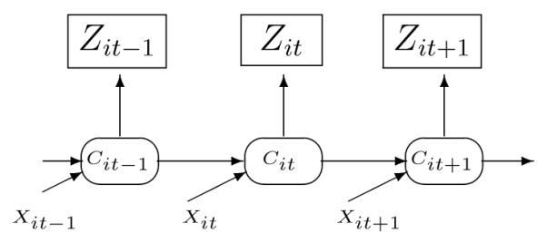
Hidden Markov model for total visits

3.2 Multiple indicator hidden Markov model

Rather than collapsing all outcomes to one total count, we propose a multiple indicator model, which simultaneously models the different encounters and links them through one shared hidden Markov chain. Since all 4 types of medical encounters come from the same individual and the exploratory analyses showed a strong association of occurrence between the different encounter types within month, we propose a multiple indicator model where the multiple outcomes Z_ijt (j = 1, 2, 3, 4) are related to a shared latent variable C_it. This multiple indicator model borrows strength across the different types of encounters to present a meaningful overall health state process for C_it that specifically captures encounters likely related to alcoholism.

Consider the following multiple indicator hidden Markov model where Z_ijt is defined as in the beginning of this section,

$$\begin{array}{cc}\hfill Z_{ijt}\mid {\theta }_{ijt}& \sim \mathit{Pois}\left(o_{jt}{\theta }_{ijt}\right)\hfill \\ \hfill \mathit{log}\left({\theta }_{ijt}\right)& ={\lambda }_{0j}+{\lambda }_{1j}{C}_{it}\hfill \\ \hfill C_{it}\mid C_{i(t-1)}& \sim \mathit{Bin}(1,\mathit{log}i{t}^{-1}({\beta }_0+{\beta }_1{C}_{i(t-1)}+\beta {\mathbf{X}}_{it}\left)\right)\hfill \\ \hfill \beta {\mathbf{X}}_{it}& ={\beta }_2{\mathrm{TRT}}_{it}^{\text{after}}+{\beta }_3{\mathrm{TRT}}_{it}^{\text{during}}+{\beta }_4{\mathbf{W}}_i\hfill \\ \hfill C_{i{t}_{i1}}& \sim \mathit{Bin}(1,{\pi }_1)\hfill \end{array}$$ (2)

This model is illustrated in Figure 2. Notice that one common health state is related to the observations of the 4 different types of medical encounters simultaneously. Specifically, it is assumed that conditional on the underlying health state, the 4 different observed counts are independent. The common health state is assumed to follow a Markov chain and the probability of transitioning to the unobserved “Unhealthy” state is determined by the health state in the previous month and other covariates. The coeffcient of ${\mathrm{TRT}}_{it}^{\text{after}}$ is again the major parameter of interest and we would expect to see a significant negative estimate for β₂ if the treatment was effective in decreasing the probability of transiting to an “Unhealthy” state as described by the 4 different types of encounters.

Figure 2.

Multiple indicator hidden Markov model

In reality, it may be that the different types of encounters do not function in exactly the same way with respect to the covariates. By assuming a shared common health state, the multiple indicator hidden Markov model is extracting that part of the 4 types of encounters which do behave similarly. If one of the types of encounters does not have any similarity with the other encounter types, this could be detected by the model since it would mean that the λ_1j associated with that encounter type would not be different from zero.

4 Model Estimation

Model estimation was done in a Bayesian framework using MCMC techniques. The joint posterior is broken into the full conditional posterior distribution with respect to each parameter and the Gibbs sampler [18] is used.

For the multiple indicator hidden Markov model, if we denote λ_j = (λ_0j, λ_1j), ${\lambda }_{\cdot }={\left\{{\lambda }_j\right\}}_{j=1}^4$, ${\beta }_{\cdot }={\left\{{\beta }_l\right\}}_{l=0}^4$, ${\pi }_{\cdot }={\left\{{\pi }_j\right\}}_{j=1}^4$, ${\mathbf{C}}_{\cdot t}={\left\{C_{it}\right\}}_{i=1}^n$, ${\mathbf{Z}}_{i\cdot t}={\left\{Z_{ijt}\right\}}_{j=1}^4$, ${\mathbf{Z}}_{i\cdot \cdot }={\left\{{\mathbf{Z}}_{i\cdot t}\right\}}_{t=t_{i_1}}^{t_{T_i}}$, ${\mathbf{Z}}_{\cdot \cdot \cdot }={\left\{{\mathbf{Z}}_{i\cdot \cdot }\right\}}_{i=1}^n$ and ${\mathbf{C}}_{\cdot \cdot }={\left\{{\mathbf{C}}_{\cdot t}\right\}}_{t=t_{i_1}}^{t_{T_i}}$, then Gibbs sampler include the following steps:

1. Give initial values for λ., β., C.., and π.

2. For the ith individual (i = 1, 2…n):

   • Sample $C_{it}^{\prime }$ from q(C_it|Z_i·t, λ., β., C_it—1, C_it+1) for t = (t_i1 + 1), (t_i1 + 2)…(t_Ti — 1)
   • Sample $C_{i{t}_{i_1}}^{\prime }$ from q(C_iti1 |Z_i·ti1, λ., β., π₁, C_{iti1 + 1}) for t = t_i1
   • Sample $C_{i{t}_{T_i}}^{\prime }$ from q(C_itTi |Z_i·tTi, λ., β., C_{itTi — 1}) for t = t_Ti where q(·|·) denotes the posterior distribution.

3. Sample λ’. from q(λ.|Z…, C..)

4. Sample β’. from q(β.|C..)

5. Take C’._t, λ’ and β’. to be the updated values and go back to step 2 until the chain converges.

The algorithm for estimation in the total visit model is just a special case of the multiple indicator model with the total visit Z_it as the outcome.

For steps 2-4, given the priors of the parameters, the full conditional posterior distribution of these parameters can be derived analytically or can be simulated by the Metropolis-Hastings Algorithm [19]. Once the chain converges, the empirical joint posterior distribution for all the parameters can be used to obtain the posterior mean and the 2.5% and 97.5% quantiles can be used as the credible interval for all the parameters.

Both the total visit model and the multiple indicator model can be implemented using WinBugs (WinBugs code given in Appendix). The priors were chosen to be as noninformative as possible. In the total visits model, flat priors were used for λ₀ and β. and Uniform(0,200) was used for λ₁.

In the multiple indicator model, because of convergence issues, the priors for λ_0j (j = 1, 2, 3, 4) and β. were strengthened to normal(0, 50) and the prior for λ_1j (j = 1, 2, 3, 4) was strengthened to uniform (0,30). The strengthened priors remain reasonable for our specific situation since e³⁰ is so big we would never expect λ_1j to go beyond 30 in reality and so is the case for λ_0j. Plus, given the fact that the sample size is so big, the information from the data is expected to dominate the parameter estimation so that it would not be very sensitive to priors.

Multiple chains with different starting values were run until convergence was achieved. Model convergence diagnosis was done by checking Gelman and Rubin statistics [20] and by visual inspection of trace plots. For a given parameter, the Gelman Rubin statistic is the ratio of the variability between parallel chains to the variability within parallel chains. The model is considered to have converged if this ratio is close to 1. Each chain was ran for 15,000 iterations with a burn in period of 5000 iterations. In fact the chains for most parameters appeared to converge much earlier than 5000 iterations (See Figures 4 and 5 for the parameters for the multiple indicator HMM) likely due to the very large sample, hence overwhelming information in the data for the parameters. The chains associated with the parameters governing the rate of Alcohol Chronic visits (i.e. λ₀₄ and λ₁₄) appeared to take longer to converge than other parameters, no doubt due to the rarity and hence very low rate of these types of encounters. Both, the multiple indicator HMM and the total visit HMM model converged with a Gelman Rubin statistics between (0.95, 1.20).

Figure 4.

MCMC iterations for the beta parameters in the mulitiple indicator HMM. Samples used for posterior estimation taken after iteration 5000.

Figure 5.

MCMC iterations for the lambda parameters in the mulitiple indicator HMM. Samples used for posterior estimation taken after iteration 5000.

In the Bayesian framework, there is technically no distinction between estimation and prediction. Hence the posterior distribution of each of the hidden states can be drawn from and saved within the MCMC sampling. Recall that the number of hidden states C_it increases with both the sample size and the number of measurements within person, and that in this data there are 395,912 (9053 individuals averaging 43.7 months of data each) different hidden states to predict. Producing and saving MCMC chains each with a few thousand iterations for each of these C_it parameters while technically possible is not computationally practical (particularly within the Winbugs software). Another way to obtain predicted values for the C_it is to use the Viterbi algorithm [21] taking the posterior mean estimates for the rest of the parameters as known. This empirical Bayes type technique commonly used for hidden Markov models produces the most likely paths for C_i. for each individual and is very fast to implement without the need to save separate MCMC chains for each state. Thus, for the purpose of comparing the predicted values from the hidden Markov models with those produced from other Poisson regression models, the Viterbi algorithm is used. The predicted underlying values for the C_it are also used to examine the appropriateness of the conditional independence assumption in the results for the multiple indicator HMM.

5 Results

5.1 Parameter estimates

Table 1 shows the results of fitting the multiple indicator HMM to the 4 different types of medical encounters per month and the results of the HMM fit to the total medical encounters per month. We see that overall the results are quite similar. In particular, both models indicate the after alcoholism treatment effect is significantly negative. The estimate of -0.07 for the after treatment effect from the multiple indicator model implies that the odds of transitioning to or remaining in the “unhealthy” state in any given month after treatment is exp(-.07) = .93 of what it was before treatment. This provides evidence in favor of the alcoholism treatment improving the health status of individuals.

Table 1.

Parameter estimates from the multiple indicator HMM, the univariate HMM for the total encounters, and the direct Poisson lagged regression model (also based on total encounters).

	Multiple Indicator HMM		Total Encounters HMM		Total Encounters Poisson regression
Parameter	mean	sd	mean	sd	mean	sd
Intercept	-3.48	0.040	-3.43	0.038	-0.23	0.029
lag 1 montha	4.59	0.026	4.59	0.026	0.13	0.009
Alcoholism Treatmentb
After Treatment	-0.07	0.018	-0.07	0.018	-0.06	0.013
During Treatment	0.36	0.030	0.33	0.029	0.25	0.026
gender(male)	-0.12	0.017	-0.12	0.017	-0.13	0.013
Age categoryc
30-39 years	0.18	0.031	0.18	0.029	0.25	0.022
40-49 years	0.24	0.031	0.24	0.029	0.31	0.022
50-59 years	0.41	0.033	0.41	0.032	0.51	0.025
≥ 60 years	0.58	0.043	0.57	0.042	0.72	0.043
Insurance Regiond
West	-0.18	0.028	-0.18	0.027	-0.26	0.022
South	-0.12	0.029	-0.10	0.027	-0.20	0.024
Northeast	-0.13	0.035	-0.13	0.033	-0.08	0.027

^alag 1 month is the previous month’s hidden state for HMM models and is the previous month’s observed count for the Poisson model.

^bbefore treatment is the reference criteria.

^c18-29 years old is the reference category

^dmidwest is the reference category.

In addition to this main finding, we see that during treatment there is a higher odds (i.e. exp(0.36)=1.43) of transitioning to or remaining in the “unhealthy” state than before treatment which matches with the expectation that during treatment individuals are actively seeking medical care. The results from the model also characterize a very strong month-to-month dependence of health state where the odds of remaining in the “unhealthy” state in the current month if an individual was in the “unhealthy” state the last month is estimated to be exp(4.59) = 98.5 times the odds of newly transitioning to the “unhealthy” state if an individual was “healthy” in the previous month.

The fact that the parameter estimates for the hidden state process from the HMM fit to the total encounters are similar to those from the multiple indicator HMM is perhaps not surprising since both models are using all the encounters (albeit in different ways). Note though that the multiple indicator model also provides specific information about how the mean encounters for each of the different encounter types are related to the underlying hidden state. The (λ_0j, λ_1j) parameter estimates from the multiple indicator HMM are: (-1.24, 3.07) for Not alcohol, (-2.42, 5.09) for Alcohol specific, (-2.00, 3.99) for Alcohol acute, and (-3.66, 6.04) for Alcohol Chronic. Furthermore, the posterior standard deviation of each λ_1j is less than 0.31 indicating that each of the encounter types is significantly related to the underlying shared health state. For example, a shift in the shared latent health state, i.e. C_it from 0 to 1 (“healthy” to “unhealthy”), will increase the mean medical encounters of Alcohol Chronic by e^6.04 times, but only increase the Non Alcohol mean medical encounters by e^3.07 times. Note that these large multiplicative increase values make sense when taken in comparison with respect to the very small background rate of encounters per person in any one month (presented in Section 2). That is, when scaled by the very small background rates of encounters, the estimated mean number of different encounter types during months indicated by “unhealhthy” states are (0.31/100)e^-3.66+6.04 = 0.03 encounters for Alcohol Chronic, (2.88/100)e^-2.00+3.99 = 0.21 encounters for Alcohol Acute, (1.25/100)e^-2.42+5.09 = 0.18 encounters for Alcohol Specific, and (20.43/100)e^-1.24+3.07 = 1.27 encounters for Not alcohol type encounters. On the other hand, when the different types of encounters are collapsed into a total encounter measure, there is only the overall estimate (λ₀, λ₁) = (-1.42, 3.28). And so the estimated mean total number of encounters during months indicated by “unhealthy” based on the HMM of the total visits is (24.88/100)e^-1.42+3.28 = 1.60 Hence the multiple indicator model is, in a certain sense, richer than the total encounters model since it provides more information.

The multiple indicator model assumes the different types of encounters are conditionally independent given the underlying hidden states. This assumption can be examined by considering the association between the encounter types after conditioning on the model predicted underlying hidden states obtained from the Viterbi algorithm. Recall from Section 2 that the simple association between occurrences of the different types of encounters were quite large particularly between the 3 different alcohol related encounters with odds ratios: 7.5 for (Alcohol Acute with Alcohol Specific), 15.8 for (Alcohol Acute with Alcohol Chronic), and 35.6 for (Alcohol Chronic with Alcohol Specific). After conditioning on the model predicted underlying hidden state, the adjusted odds ratios are dramatically decreased to 1.0, 1.8, and 3.9 respectively. Hence all or most of the association between the encounter types is explained by the hidden underlying state, though there is still some additional association particularly between (Alcohol Chronic and Alcohol Specific). This residual association indicates there may be some additional mechanism besides an underlying health state relating Alcohol Chronic and Alcohol Specific encounters. Possible extensions to the multiple indicator HMM are described in the discussion section.

5.2 Comparison with Poisson regression models

We now compare the results of the total encounter HMM and the multiple indicator HMM with two Poisson lagged regression models which are straightforward to implement in most statistical softwares; here we use SAS Proc GENMOD. For the total encounters Z_it we consider the following lagged Poisson regression model,

$$\begin{array}{cc}\hfill Z_{it}\mid {\theta }_{it}& \sim \mathit{Pois}\left(o_t{\theta }_{it}\right)\hfill \\ \hfill \mathit{log}\left({\theta }_{it}\right)& ={\alpha }_0+{\alpha }_1{Z}_{i(t-1)}+{\alpha }_2{\mathrm{TRT}}_{it}^{\text{after}}+{\alpha }_3{\mathrm{TRT}}_{it}^{\text{during}}+{\alpha }_4{\mathbf{W}}_i\hfill \end{array}$$ (3)

where o_t, ${\mathrm{TRT}}_{it}^{\text{after}}$, ${\mathrm{TRT}}_{it}^{\text{during}}$ and W_i are the same as earlier in the HMM models. This model was fit using GEE in PROC Genmod in SAS with an independent working correlation matrix and an overdispersion parameter estimated using the Pearson Chi-square. The resulting estimates and standard errors are presented in the last column of Table 1.

The coeffcient of the after treatment covariate is -0.06 with standard error 0.01 and so gives a similar result as that for the HMM although it should be noted that this estimate represents the effect on the mean number of encounters after treatment (not the effect on the odds of being in an “unhealthy” state as in the HMM). There is also a statistically significant lagged effect with previous months number of encounters being positively related to current months number of encounters estimated at 0.13 with standard error of 0.01. Altogether there are similar parameter estimates (direction and significance) found using the Poisson regression model compared to the HMM although when we examine overall fit of the Poisson lagged regression model to the fit of the HMM for total encounters we find the HMM produces a much smaller MSE: 6069 vs 8705 indicating better fit. The HMM for total encounters has two additional parameters compared to the Poisson lagged regression model, but mostly the improvement in fit is coming from the fact that the HMM does a much better job handling month to month variability in the observed encounters. Because of the strong estimated lagged effect in the Poisson regression model, if there is a high number of encounters in a particular month, the model will predict a similar high number of encounters in the next month and this has a tendency to overestimate the number of encounters when specific high values do not persist. Figure 3 compares the MSE from the two models for each individual. It is seen that for nearly all individuals, the HMM is producing better fitted values than the lagged Poisson regression model.

Figure 3.

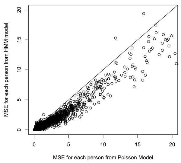
Person level Mean Square Error comparing Poisson lagged regression with HMM for Total Visits

For comparison with the multiple indicator HMM we consider the multiple source regression model [16] which also can be easily implemented in SAS Proc GENMOD. That is,

$$\begin{array}{cc}\hfill Z_{ijt}\mid {\theta }_{it}& \sim \mathit{Pois}\left(o_{jt}{\theta }_{ijt}\right)\hfill \\ \hfill \mathit{log}\left({\theta }_{ijt}\right)& ={\alpha }_0+{\alpha }_1{Z}_{ilt-1}+{\alpha }_2{Z}_{i2t-1}+{\alpha }_3{Z}_{i3t-1}+{\alpha }_4{Z}_{i4t-1}\hfill \\ \hfill & +{\alpha }_5{\mathrm{EncType}}_{ijt}+{\alpha }_6{\mathrm{TRT}}_{it}^{\text{after}}+{\alpha }_7{\mathrm{TRT}}_{it}^{\text{during}}\hfill \\ \hfill & +{\alpha }_8{\mathrm{EncType}}_{ijt}\ast {\mathrm{TRT}}_{it}^{\text{after}}+{\alpha }_9{\mathrm{EncType}}_{ijt}\ast {\mathrm{TRT}}_{it}^{\text{during}}+{\alpha }_{10}{\mathbf{W}}_i\hfill \end{array}$$ (4)

where all four different types of encounters are included and EncType_ijt is a dummy indicator specifying which type of encounter the Z_ijt is. To account for the most flexibility in lagged relationships, we allow each of the previous month’s encounter types to potentially influence each of the current month’s encounter types. The interactions between EncType_ijt and the time varying treatment covariates allow for the possibility of treatment differentially effecting different encounters. The multivariate model (4) is a very rich model and has a total of 21 parameters compared to only 17 parameters in the multiple indicator HMM. Nevertheless, the multiple indicator HMM has better fit than this Poisson regression in terms of MSE overall and for each of the separate types of encounters. Table 2 presents the resulting MSE values.

Table 2.

MSE for fit of different models. MSE is calculated as ${\sum }_{i=1}^n{\mathit{MSE}}_i$ where ${\mathit{MSE}}_i=\frac{{({\widehat{Z}}_{ijt}-Z_{ijt})}^2}{T_i}$. For the models with multiple indicators, the total MSE is just the sum of the MSE’s for each type of encounter.

	Multiple Indicators		Total Encounters
	HMM	Poisson regression	HMM	Poisson regression
Number of parameters	17	21	11	9
Total MSE	6369	10,926	6069	8705
Not Alcohol MSE	3995	8398
Alc Acute MSE	1210	1304
Alc Specific MSE	913	973
Alc Chronic MSE	251	251

6 Discussion

For the alcoholism medical utilization data, we proposed two latent variable models: a HMM for total encounters and the multiple indicator HMM for 4 different types of encounters. Both of these models assume there are unobserved health states that govern the medical care utilization of a particular person. The difference between them is that the multiple indicator model assumes that several types of medical encounters at a particular month reflect a common underlying health state, while the total visit model assumes the health state is governed only by the total frequency of encounters.

It is important to contrast the HMM models with the direct Poisson lagged regression models. The main goal of the HMM is to model changing health states over time not necessarily modeling the changing number of encounters. In the HMM, the observed medical encounters are really only a surrogate for “health status”. Measurement error (through the mixture model structure) is allowed between the observed medical encounters and the target underlying health state. For the direct Poisson models, the goal is to model the changing numbers of encounters themselves. As was seen from the examination comparing the MSE’s of the two models, the direct Poisson lagged regression model does not fit as well and particularly does not fit well when there is large month to month variability in the number of encounters. In contrast, the HMM is not as “reactionary” to large month to month variability in the number of encounters, it only models whether the values are indicative of “healthy” or “unhealthy” and the additional variability in encounters is modeled as measurement error by the Poisson distribution.

It is useful to recognize that similar models for multivariate longitudinal outcomes using a shared underlying latent variable have been considered in other situations. Focusing on describing several qualitatively distinct health states that patients can transition through, Scott et al. (2005) [22] proposed a HMM with the conditional distribution of the multivariate outcomes given the latent state following a multivariate t-distribution for data collected in a clinical trial for schizophrenia patients. Using a continuous factor analysis type framework, Roy and Lin (2000) [23] presented a model for multivariate normal longitudinal outcomes which were each hypothesized to be indicators of one underlying continuous latent variable. The longitudinal underlying latent variable was then modeled using a linear mixed effects model. These models and the multiple indicator HMM presented in the current paper take advantages of conceptualizing a latent variable underlying the multivariate longitudinal data and thus reduce the dimension of the observations while providing a succinct way of summarizing the process.

Furthermore, the multiple indicator hidden Markov model can be considered a longitudinal extension of latent class modeling. There are basically two senses in which longitudinal data have been modeled using latent class models. The first, now commonly referred to as “latent class growth modeling” [24-27] takes the vector of longitudinal measurements for each person as multiple indicators of a time-fixed latent class which essentially indicates the entire trajectory class for that individual. The other way that latent class modeling can be incorporated into longitudinal modeling is like what is being done in the current paper where there is multivariate longitudinal data i.e., doubly multivariate data. At each time point the multiple indicators are taken as measures of a time-varying latent class (hidden state) that is linked from one time to the next by the Markov property. This multiple indicator latent Markov model has been implemented specifically for ordered categorical observed data and relatively small numbers of time points via maximum likelihood [28-30]. Langeheine and van de Pol (2002) [31] give a review and description of several different Markov and latent (“hidden”) Markov models.

Several (seemingly straightforward) extensions of the HMM model presented in this paper can be considered. First, in the univariate model, the Poisson mean θ_it after adjusted for historical trend was assumed to equal e^{λ₀+λ1C_it}, with λ₀ and λ₁ fixed across individuals, however, we could instead assume that:

$$\mathit{log}\left({\theta }_{it}\right)={\lambda }_{0i}+{\lambda }_{1i}{C}_{it},\left(\begin{array}{c}\hfill {\lambda }_{0i}\hfill \\ \hfill {\lambda }_{1i}\hfill \end{array}\right)\sim N\left(\begin{array}{c}\hfill {\lambda }_0\hfill \\ \hfill {\lambda }_1\hfill \end{array},\Sigma \right)$$

thus allowing the means under “Healthy” and “Unhealthy” states for each person to be a random quantity from a bivariate normal. We could also allow a different transition probability to be fit to each person. The idea is similar to the idea of “movers and stayers” models [32-33] where some individuals may jump back and forth often from the two states while others may stay longer in the same health state due to lower probability of jumping out. In the results of the multiple indicator HMM in Section 5.1, it was pointed out that the conditional independence assumption was not satisfied entirely due to residual association between the Alcohol Specific and Alcohol Chronic encounter types. A straightforward extension to the model which weakens the conditional independence assumption is to allow covariates to be included at the measurement level, i.e., log(θ_ijt) = λ_0j + λ_1jC_it + λ_2jW_i. Finally, another possible model to consider is one that partitions time indicating treatment into more than just 3 periods (before treatment, during treatment, after treatment). Instead more complex models relating time until and time since treatment could be considered.

For future research, it is of interest to propose a practical model comparison criteria for hidden Markov models in the Bayesian framework, particularly for datasets with large sample sizes. The current Winbugs software will not produce a DIC fit statistic for finite mixture models (the HMM is a mixture model). Celeux et al. (2006) [34] discuss the problems of the usual DIC for mixture models and explore several alternative DIC’s for missing data models. In theory these DIC’s are appropriate for the HMM in the sense that the hidden states can be treated as missing data, however, in practice, the computationally most feasible one (according to [34]) among these DIC’s still encounters problems in our case. This DIC is based on conditional likelihood by considering the missing data as additional parameters. However, as was mentioned in Section 4, it is computationally infeasible to retain the MCMC samples of the 395,912 different C_it parameters in order to compute the DIC. Future work should focus on implementing relevant model fit comparisons for HMM.

Appendix

Winbugs code for total visit HMM

model { for (i in 1:Npat) {
 p[i,t_1v[i]]<-p1
 Z[i,t_1v[i]]∼dpois(theta_ot[i,t_1v[i]])
 theta_ot[i,t_1v[i]]<-Offset[t_1v[i]]*theta[i,t_1v[i]]
 theta[i,t_1v[i]]<-exp(mu[i,t_1v[i]])
 mu[i,t_1v[i]]<-lambda[1]+lambda[2]*c[i,t_1v[i]]
 c[i,t_1v[i]]∼dbin(p[i,t_1v[i]],1)
 for (t in (t_1v[i]+1):t_endv[i]){
 Z[i,t]∼dpois(theta_ot[i,t])
 theta_ot[i,t]<-Offset[t]*theta[i,t]
 theta[i,t]<-exp(mu[i,t])
 mu[i,t]<-lambda[1]+lambda[2]*c[i,t]
 c[i,t]∼dbin(p[i,t],1)
 logit(p[i,t])<-beta[1]+beta[2]*c[i,(t-1)]+beta[3]*T_a[i,t]
 +beta[4]*T_d[i,t]+beta[5]*Male[i]+beta[6]*AGE[i,t]+beta[7]*W[i,t]
 +beta[8]*S[i,t]+beta[9]*NE[i,t]
 }
 }
for (t in t_1v[person1]:t_endv[person1]) {c1[t]<-c[person1,t]}
for(t in t_1v[person2]:t_endv[person2]) {c2[t]<-c[person2,t]}
for (t in t_1v[person3]:t_endv[person3]) {c3[t]<-c[person3,t]}
lambda[1] ∼dflat() lambda[2]∼dunif(0,200) for (i in 1:9)
 { beta[i]∼dflat() }
p1 ∼dbeta(1,1)
}

Winbugs code for Multiple indicator HMM

model {
 for (i in 1:Npat)
 {
 p[i,t_1v[i]]<-p1
 c[i,t_1v[i]]∼dbin(p[i,t_1v[i]],1)
 for (j in 1:4)
 {
 Z[i,j,t_1v[i]]∼dpois(theta_ot[i,j,t_1v[i]])
 theta_ot[i,j,t_1v[i]]<-Offset[j,t_1v[i]]*theta[i,j,t_1v[i]]
 theta[i,j,t_1v[i]]<-exp(mu[i,j,t_1v[i]])
 mu[i,j,t_1v[i]]<-lambda[1,j]+lambda[2,j]*c[i,t_1v[i]]
 }
for (t in (t_1v[i]+1):t_endv[i])
 {
 c[i,t]∼dbin(p[i,t],1)
 logit(p[i,t])<-beta[1]+beta[2]*c[i,(t-1)]+beta[3]*T_a[i,t]
 +beta[4]*T_d[i,t]+beta[5]*Male[i]+beta[6]*AGE[i,t]+
 beta[7]*W[i,t]+beta[8]*S[i,t]+beta[9]*NE[i,t]
 for (j in 1:4)
 {
 Z[i,j,t]∼dpois(theta_ot[i,j,t])
 theta_ot[i,j,t]<-Offset[j,t]*theta[i,j,t]
 theta[i,j,t]<-exp(mu[i,j,t])
 mu[i,j,t]<-lambda[1,j]+lambda[2,j]*c[i,t]
 }
 }
}
for (t in t_1v[person1]:t_endv[person1]) {c1[t]<-c[person1,t]}
for (t in t_1v[person2]:t_endv[person2]) {c2[t]<-c[person2,t]}
for (t in t_1v[person3]:t_endv[person3]) {c3[t]<-c[person3,t]}
for (j in 1:4)
{ lambda[1,j] ∼ dnorm(0,0.02) lambda[2,j] ∼ dunif(0,30) }
for (i in 1:9) { beta[i] ∼ dnorm(0,0.02) }
p1 ∼dbeta(1,1)
}