Nonlinear Spectrotemporal Interactions Underlying Selectivity for Complex Sounds in Auditory Cortex

Abstract

In the auditory cortex of awake animals, a substantial number of neurons do not respond to pure tones. These neurons have historically been classified as “unresponsive” and even been speculated as being nonauditory. We discovered, however, that many of these neurons in the primary auditory cortex (A1) of awake marmoset monkeys were in fact highly selective for complex sound features. We then investigated how such selectivity might arise from the tone-tuned inputs that these neurons likely receive. We found that these non-tone responsive neurons exhibited nonlinear combination-sensitive responses that require precise spectral and temporal combinations of two tone pips. The nonlinear spectrotemporal maps derived from these neurons were correlated with their selectivity for complex acoustic features. These non-tone responsive and nonlinear neurons were commonly encountered at superficial cortical depths in A1. Our findings demonstrate how temporally and spectrally specific nonlinear integration of putative tone-tuned inputs might underlie a diverse range of high selectivity of A1 neurons in awake animals. We propose that describing A1 neurons with complex response properties in terms of tone-tuned input channels can conceptually unify a wide variety of observed neural selectivity to complex sounds into a lower dimensional description.

Introduction

Sounds such as human speech (Rosen, 1992) and monkey vocalizations (Wang, 2000; DiMattina and Wang, 2006) contain acoustic information distributed across multiple frequencies that span in time scales from a few to tens or hundreds of milliseconds. At the thalamo-recipient layers of the primary auditory cortex (A1), these sounds may be represented with high precision (Engineer et al., 2008) by neurons that are tuned to pure tones, or individual frequency components of these sounds, in a variety of species (Merzenich et al., 1975; Kilgard and Merzenich, 1999; Recanzone et al., 2000; Linden et al., 2003; Philibert et al., 2005; Moshitch et al., 2006; Sadagopan and Wang, 2008). In secondary auditory cortical areas, neurons are typically not responsive to pure tones, but exhibit tuning to complex features such as noise bandwidth (Rauschecker et al., 1995), species-specific vocalizations (Tian et al., 2001), or behaviorally relevant sounds (Hubel et al., 1959). This rapid increase in receptive field complexity led us to hypothesize that an intermediate stage might exist within A1, providing a bridge between tone-tuned thalamo-recipient A1 neurons and neurons in secondary auditory cortex that exhibit complex response properties. One likely candidate for such an intermediate stage was the population of non-tone responsive neurons that are often encountered in recordings from A1 of awake animals (Evans and Whitfield, 1964; Hromádka et al., 2008; Sadagopan and Wang, 2008). In this study, we make the first attempt to reveal underlying response properties of non-tone responsive A1 neurons in awake marmosets.

High proportions of so-called unresponsive neurons have been reported in auditory cortex of awake animals historically (Evans and Whitfield, 1964) as well as more recently (Hromádka et al., 2008), with an estimated 25–50% of neurons being unresponsive to auditory stimulation. These studies typically used relatively simple auditory stimuli such as pure tones and noise. Consistent with these results, we reported earlier that a large proportion of neurons (∼26%) in A1 of awake marmosets could not be driven using pure-tones (Sadagopan and Wang, 2008). Importantly, we found a majority of these neurons at shallow recording depths within A1. Such unresponsive or non-tone responsive neurons have been ignored by most researchers, and most reported recordings from A1 have been restricted to tone-responsive neurons, likely located in thalamo-recipient cortical layers (using reported recording depths as an indicator) in a variety of species such as primates (Recanzone et al., 2000; Philibert et al., 2005), cats (Merzenich et al., 1975; Moshitch et al., 2006), rats (Kilgard and Merzenich, 1999), and mice (Linden et al., 2003). We suspected that some of the unresponsive neurons might in fact exhibit high selectivity for particular acoustic features. In the present study, we focused on neurons recorded from superficial cortical depths of A1 that were not responsive to pure tones or even unresponsive to a wide variety of other tested stimuli.

Materials and Methods

Neurophysiology.

We recorded from A1 of three awake marmoset monkeys. Details of surgical and experimental procedures are described in a previous publication (Liang et al., 2002). All experimental procedures were in compliance with the guidelines of the National Institutes of Health and approved by the Johns Hopkins University Animal Care and Use Committee. A typical recording session lasted 4–5 h, during which an animal sat quietly in a specially adapted primate chair with its head immobilized. The experimenter monitored the behavioral state of the animal via a TV camera mounted inside the sound-proof chamber. The experimenter ensured the animal opened its eyes before stimulus sets were presented. A tungsten microelectrode (impedance 2–4 MΩ, A-M Systems) was positioned within a small craniotomy (∼1 mm diameter) using a micromanipulator (Narishige Instruments) and advanced through the dura into cortex using a hydraulic microdrive (Trent-Wells). The contact of the electrode tip with the dural surface was verified visually, which allowed us to estimate the depth of each recorded unit from the surface. We typically recorded from most well isolated single units encountered on a given track. It is quite likely that the deeper cortical layers (V and VI) were under-sampled in our experiments.

The experimenter typically advanced the electrode by ∼25 μm (in a single movement) and waited for a few minutes to allow the tissue to settle. During this period, a wide set of search stimuli was played that typically consisted of pure tones [∼5 steps per octave (oct.)], band-passed noise, linear frequency modulated (lFM) sweeps and marmoset vocalizations at multiple sound levels. This strategy of stepped electrode movements with long waits while playing a wide array of stimuli helped us detect and isolate single units with very low spontaneous activity and avoid biases toward any particular kind of units. Single-unit isolation was accomplished online using a template match algorithm (Alpha-Omega Engineering), with two additional adjustable time-amplitude windows included when necessary. Proximity to the lateral sulcus, clear tone driven responses in the middle cortical layers, tonotopic relationship with other recorded units and reversal of tonotopy at the boundaries were used to determine whether a recording location was within A1. Three of the hemispheres recorded from here overlapped with an earlier study of pure tone responses in A1 (Sadagopan and Wang, 2008), further confirming location within A1.

Acoustic stimuli.

Stimuli were generated digitally in MATLAB (MathWorks) at a sampling rate of 97.7 kHz using custom software, converted to analog signals (Tucker-Davies Technologies), power amplified (Crown Audio), attenuated (Tucker-Davies Technologies), and played from a loudspeaker (Fostex FT-28D or B&W-600S3) situated ∼1 m in front of the animal. The loudspeaker had a flat frequency response curve (±5 dB) across the range of frequencies of the stimuli used, with a calibrated level (at 1 kHz) of ∼90 dB SPL at a set level of 0 dB attenuation.

Two-pip stimuli consisted of two short 20–40 ms long tone pips, with one pip centered on an estimated best frequency (BF) to reduce search space. Since we were interested in neurons that did not respond to pure tones, estimating BF of such neurons was a difficult task. Usually, we first defined a narrow search range (usually 0.5 octaves) based on tone responses in the middle cortical layers in the neighborhood of the present electrode track. We then used a wide variety of search stimuli centered on this range including species-specific vocalizations, environmental sounds, random frequency modulated (FM) contours, amplitude modulated tones, linear and sinusoidally FM (lFM and sFM, respectively) sweeps, click trains and band-passed noise (BPN). We continued to present such complex stimuli until we elicited reliable responses to one of our search stimuli, from which we could narrow down the range of possible BFs by presenting bandpass-filtered versions of these stimuli. Determining the BF was further complicated by the fact that a majority of neurons in A1 were non-monotonically tuned for sound level [best level (BL)] with ∼25 dB widths (Sadagopan and Wang, 2008), necessitating presentation of some stimuli in our search set at multiple sound levels. On average, determining the BF and BL of a neuron on which to center our two-pip stimuli took ∼15–20 min from unit isolation. It is quite possible that we failed to drive some units because of wrong BF and BL estimates (see supplemental Discussion, available at www.jneurosci.org as supplemental material). We typically presented five repetitions of any given stimulus (tones, vocalizations, etc.) and used a Wilcoxon rank sum test at p < 0.05 to establish whether a given neuron was significantly driven by that stimulus, compared with spontaneous rate of the neuron over the entire stimulus set.

Once BF and BL of a unit were determined, we fixed the frequency of one pip at BF and changed the frequency and onset time of the second pip with respect to the BF pip (Figure S1A, available at www.jneurosci.org as supplemental material). We usually sampled ± 1 octave in frequency (1/8 octave bins) and ± 100 ms in time (12.5 ms bins). Stimuli were presented in a randomized manner and each two-pip combination was repeated at least eight times. We also presented single-pip stimuli of the same length to estimate single-frequency contributions to the response. On average, it took ∼40 min to complete a typical two-pip stimulus set. Taken together with the time to estimate BF, arriving at the nonlinear response map took ∼1 h of recording time from single unit isolation. We completed presentation of eight repetitions of the entire two-pip stimulus set (typically, n = 289 stimuli) on 118 neurons with maximal tone response <22 spikes/s. We chose this cutoff based on an earlier study from our laboratory in the same preparation that observed a median tone driven response at BF of 22 spikes/s for a population of sharply tuned tone-responsive units. Forty-one of 118 neurons showed statistically significant supralinear excitatory responses (p < 0.05 compared with sum of individual pip responses, modified permutation test, see below) to at least one two-pip combination. Twenty-two of these 41 neurons (54%) were completely unresponsive to pure tones. We collected responses of neurons to other stimuli such as lFM sweeps, click trains and vocalizations that overlay the two-pip interaction map to determine whether these responses could be explained by the two-pip interaction map (typically 3–5 repetitions). However, this step was constrained by unit isolation quality, as median hold time for single units in our preparation was ∼50 min.

Analysis and statistics.

To quantify the degree of nonlinearity we used the following framework: R(spikes/s) = a_f0 + b_Δf + c_{f0*Δf;Δt}, %Nonlinearity = c/(a + b) * 100. Here, R was the neuron's response to the combination of two tone pips, a was the response to the BF pip alone, and b was the response to the second pip alone. These quantities were measured experimentally by presenting the combination stimuli and single tone pips. We calculated c, the purely interactive term arising from the combination of frequencies (f0 and Δf) at a particular relative onset time (Δt), from the above equation. We then determined the ratio of the second-order term to the sum of first-order terms as a measure of nonlinearity. To prevent this ratio from artificially inflating due to zero tone responses, we did not subtract out spontaneous spikes from our estimates of a − c. Therefore, the %Nonlinearity measure should be treated as a lower bound. Nonlinear maps plotted in figures are the purely second-order component given by c. These maps were smoothed for visualization purposes only. Statistical significance was established by comparing each combination's response distribution with the average value of a + b using a t test (as a prefiltering step) and with all possible permutations of a + b values (usually 64 values resulting from 8 repetitions each of a and b) using a Wilcoxon rank-sum test (resulting in a modified permutation test). In 41 neurons, we obtained p < 0.05. In 39 of these cases, we obtained p < 0.01. It could be argued that we are designating a given neuron as “nonlinear” or not based on multiple independent statistical tests (one for each combination response bin). Therefore, we also required that the p value in at least the bin with maximal response (peak p-value) also met multiple-comparison corrected criteria. All 39 neurons with uncorrected peak p < 0.01 met Bonferroni-corrected criteria as well (actual p value <1.7 × 10⁻⁴ for a typical stimulus set consisting of 289 stimuli). These neurons were used for final population analysis (histogram of actual peak p values from all neurons is shown in Fig. 7D).

Figure 7.

Generality and robustness of A1 nonlinear neurons. A, We did not find any differences in the distributions of BFs (top) or BLs (bottom) between nonlinear neurons (black histograms) and tone-responsive neurons (gray histograms) suggesting that the observed phenomenon was a general computation (n.s., not significant). B, High nonlinearity observed was not a consequence of using short stimuli to obtain linear response rates. When responses to 100-ms-long pure tones were used to compute single-tone response rates, we still observed significant nonlinear facilitation when compared with two-pip responses computed using 20–40 ms pips. The neuron falling below the diagonal (y = x line) presumably exhibited a stimulus length effect. C, Predicted versus actual preferred lFM velocities of a subset of nonlinear units (n = 22; **p < 0.01). Inset, Predicted versus actual preferred BWs of BPN stimuli in another subset of nonlinear units (n = 8; not significant). D, Distribution of actual p values from all neurons that met our initial screening criterion of peak p < 0.05, modified permutation test (n = 41, gray histogram). Dotted line indicates the Bonferroni-corrected p value criterion for the most common stimulus set (n = 289 stimuli). Thirty-nine of 41 neurons met this criterion.

To quantify selectivity and population sparseness of neural populations (pure-tone and nonlinear), we measured reduced kurtosis of the firing rate distributions obtained in response to a given stimulus set (Lehky et al., 2005; Sadagopan and Wang, 2008). Briefly, if a neuron responded well to all stimuli in a given set, the firing rate distribution would be symmetric about the mean with low kurtosis. However, if a neuron only responded to a few stimuli in a given set (highly selective responses), the resultant firing rate distribution would be asymmetric with high kurtosis. Similarly, population sparseness could be derived by constructing firing rate distributions of a population of neurons responding to a given stimulus.

Results

We recorded from a total of 460 well isolated single-units located in A1 from three awake marmoset monkeys. Most of these units (342/460, 74%) exhibited significant pure-tone responses and their response properties have been described in an earlier study (Sadagopan and Wang, 2008). However, out of the total population of 460 units, 118 units did not significantly respond to pure tones (∼26% of total sample). In this study, we focused attention on these 118 seemingly unresponsive neurons. We discovered that these neurons responded with significant firing rates to at least one of the following complex stimuli: lFM sweeps, sinusoidally amplitude modulated (sAM) tones, narrowband click trains, BPN, two-pip stimuli, marmoset vocalizations, or environmental sounds. These 118 unresponsive units were studied with the two-pip stimulus set. Forty-one of the 118 units (35%) showed statistically significant nonlinear interactions in their two-pip responses (see Materials and Methods). We will first present representative single-unit examples in detail to illustrate the diversity of responses that we observed among non-tone responsive neurons in A1 of awake marmosets. We will then present population analyses of these non-tone responsive neurons.

Complex feature selectivity of A1 neurons and underlying nonlinear interactions

In superficial cortical depths of A1 in awake marmosets, we often encountered neurons that exhibited high stimulus selectivity to particular features of complex sounds such as marmoset vocalizations. Figure 1A illustrates the responses of one such example neuron [significant responses to 6 of 40 vocalization tokens consisting of 20 natural (forward) calls and their reversed versions]. Figure 1B shows the spike responses of this unit to the particular vocalization (a trill-twitter) that elicited the maximal response overlaid on the vocalization spectrogram with spikes plotted around the BF of this neuron (6.9 kHz). In addition to preferring the natural to the reversed vocalization (Wang et al., 1995; Wang and Kadia, 2001), we made the qualitative observation that this unit reliably responded only when a particular feature (upward FM “trill” element) of the natural call occurred. Despite its location within A1, this unit was unresponsive to tones (Fig. 1E).

Figure 1.

Selectivity for complex features in A1. A, Raster of example neuron's responses to marmoset vocalizations (n, “natural”; r, “reversed”). Gray shading corresponds to stimulus duration; different vocalization tokens had different lengths. Gray and black dots correspond to spontaneous spikes and spikes falling within our analysis window (15 ms after stimulus onset to 50 ms after stimulus offset) respectively. B, Responses to a particular token (“trill-twitter” call and reversed version) showed preference for natural over reversed call. Also note that maximal response occurs immediately following the initial upward-going trill segment. C, This unit responded strongly to a specific combination of two tone pips—a 5.8 kHz pip followed 75 ms later by a 6.9 kHz BF pip (red disk, both pips at 20 dB SPL). Purely second-order interaction map is plotted; image is smoothed for display. Colormap indicates the percentage of facilitation over sum of first-order responses (see Materials and Methods), and dark red contour and pink contour denote significance at p < 0.01 and p < 0.05 (modified permutation test) respectively. The nonlinear component was 180% of the sum of linear components (number in corner of interaction map). Gray lines are diagrams of lFM sweep stimuli tested in D; intensity corresponds to response strength (lightest = 0 spikes/s, darkest = 12.5 spikes/s; u, upward; d, downward lFM sweep direction). D, This unit strongly responded to “up” FM sweeps that connected the RF subunits in the nonlinear map and not to “down” FM sweeps that spanned the same frequency range (mean ± 1 SD plotted). The unit was tuned to an 80-ms-long upward lFM sweep spanning 5.6 kHz to 7.2 kHz (darkest gray line in C), precisely connecting the subunits. E, This unit was unresponsive to pure tones over a wide range of frequencies (2 octaves) and levels around estimated BF and BL (raster shown; frequency and level are interleaved on y-axis).

However, the kind of data shown in Figure 1A by themselves do not reveal what causes such high stimulus selectivity. We hypothesized that precise nonlinear spectrotemporal integration of tone inputs could generate the RF complexity underlying the high stimulus selectivity we observed. To determine these putative nonlinear interactions, we developed a two-pip stimulus set (Fig. S1A, available at www.jneurosci.org as supplemental material; see Materials and Methods for details). Based on responses to these stimuli, we constructed nonlinear (second-order) “two-pip interaction maps” that revealed how discrete tone-tuned subunits interacted over frequency and time to result in each neuron's response.

The two-pip interaction map for the neuron shown in Figure 1 revealed that the minimal effective stimulus for this neuron was the combination of a 5.8 kHz pip followed 75 ms later by a 6.9 kHz BF pip, with both pips at 20 dB SPL (Fig. 1C). When we tested this neuron with upward and downward linear FM sweeps spanning a range of frequencies from 5.6 to 7.2 kHz (0.363 octave span ∼6.9 kHz; gray lines overlaid on Fig. 1C), it showed tuning for the 80-ms-long upward sweep (Fig. 1D), as would be predicted from the two-pip interaction map in Figure 1C. The exquisite sharpness of this neuron's tuning to this feature should be emphasized; at half-maximal response, the unit responds to FM sweep velocities ranging from 3.63 oct./s (16 Hz/ms) to 6.04 oct./s (26.7 Hz/ms).

The two-pip interaction map (Fig. 1C) also explains this neuron's responses to vocalizations (Fig. 1A,B). Qualitatively, one can observe that the initial upward-going trill part of the vocalization in Figure 1B is an ∼100 ms long upward frequency modulated fragment ∼6 kHz that overlays the subunits of the two-pip interaction map shown in Figure 1C. However, in the reversed version of this vocalization, the upward frequency modulated fragment becomes downward and no longer overlays the subunits of the two-pip interaction map. As shown in Figure 1B, this neuron did not respond to the reversed vocalization. These response examples illustrate how this neuron's selectivity to FM sweep “fragments” and preference for forward over reversed calls are related response properties, and how they arise from a simple underlying nonlinear computation.

Figures 2–4 show further single-unit examples of such complex tuning properties observed in non-tone responsive neurons in A1. The unit in Figure 2A–D was unresponsive to tones but responded robustly and was tuned without stimulus synchronization to interclick intervals of 40 and 80 ms (Fig. 2B, left, C) of a Gaussian pulse train stimulus set (tonal click-trains at BF with Gaussian envelopes, SD = 8 ms) with varying interclick intervals. We also found that this neuron could be driven more strongly by a train of 50 ms long upward lFM sweeps centered ∼8.5 kHz and repeating every 50 ms (Fig. 2B right, D), but required at least 2 repeated linear FM sweeps to elicit a response. Detecting repetitive FM sweeps is relevant to tasks such as vocalization recognition (for example, of marmoset twitter calls). On deriving its two-pip interaction map, we discovered subunits at BF representing a repetitive temporal structure of a ∼40 ms repetition period (Fig. 2A; labeled “1” and “2”), with an additional subunit occurring at a lower frequency and earlier time than the BF subunit (Fig. 2A; labeled “3”). This nonlinear RF structure could explain the neuron's preference for the particular interclick intervals, FM sweep repetition periods, direction and the minimum number of sweeps we observed. Spike rasters of pulse train and lFM responses are displayed in Figure 2B to demonstrate robustness of response.

Figure 2.

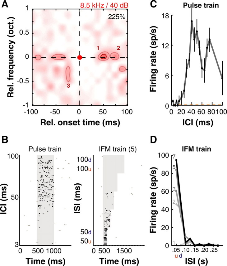
Example A1 neuron that displayed selectivity to repetitive stimuli. A, Subunits were observed at 8.5 kHz (BF) spaced at ∼50 ms intervals. Another significant subunit was located 0.25 octaves below BF occurring ∼25 ms earlier. B, Spike rasters of this neuron's response to Gaussian pulse trains (left) and lFM sweep trains (right) (5 sweeps per train). Responses were sustained throughout stimulus duration. C, Consistent with the nonlinear response map, this unit was tuned to interclick intervals of 40 and 80 ms when tested with Gaussian pulse train stimuli at BF (carrier frequency 8.5 kHz, click width SD 4 ms; mean ± 1 SD plotted). ICI, Interclick interval. D, The unit preferred 50-ms-long upward lFM sweeps trains ∼8.5 kHz with a preferred intersweep interval of 50 ms, also consistent with A. At least two sweeps were required to elicit a response. Darkest line corresponds to 7 sweeps in train, lightest line to a single sweep. ISI, Intersweep interval. Colormap, contours and raster conventions as in Figure 1. “u” and “d” refer to upward and downward lFM sweeps and are alternated along the axis.

Figure 3.

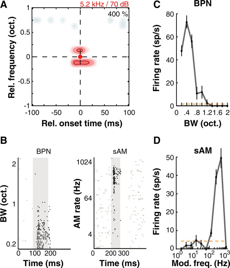
Example A1 neuron showing purely spectral combination sensitivity. A, Nonlinear interaction map for this neuron showed excitatory subunits located 1/8 oct. above and below BF at coincident onset times with the BF pip. B, Spike rasters of this neuron's response to BPN of different BWs (left) and sAM at different modulation rates (AM rate; right). C, This unit was tuned to a bandwidth of ∼0.4 oct. centered at BF and BL, consistent with the nonlinear map obtained. D, Interestingly, this unit was narrowly tuned to sAM tones at 5.2 kHz modulated at 512 Hz. It should be noted that at a BF of 5.2 kHz, this amplitude modulation at 512 Hz produces spectral sidebands that are ∼1/8 oct. away from BF. Thus, these responses are also consistent with the nonlinear map in A. Error bars correspond to ± 1 SEM; dashed orange line is spontaneous rate. Colormap, Contours and raster conventions as in Figure 1.

Figure 4.

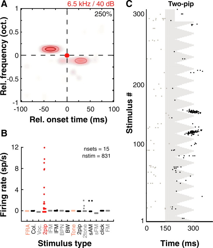
Nonlinear spectrotemporal interactions underlie complex feature selectivity in A1. A, Nonlinear interaction map of another example A1 neuron that showed strong nonlinear interactions around a BF of 6.5 kHz. B, However, this unit did not respond to a wide variety of commonly used stimuli. Red circles are responses to two-pip stimuli and pink circles are responses to pure tones. Each dot is driven response rate (after subtracting spontaneous rate) to an individual stimulus belonging to that particular stimulus set. Abbreviations used in addition to those defined in text are as follows: FRA, frequency response area (tones); Col., colony noise (environmental sounds from monkey colony); Voc., marmoset vocalizations, BW − BPN of varying bandwidths. C, Raster of two-pip responses corresponding to map in A showing robust spiking occurred after integration of both pips. Colormap, Contours and raster conventions as in Figure 1.

Figure 3 shows an example of selective stimulus tuning and underlying nonlinear interactions along the spectral dimension. This neuron was unresponsive to pure tones, but tuned to band-passed noise centered at 5.2 kHz with a 0.4 octave bandwidth presented at 70 dB SPL (Fig. 3B, left, C). This neuron was also tuned to a specific modulation frequency (512 Hz) of sAM tones with a center frequency of 5.2 kHz presented at 70 dB SPL (Fig. 3B, right, D). In a stimulus-based description framework, this neuron would be described as one that was tuned to the bandwidth of band-passed noise, such as those reported earlier in the lateral belt (LB) of macaque monkeys (Rauschecker et al., 1995), or one that had a certain rate-based modulation transfer function (rMTF), similar to earlier descriptions of A1 neurons (Liang et al., 2002). However, from the two-pip map in Figure 3A, it is clear that both the noise and sAM responses are generated by a simple underlying computation. In this case, the two-pip map exhibited excitatory “side bands” that were located 0.125 oct. away from BF at both higher and lower frequencies occurring simultaneously with the BF pip. Band-passed noise excited both these second-order peaks in addition to the BF peak causing a response. It should be noted that at a BF of 5.2 kHz, amplitude modulation of 512 Hz created side-bands that were ∼0.125 oct. distant from the 5.2 kHz spectral peak. Therefore, the peak of the rMTF of this neuron appeared to be caused by a spectral, rather than temporal effect of amplitude modulation.

The neuron in Figure 4A–C is a more complex example. While we successfully obtained a two-pip interaction map for this unit (Fig. 4A), we could not drive this unit using any other stimuli from an extensive repertoire. Figure 4B plots the firing rates of this neuron to 831 stimuli of 15 different types, including species-specific marmoset vocalizations, environmental sounds, lFM sweeps, random FM contours, sAM tones, noise of different bandwidths and click trains. Only a few two-pip stimuli (40 ms pips) elicited significant responses. Some of the FM stimuli used in the testing included those that “connected” the nonlinear peaks in the two-pip interaction map (similar to stimuli in Fig. 1C) but did not elicit any response. Therefore, this neuron seemed to prefer discrete pips that occurred immediately in succession. This neuron's responses to the preferred two-pip stimuli were strong, robust and occurred after both pips (Fig. 4C), as would be expected from a computation that integrates multiple inputs over time.

Over the four single neuron examples discussed above, we observed some of the most representative stimulus tunings found in neurons located in superficial cortical depths within A1, which included (but was not limited to) sharp tuning to FM sweep velocity, selectivity to vocalizations, non-synchronized bandpass tuning to click rate, tuning to repetition rates of FM sweep trains, tuning to sAM frequency, tuning to bandwidth of band-passed noise, selectivity for features of environmental sounds and selectivity for discrete tone-pip combinations. This heterogeneity was typical of the population of non-tone responsive neurons that we recorded from.

Population response properties

Here we report population analysis based on 39 of 41 nonlinear neurons that passed the more stringent Bonferroni-corrected statistical criteria (see Materials and Methods). Despite the heterogeneity of individual non-tone responsive neurons, several consistent features were evident across the sampled population with respect to their two-pip response maps. First, these neurons were not responsive or only weakly responsive to pure-tone stimulation. Twenty-two of 41 (54%) neurons were completely unresponsive pure tones, and median pure-tone response of the remaining 19 neurons was 16 spikes/s (Fig. 5A, gray histogram). Using two-pip stimuli, however, we were able to drive these neurons significantly above their pure-tone responses (Fig. 5A, median peak driven rate of two-pips: 24 spikes/s; range: 16 spikes/s to 86 spikes/s; black histogram). On average, we observed a 250% nonlinearity as a result of the spectrotemporal interaction of two-tone pips (Fig. 5B). Histograms of spectral and temporal precision of the second-order subunits (extents of subunits at 50% maximum facilitation) are plotted in Figure 5C. The observed second-order peaks were precise to the order of 0.125 oct. in frequency and 12.5 ms in time. Such high precision in frequency was consistent with the tuning widths observed in a population of level-tuned pure-tone responsive neurons in A1 that may form the putative inputs to nonlinear neurons (median 0.25 oct.) (Sadagopan and Wang, 2008).

Figure 5.

Response enhancement by two-pip stimuli in nonlinear A1 neurons. A, Nonlinear neurons were not responsive to tones (median = 0 spikes/s, gray histogram). However, using two-pip stimuli, we could drive these neurons to a median of 24 spikes/s (black histogram), comparable to the median pure tone response (at BF) of tone-responsive neurons in the awake marmoset. (**p < 0.01; Wilcoxon rank-sum test). B, When we quantified degree of nonlinearity (see Materials and Methods), we observed a median 250% facilitation over the sum of linear components. C, Histograms of precision in frequency and time of the second-order subunits (half-maximal extent). Median spectral and temporal precision were 0.125 oct. and 12.5 ms respectively.

It is important to note that although the actual duration in which stimulus energy was present was only 2*pip-length, the estimated firing rates for two-pip stimuli were calculated within a window stretching from the onset of the first pip to 50 ms after the offset of the second pip (minimum window length of 70 ms and maximum window length of 230 ms in our entire data set). We used this conservative metric because in the context of feature selectivity, the delay between the two pips might be viewed as an essential part of the “stimulus,” as neural response is contingent upon this delay. Therefore, the reported maximum firing rates for two-pip stimuli could be underestimates. In terms of the absolute number of spikes elicited, a median response rate of 24 spikes/s translates to 1.7 spikes/trial for the shortest (70 ms) stimuli and 5.5 spikes/trial for the longest (230 ms) stimuli in our stimulus set. In comparison, for a population of finely tuned tone-responsive units at a median response rate of 22 spikes/s (Sadagopan and Wang, 2008), 2.2 spikes/trial were elicited for 100 ms pure-tone stimuli. Therefore, the nonlinear neurons were driven as robustly as tone-tuned neurons given the right stimuli.

Second, these neurons were commonly found in superficial cortical depths as evidenced by both absolute (from dural surface) and relative (from first neuron encountered) recording depth measurements (black dots, Fig. 6A). In contrast, the tone-responsive neurons were more commonly found at deeper cortical depths (gray dots, Fig. 6A). The nonlinear neurons exhibited a significantly lower (p < 0.01; Wilcoxon rank-sum test) median spontaneous rate (0.9 spikes/s) than pure-tone responsive neurons (2.7 spikes/s), suggesting that they are likely to be “missed” if only spontaneous spikes or simple acoustic stimuli are used to “search” for these neurons. Most subunit frequencies in the two-pip interaction maps were <0.5 octaves from BF (Fig. 6B), which corresponds to a <500 μm distance on the cortical surface of the marmoset (Aitkin et al., 1986). Temporal interactions were also over short time scales (mostly <50 ms, Fig. 6B). These data thus suggest a highly localized computation, possibly occurring at a columnar scale.

Figure 6.

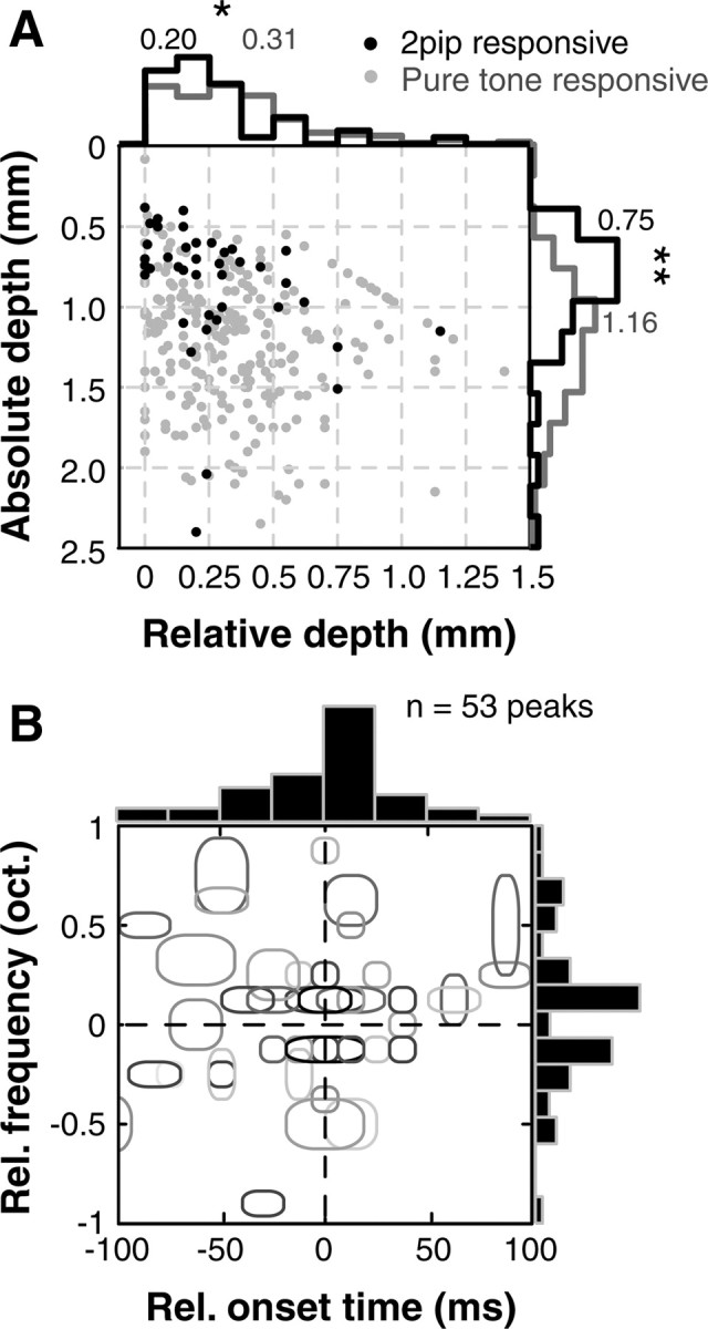
Location and properties of nonlinear neurons in A1. A, Distribution of absolute depth (from dural surface) and relative depth (from first neuron encountered) of nonlinear (black dots) and tone-responsive (gray dots) units. Nonlinear units were located at shallower cortical depths compared with tone-responsive units (histograms of absolute and relative depths are on margins, numbers are medians; *p < 0.05, **p < 0.01, Wilcoxon rank-sum test). This suggested that nonlinear neurons may be localized to superficial cortical layers. B, Distribution of all observed subunits plotted relative to normalized BF. Gray ellipses are locations of statistically significant nonlinear subunits; shading corresponds to the percentage of facilitation. Most subunits were located <0.5 octaves away from BF suggesting a local computation. Most subunits also occurred within 50 ms of the BF pip.

Third, the observed nonlinear interaction exhibited generality across the frequency and sound level dimensions. The distribution of the BF estimated for the nonlinear neurons was indistinguishable from the BF distribution obtained from 275 pure-tone responsive neurons (Fig. 7A, top). Similarly, the distribution of BLs for the nonlinear neurons was also no different from the distribution of BLs of pure-tone responsive neurons observed (Fig. 7A, bottom). These data also suggest that a common mechanism might underlie the generation of such nonlinear units over a wide range of frequencies and sound levels.

The observed degree of nonlinearity was not a consequence of using short tone-pips (20–40 ms) for estimating first-order response strengths or an overall stimulus length/energy effect for the following reasons. In only 1 of 39 cases, we observed no facilitation when comparing interaction responses using short pips (20–40 ms) to single tone responses using longer stimuli (100 ms). This neuron responded to pure tones, but only of longer lengths. In all other cases, a high degree of supralinear facilitation occurred even when compared with long (100 ms) pure tones (Fig. 7B). This suggests that the observed nonlinear facilitation effect was not a consequence of using short tone-pips that resulted in artificially low estimates of the first order responses. Moreover, an overall energy effect was ruled out due to the fact that most of the nonlinear neurons were non-monotonically tuned to sound level (distribution of BLs shown in Fig. 7A). An increase in the sound level stimuli typically resulted in the cessation of responses, an observation inconsistent with energy integration models. It should be noted that the putative tone-tuned inputs to these nonlinear units are also tuned to sound level (Sadagopan and Wang, 2008).

To assess how well the relative positioning of subunits in a given nonlinear interaction map could predict a neuron's responses to complex stimuli, we compared predictions of preferred lFM velocities derived from nonlinear interaction maps to actual lFM velocity tuning curves obtained by presenting lFM stimuli in a subset of neurons (n = 22). The nonlinear interaction maps of these neurons exhibited subunits that were separated in both frequency and time (nonzero Δf and Δt), suggesting that these neurons could be selective to FM sweeps. The predicted “preferred” lFM velocity of each neuron was simply taken as the slope of the line connecting the peaks of the subunits (Δf/Δt) without interpolation, expressed in octaves/s. The actual preferred lFM velocity was the lFM velocity that generated the maximum firing rate in a neuron. Because the parametric lFM stimuli used were typically centered on the BFs of the nonlinear neurons, firing rates were calculated in an analysis window beginning 15 ms after stimulus onset and ending 50 ms after the IFM sweep crossed the BF in the case of upward sweeps, or beginning 15 ms after BF crossing and ending 50 ms after stimulus offset for downward sweeps. From the plot of predicted versus actual velocity selectivity (Fig. 7C), it is evident that the nonlinear map robustly predicts the lFM velocity selectivity (r² = 0.574; p < 0.01). Note that because these neurons do not respond to pure-tones, it is not possible to predict a preferred lFM velocity using pure-tone responses alone. In a smaller subset of neurons where subunits were separated in frequency alone (Δt = 0, n = 8), we attempted to predict the preferred bandwidth (BW) of BPN stimuli (predicted BW = Δf + 2*subunit halfwidth). In this case, predictions were markedly poorer (Fig. 7C, inset; r² = 0.39; p = 0.06), perhaps because inhibitory subregions could not be adequately uncovered by the two-pip stimulus set (see Discussion).

Functional differences between pure-tone and nonlinear neurons

Functionally, the representation of complex sounds by the population of pure-tone and nonlinear neurons may be quite different. For example, Figures 8, A and B, are spike rasters of a pure-tone neuron (BF = 8.6 kHz) and a nonlinear neuron in response to a stimulus set consisting of 20 marmoset vocalizations and their reversed versions. An additional example of a nonlinear neuron's responses to the same set of vocalization stimuli is shown in Figure 1A. Pure-tone neurons typically respond when components in a vocalization cross the neuron's BF, resulting in responses to many features present in many vocalization tokens. In contrast, nonlinear neurons exhibit far greater selectivity to vocalization stimuli, responding only when particular features in a small number of vocalizations are present. This leads to much more selective responses to vocalization stimuli, as evident from the spike rasters (Figs. 1A, 8B). Figure 8, C and D, show distributions of the firing rates of the data shown in Figure 8, A and B, respectively, calculated over the entire duration of each vocalization stimulus after subtracting spontaneous firing rate. The exemplar tone-tuned neuron (Fig. 8A,C) responded with a mean firing rate of 5.9 ± 5.15 spikes/s to 40 stimulus tokens, with most stimuli eliciting similar firing rates. This resulted in a largely symmetric distribution with low kurtosis about the mean (κ = 0.185; see Materials and Methods) (Lehky et al., 2005). The exemplar nonlinear neuron (Fig. 8B,D) however, failed to respond to most stimuli (mean firing rate = 0.65 ± 1.33 spikes/s), and elicited large responses for only few stimuli from the entire set. Consequently, the firing rate distribution for this neuron exhibited high kurtosis (κ = 14.22). Over the population, pure-tone neurons were almost three times as responsive to the 40 vocalization stimuli (population mean firing rate = 4.6 ± 9.2 spikes/s, n = 35) compared with the nonlinear neurons (population mean firing rate = 1.6 ± 3.8 spikes/s, n = 22). Pure-tone neurons were also driven to a higher peak firing rate (mean = 46.5 ± 45.2 spikes/s, calculated in 20 ms bins, spontaneous rate subtracted) than nonlinear neurons (mean = 24.6 ± 25.5 spikes/s), averaged over the entire vocalization stimulus set.

Figure 8.

Differential representation of vocalizations in pure-tone and nonlinear neuron populations. A, Spike raster of an example pure-tone neuron responding to 20 natural marmoset vocalizations (n) and their reversed versions (r). Gray shading is stimulus duration, black dots are spikes falling within analysis window, gray dots are spontaneous spikes. B, Same as A, but for an example nonlinear neuron. C, Distribution of firing rates obtained from the raster in A for the pure-tone neuron. D, Same as C, but for nonlinear neurons. κ denotes the excess kurtosis of the distributions. E, Distributions of selectivity for nonlinear (black) and pure-tone (gray) neurons. Nonlinear neurons exhibited more selective responses than pure-tone neurons (*p < 0.05, Kolmogorov–Smirnov test). F, Distributions of population sparseness for nonlinear (black) and pure-tone (gray) neurons. Nonlinear neurons represented complex stimuli more sparsely than pure-tone neurons (**p < 0.01, Kolmogorov–Smirnov test).

We used the excess kurtosis of the firing rate distributions to quantify the selectivity and population sparseness of pure-tone and nonlinear neurons (see Materials and Methods) (Lehky et al., 2005; Sadagopan and Wang, 2008). Because such analyses require that identical stimuli be presented to all constituent neurons, we performed it only on 22 nonlinear neurons and 35 pure-tone neurons that were presented with the same vocalization stimulus set (20 forward marmoset calls and their reversed versions). Because these neurons had different BLs, the only difference was the sound levels at which the stimulus sets were presented. All neurons included in this analysis exhibited significant responses (p < 0.05, t test compared with spontaneous rate) in at least one 20 ms bin to at least one of the stimuli. Note that the accuracy of such analyses is constrained by the number of neurons and stimuli used. Figure 8, E and F, are comparisons of the selectivity and population sparseness of pure-tone (gray) and nonlinear neurons (black) respectively. Nonlinear neurons showed significantly higher selectivity for vocalization stimuli (pure-tone neuron median = 2.4, nonlinear neuron median = 4.8; p < 0.05, Kolmogorov–Smirnov test) and higher population sparseness (pure-tone neuron median = 2.6, nonlinear neuron median = 7.5; p < 0.01, Kolmogorov–Smirnov test) than pure-tone neurons. Therefore, a given nonlinear neuron responded to fewer stimuli in a stimulus set (i.e., higher selectivity), and fewer nonlinear neurons of the population responded to a given stimulus (i.e., higher population sparseness) compared with pure-tone neurons. This highlights the transformation in the representation of complex stimuli that occur between populations of pure-tone and nonlinear neurons.

Discussion

Combination-selectivity of non-tone responsive neurons in A1 of awake marmosets

A high proportion of apparently unresponsive neurons (25–50%) have been reported by previous studies in awake animals (Evans and Whitfield, 1964; Hromádka et al., 2008; Sadagopan and Wang, 2008). These neurons have not been systematically studied, and it has been unclear what function they might serve. Our findings demonstrate that non-tone responsive neurons are in fact nonlinear and highly selective for complex stimuli. The broad distributions of BF and preferred sound level of nonlinear neurons suggest that they may serve as “feature detectors” for a wide range of complex sounds such as marmoset vocalizations. It should be emphasized that the high selectivity, non-tone responsiveness and low spontaneous firing rates of these neurons make them difficult to isolate and drive, which may explain why earlier studies have not encountered a large number of such neurons. Three methodological factors helped us successfully accomplish our experiments: (1) the use of a rich and complex stimulus set consisting of both natural and artificial stimuli, (2) interactively determining stimuli that best drive each neuron based on their responses to these stimuli, rather than using a “standard” stimulus set, and (3) the use of a stop-and-search strategy while searching for units (see Materials and Methods).

Nonlinear neurons were located at superficial cortical depths as measured by absolute and relative electrode depth measurements, but we did not confirm their laminar location using anatomical tracing methods. The clear differential distributions of both absolute and relative depths of nonlinear and tone-responsive neurons (Fig. 6A) offered strong evidence that the nonlinear neurons were located in superficial cortical layers (layers II/III), and may be at a higher stage of an auditory processing hierarchy than pure-tone responsive neurons. The low spontaneous rates of these neurons may offer further support for a superficial laminar location. However, it is possible that some of these neurons might be located in the thalamo-recipient layers. It is also likely that the deep (infragranular) cortical layers were undersampled in our experiments.

Relationship to earlier studies

Combination-sensitive responses have been well described in the auditory system of echolocating bats at both cortical and subcortical levels (Suga et al., 1978, 1983; O'Neill and Suga, 1979; Suga, 1992; Esser et al., 1997; Razak and Fuzessery, 2008). Combination-sensitive neurons that are specific to song sequences have been observed in songbirds (Margoliash, 1983; Lewicki and Konishi, 1995). Our findings from awake marmosets support the notion that the combination-selectivity initially demonstrated in echolocating bats is a general organizational principle for cortical neurons across many species. Our data differ from these previous studies in that we show a much greater diversity of best frequencies, best levels, frequency differences, and longer time scales of combination-selectivity (of the order of an octave in frequency and tens of milliseconds in time), as opposed to several kilohertz and a few milliseconds, distributed within the range of echolocation frequencies and levels in bats (Suga et al., 1978, 1983; O'Neill and Suga, 1979).

Spectrotemporal interactions of many different flavors have also been described in pure tone-responsive neurons of primary auditory cortex in nonspecialized systems (Nelken et al., 1994a,b; Brosch and Schreiner, 1997, 2000, 2008). Linear spectrotemporal interactions between frequency channels have been observed in tone-responsive A1 neurons using STRF estimation methods (deCharms et al., 1998; Miller et al., 2002; Depireux et al., 2001). Other nonlinearities such as those with respect to stimulus contrast (Barbour and Wang, 2003), sound level and adaptation (Ahrens et al., 2008) and foreground-background interactions (Bar-Yosef et al., 2002) have also been reported in tone-responsive neurons in A1. Of particular note is the study of awake owl monkey A1 by deCharms et al. (1998) that demonstrated how stimuli that matched a given neuron's linear STRF elicited stronger responses than nonmatched stimuli, and in some cases could predict a neuron's selectivity to certain stimulus features. In the present study, we made a similar observation but with an important difference—we specifically investigated the nonresponsive and putatively nonlinear neurons in awake marmoset A1. For these neurons, stimuli overlying their nonlinear receptive fields in frequency and time elicited maximal responses, and the nonlinear interaction map could predict these neurons' responses to some complex sounds.

Methods to study nonlinear neurons

We did not use reverse correlation or spectrotemporal receptive field (STRF) methods with an underlying assumption of linearity in the present study for the following reasons. First, previous data have demonstrated a stimulus dependence of STRF estimates, especially in the context of natural stimuli (Theunissen et al., 2000; Christianson et al., 2008), that is caused by underlying nonlinearities manifesting differently in linear estimates. Second, instead of receptive field estimation, we were interested in exploring neural computations underlying feature-selectivity in A1 and therefore framed the problem in terms of integration of receptive field subunits. The use of two-pip stimuli was crucial in this regard. Third, the nonlinear neurons exhibited high spectral and temporal specificity, low firing rate, and were nonresponsive to dense stimuli. Therefore, from a methodological standpoint, it was unclear whether we could compute a statistically significant reverse correlation function for the nonlinear neurons. A weakness of the present study is that we were unable to obtain responses to standardized ‘test’ or validation stimuli, largely due to the limitation of unit holding time. Depending on the type of nonlinear interaction we observed, our test stimuli were varied (such as lFM sweeps of different bandwidths and rates, pulse trains at different rates or BPN of different bandwidths). In a subset of neurons, we obtained robust predictions of tuning properties to lFM stimuli from the nonlinear interaction map. However, developing faster and more efficient methods of obtaining the nonlinear interaction map is necessary before a quantitative prediction framework can be applied to these neurons.

A high dimensional space is required to describe the diverse response properties of nonlinear neurons (Figs. 1–4) in terms of “tuning curves,” as many arbitrary axes are required to describe each neuron's responses depending on the stimulus set used. However, in terms of their nonlinear interaction maps, the relative positioning of the RF “subunits” in frequency and time, and subsequent nonlinear integration of these subunits could explain a wide range of responses. Thus, we propose that framing the responses of these neurons in terms of subunit composition on the two-pip interaction map can reduce the dimensionality of the description and has the potential to unify diverse response types, to a second-order approximation. This description of neural responses may be thought of as a generative model for the family of highly selective responses observed in neurons located in superficial cortical depths of A1. However, the second-order map may not completely account for their response properties (e.g., the neuron shown in Fig. 4). It is possible that RFs of these neurons contain higher-order components that cannot be estimated by the two-pip method.

Putative mechanisms for generation of nonlinear neurons

Nonlinear interactions between subunits could result from temporally delayed coincidence detection. The scant spontaneous rates of the nonlinear neurons (median 0.9 spikes/s) suggest a high spiking threshold and short temporal integration window, consistent with such coincidence detection. In combination-sensitive neurons of songbirds, the combination of rebound excitation following inhibition from the first stimulus with excitation elicited by the second stimulus and stimulus-specific nonlinearities produce supralinear temporal-combination sensitivity (Margoliash, 1983; Lewicki and Konishi, 1995). Another likely possibility is the combination of tone responses with “on,” “off,” and “sustained” temporal response profiles (Qin et al., 2003; Wang et al., 2005) that could generate delays of the order of tens of milliseconds. In echolocating bats, inter-hemispherical connections may generate delays of the order of a few milliseconds (Tang et al., 2007). Further experiments are necessary to test these hypotheses in primates.

The behavior of the nonlinear units we reported was well constrained by the nature of the putative inputs to these units—neurons in the thalamo-recipient layers of A1. The precision of the reported RF subunits was comparable to the frequency tuning bandwidth of tone-tuned neurons (median bandwidth at BL = 0.25 octaves) (Sadagopan and Wang, 2008). Spectral precision of the subunits did not vary with sound level, consistent with a level-invariant distribution of tuning bandwidths across this input population. Tone responsive neurons typically exhibited strong lateral inhibition (for example, Fig. S1B,C, available at www.jneurosci.org as supplemental material) that rendered them unresponsive to broadband sounds. Consequently, nonlinear neurons, which presumably receive inputs from these tone neurons, did not respond to wide-band noise as well.

Implications for auditory coding

The non-tone responsive neurons described in this report are ideally placed to form a stage of intermediate complexity in an auditory processing hierarchy, bridging the gap in receptive field complexity between tone responsive A1 neurons and neurons in lateral belt regions that encode complex signals (Hubel et al., 1959; Rauschecker et al., 1995; Tian et al., 2001). Models of hierarchical processing in the visual system propose highly nonlinear “composite feature” detection as an intermediate step in object recognition (Riesenhuber and Poggio, 1999). The nonlinear neurons we discovered might form a similar intermediate stage of an auditory processing hierarchy, using acoustic features to build up auditory “objects.” Nonlinear neurons may also sparsify the representation of complex sounds within A1, possibly leading to more efficient representations of ecologically important sounds than possible using pure-tone tuned neurons. Subunit identification methods derived from the one described here could be exploited to describe and explain neural responses in higher auditory areas that are much more selective and nonlinear, for example to species-specific vocalizations (Tian et al., 2001). Our study may be viewed as a first-pass attempt to develop explanations for the observed progression of the auditory hierarchy from pure-tone responses in A1 to more complex, vocalization-selective responses in LB areas.

References

- Ahrens MB, Linden JF, Sahani M. Nonlinearities and contextual influences in auditory cortical responses modeled with multilinear spectrotemporal methods. J Neurosci. 2008;28:1929–1942. doi: 10.1523/JNEUROSCI.3377-07.2008. [DOI] [PMC free article] [PubMed] [Google Scholar]
- Aitkin LM, Merzenich MM, Irvine DR, Clarey JC, Nelson JE. Frequency representation in auditory cortex of the common marmoset (Callithrix jacchus jacchus) J Comp Neurol. 1986;252:175–185. doi: 10.1002/cne.902520204. [DOI] [PubMed] [Google Scholar]
- Barbour DL, Wang X. Contrast tuning in auditory cortex. Science. 2003;299:1073–1075. doi: 10.1126/science.1080425. [DOI] [PMC free article] [PubMed] [Google Scholar]
- Bar-Yosef O, Rotman Y, Nelken I. Responses of neurons in cat primary auditory cortex to bird chirps: effects of temporal and spectral context. J Neurosci. 2002;22:8619–8632. doi: 10.1523/JNEUROSCI.22-19-08619.2002. [DOI] [PMC free article] [PubMed] [Google Scholar]
- Brosch M, Scheich H. Tone-sequence analysis in the auditory cortex of awake macaque monkeys. Exp Brain Res. 2008;184:349–361. doi: 10.1007/s00221-007-1109-7. [DOI] [PubMed] [Google Scholar]
- Brosch M, Schreiner CE. Time course of forward masking tuning curves in cat primary auditory cortex. J Neurophysiol. 1997;77:923–943. doi: 10.1152/jn.1997.77.2.923. [DOI] [PubMed] [Google Scholar]
- Brosch M, Schreiner CE. Sequence sensitivity of neurons in cat primary auditory cortex. Cereb Cortex. 2000;10:1155–1167. doi: 10.1093/cercor/10.12.1155. [DOI] [PubMed] [Google Scholar]
- Christianson GB, Sahani M, Linden JF. The consequences of response nonlinearities for interpretation of spectrotemporal receptive fields. J Neurosci. 2008;28:446–455. doi: 10.1523/JNEUROSCI.1775-07.2007. [DOI] [PMC free article] [PubMed] [Google Scholar]
- deCharms RC, Blake DT, Merzenich MM. Optimizing sound features for cortical neurons. Science. 1998;280:1439–1443. doi: 10.1126/science.280.5368.1439. [DOI] [PubMed] [Google Scholar]
- Depireux DA, Simon JZ, Klein DJ, Shamma SA. Spectro-temporal response field characterization with dynamic ripples in ferret primary auditory cortex. J Neurophysiol. 2001;85:1220–1234. doi: 10.1152/jn.2001.85.3.1220. [DOI] [PubMed] [Google Scholar]
- DiMattina C, Wang X. Virtual vocalization stimuli for investigating neural representations of species-specific vocalizations. J Neurophysiol. 2006;95:1244–1262. doi: 10.1152/jn.00818.2005. [DOI] [PubMed] [Google Scholar]
- Engineer CT, Perez CA, Chen YH, Carraway RS, Reed AC, Shetake JA, Jakkamsetti V, Chang KQ, Kilgard MP. Cortical activity patterns predict speech discrimination ability. Nat Neurosci. 2008;11:603–608. doi: 10.1038/nn.2109. [DOI] [PMC free article] [PubMed] [Google Scholar]
- Esser KH, Condon CJ, Suga N, Kanwal JS. Syntax processing by auditory cortical neurons in the FM-FM area of the mustached bat Pteronotus parnellii. Proc Natl Acad Sci U S A. 1997;94:14019–14024. doi: 10.1073/pnas.94.25.14019. [DOI] [PMC free article] [PubMed] [Google Scholar]
- Evans EF, Whitfield IC. Classification of unit responses in the auditory cortex of the unanesthetized and unrestrained cat. J Physiol. 1964;171:476–493. doi: 10.1113/jphysiol.1964.sp007391. [DOI] [PMC free article] [PubMed] [Google Scholar]
- Hromádka T, Deweese MR, Zador AM. Sparse representation of sounds in the unanesthetized auditory cortex. PLoS Biol. 2008;6:e16. doi: 10.1371/journal.pbio.0060016. [DOI] [PMC free article] [PubMed] [Google Scholar]
- Hubel DH, Henson CO, Rupert A, Galambos R. Attention units in the auditory cortex. Science. 1959;129:1279–1280. doi: 10.1126/science.129.3358.1279. [DOI] [PubMed] [Google Scholar]
- Kilgard MP, Merzenich MM. Distributed representation of spectral and temporal information in rat primary auditory cortex. Hear Res. 1999;134:16–28. doi: 10.1016/s0378-5955(99)00061-1. [DOI] [PMC free article] [PubMed] [Google Scholar]
- Lehky SR, Sejnowski TJ, Desimone R. Selectivity and sparseness in the responses of striate complex cells. Vision Res. 2005;45:57–73. doi: 10.1016/j.visres.2004.07.021. [DOI] [PMC free article] [PubMed] [Google Scholar]
- Lewicki MS, Konishi M. Mechanisms underlying the sensitivity of songbird forebrain neurons to temporal order. Proc Natl Acad Sci U S A. 1995;92:5582–5586. doi: 10.1073/pnas.92.12.5582. [DOI] [PMC free article] [PubMed] [Google Scholar]
- Liang L, Lu T, Wang X. Neural representations of sinusoidal amplitude and frequency modulations in the primary auditory cortex of awake primates. J Neurophysiol. 2002;87:2237–2261. doi: 10.1152/jn.2002.87.5.2237. [DOI] [PubMed] [Google Scholar]
- Linden JF, Liu RC, Sahani M, Schreiner CE, Merzenich MM. Spectrotemporal structure of receptive fields in areas A1 and AAF of mouse auditory cortex. J Neurophysiol. 2003;90:2660–2675. doi: 10.1152/jn.00751.2002. [DOI] [PubMed] [Google Scholar]
- Margoliash D. Acoustic parameters underlying the responses of song-specific neurons in the white-crowned sparrow. J Neurosci. 1983;3:1039–1057. doi: 10.1523/JNEUROSCI.03-05-01039.1983. [DOI] [PMC free article] [PubMed] [Google Scholar]
- Merzenich MM, Knight PL, Roth GL. Representation of cochlea within primary auditory cortex in the cat. J Neurophysiol. 1975;38:231–249. doi: 10.1152/jn.1975.38.2.231. [DOI] [PubMed] [Google Scholar]
- Miller LM, Escabí MA, Read HL, Schreiner CE. Spectrotemporal receptive fields in the lemniscal auditory thalamus and cortex. J Neurophysiol. 2002;87:516–527. doi: 10.1152/jn.00395.2001. [DOI] [PubMed] [Google Scholar]
- Moshitch D, Las L, Ulanovsky N, Bar-Yosef O, Nelken I. Responses of neurons in primary auditory cortex (A1) to pure tones in the halothane-anesthetized cat. J Neurophysiol. 2006;95:3756–3769. doi: 10.1152/jn.00822.2005. [DOI] [PubMed] [Google Scholar]
- Nelken I, Prut Y, Vaadia E, Abeles M. Population responses to multifrequency sounds in the cat auditory cortex: one- and two-parameter families of sounds. Hear Res. 1994a;72:206–222. doi: 10.1016/0378-5955(94)90220-8. [DOI] [PubMed] [Google Scholar]
- Nelken I, Prut Y, Vaddia E, Abeles M. Population responses to multifrequency sounds in the cat auditory cortex: four-tone complexes. Hear Res. 1994b;72:223–236. doi: 10.1016/0378-5955(94)90221-6. [DOI] [PubMed] [Google Scholar]
- O'Neill WE, Suga N. Target range-sensitive neurons in the auditory cortex of the mustache bat. Science. 1979;203:69–73. doi: 10.1126/science.758681. [DOI] [PubMed] [Google Scholar]
- Philibert B, Beitel RE, Nagarajan SS, Bonham BH, Schreiner CE, Cheung SW. Functional organization and hemispheric comparison of primary auditory cortex in the common marmoset (Callithrix jacchus) J Comp Neurol. 2005;487:391–406. doi: 10.1002/cne.20581. [DOI] [PubMed] [Google Scholar]
- Qin L, Kitama T, Chimoto S, Sakayori S, Sato Y. Time course of tonal frequency-response-area of primary auditory cortex neurons in alert cats. Neurosci Res. 2003;46:145–152. doi: 10.1016/s0168-0102(03)00034-8. [DOI] [PubMed] [Google Scholar]
- Rauschecker JP, Tian B, Hauser M. Processing of complex sounds in the macaque nonprimary auditory cortex. Science. 1995;268:111–114. doi: 10.1126/science.7701330. [DOI] [PubMed] [Google Scholar]
- Razak KA, Fuzessery ZM. Facilitatory mechanisms underlying selectivity for the direction and rate of frequency modulated sweeps in the auditory cortex. J Neurosci. 2008;28:9806–9816. doi: 10.1523/JNEUROSCI.1293-08.2008. [DOI] [PMC free article] [PubMed] [Google Scholar]
- Recanzone GH, Guard DC, Phan ML. Frequency and intensity response properties of single neurons in the auditory cortex of the behaving macaque monkey. J Neurophysiol. 2000;83:2315–2331. doi: 10.1152/jn.2000.83.4.2315. [DOI] [PubMed] [Google Scholar]
- Riesenhuber M, Poggio T. Hierarchical models of object recognition in cortex. Nat Neurosci. 1999;2:1019–1025. doi: 10.1038/14819. [DOI] [PubMed] [Google Scholar]
- Rosen S. Temporal information in speech: acoustic, auditory and linguistic aspects. Phil Trans R Soc Lond B. 1992;336:367–373. doi: 10.1098/rstb.1992.0070. [DOI] [PubMed] [Google Scholar]
- Sadagopan S, Wang X. Level invariant representation of sounds by populations of neurons in primary auditory cortex. J Neurosci. 2008;28:3415–3426. doi: 10.1523/JNEUROSCI.2743-07.2008. [DOI] [PMC free article] [PubMed] [Google Scholar]
- Suga N. Philosophy and stimulus design for neuroethology of complex-sound processing. Philos Trans R Soc Lond B Biol Sci. 1992;336:423–428. doi: 10.1098/rstb.1992.0078. [DOI] [PubMed] [Google Scholar]
- Suga N, O'Neill WE, Manabe T. Cortical neurons sensitive to combinations of information-bearing elements of biosonar signals in the mustache bat. Science. 1978;200:778–781. doi: 10.1126/science.644320. [DOI] [PubMed] [Google Scholar]
- Suga N, O'Neill WE, Kujirai K, Manabe T. Specificity of combination-sensitive neurons for processing of complex biosonar signals in auditory cortex of the mustached bat. J Neurophysiol. 1983;49:1573–1626. doi: 10.1152/jn.1983.49.6.1573. [DOI] [PubMed] [Google Scholar]
- Tang J, Xiao Z, Suga N. Bilateral cortical interaction: modulation of delay-tuned neurons in the contralateral auditory cortex. J Neurosci. 2007;27:8405–8413. doi: 10.1523/JNEUROSCI.1257-07.2007. [DOI] [PMC free article] [PubMed] [Google Scholar]
- Theunissen FE, Sen K, Doupe AJ. Spectral-temporal receptive fields of nonlinear auditory neurons obtained using natural sounds. J Neurosci. 2000;20:2315–2331. doi: 10.1523/JNEUROSCI.20-06-02315.2000. [DOI] [PMC free article] [PubMed] [Google Scholar]
- Tian B, Reser D, Durham A, Kustov A, Rauschecker JP. Functional specialization in rhesus monkey auditory cortex. Science. 2001;292:290–293. doi: 10.1126/science.1058911. [DOI] [PubMed] [Google Scholar]
- Wang X. On cortical coding of vocal communication sounds in primates. Proc Natl Acad Sci U S A. 2000;97:11843–11849. doi: 10.1073/pnas.97.22.11843. [DOI] [PMC free article] [PubMed] [Google Scholar]
- Wang X, Kadia SC. Differential representation of species-specific primate vocalizations in the auditory cortices of marmoset and cat. J Neurophysiol. 2001;86:2616–2620. doi: 10.1152/jn.2001.86.5.2616. [DOI] [PubMed] [Google Scholar]
- Wang X, Merzenich MM, Beitel R, Schreiner CE. Representation of species-specific vocalization in the primary auditory cortex of the common marmoset: temporal and spectral characteristics. J Neurophysiol. 1995;74:2685–2706. doi: 10.1152/jn.1995.74.6.2685. [DOI] [PubMed] [Google Scholar]
- Wang X, Lu T, Snider RK, Liang L. Sustained firing in auditory cortex evoked by preferred stimuli. Nature. 2005;435:341–346. doi: 10.1038/nature03565. [DOI] [PubMed] [Google Scholar]