Reproducibility Assessment of a Multiple Reference Tissue Method for Quantitative DCE-MRI Analysis

Abstract

Bone metastases of 16 prostate cancer patients were scanned twice one week apart by DCE-MRI at 2 seconds resolution using a 2D gradient-echo pulse sequence. With a multiple reference tissue method (MRTM), the local tissue Arterial Input Function (AIF) was estimated using the contrast agent enhancement data from tumor sub-regions and muscle. The 32 individual AIFs estimated by the MRTM, which had considerable intra-patient and inter-patient variability, were similar to directly measured AIFs in the literature and using the MRTM AIFs in a pharmacokinetic model to derive estimated individual cardiac outputs provided physiologically reasonable results. The MRTM individual AIFs gave better fits with smaller sum of squared errors and equally reproducible estimate of kinetic parameters compared to a previous reported population AIF measured from remote arteries. The individual MRTM AIFs were also used to obtain a mean local tissue AIF for the unique population of this study which further improved the reproducibility of the estimated kinetic parameters. The MRTM can be applied to DCE-MRI studies of bone metastases from prostate cancers to provide an AIF from which reproducible quantitative DCE-MRI parameters can be derived, thus help standardize DCE-MRI studies in cancer patients.

INTRODUCTION

Dynamic Contrast Enhanced (DCE) MRI has been proposed as an in vivo cancer imaging tool for diagnosis, monitoring of treatment effect, and evaluation of anti-cancer drugs, especially for vascular directed therapies (1–3). In DCE-MRI, T₁-weighted images are repeatedly acquired after injection of a contrast agent, typically a low molecular weight Gadolinium chelate. By modeling the MRI signal as a function of contrast agent exchange between intravascular and extra-vascular compartments, DCE-MRI is able to infer tissue vascular physiology such as perfusion and permeability. Both semi-quantitative and quantitative approaches to DCE-MRI kinetic analysis have been utilized. Quantitative kinetic parameters such as the contrast agent transfer rate K^trans(4), have been accepted as one of the primary markers of tumor vascular physiology in DCE-MRI consensus recommendations, such as in (5) and the DCE-MRI group consensus recommendations from the NCI CIP MR Workshop on Translational Research in Cancer Tumor Response, Bethesda, MD, USA, Nov. 2223, 2004 (http://imaging.cancer.gov/reportsandpublications/ReportsandPresentations/MagneticResonance). Nevertheless, wider application of this imaging approach is limited by a number of technical challenges including accurate determination of the contrast agent arterial input function (AIF), which is necessary for extraction of meaningful kinetic parameters.

Direct measurement of the AIF by MRI is subject to large errors due to T₂^* effects (6), partial volume effects (7), inflow effect in major arteries (8), non-linear effects of high contrast concentrations, low temporal and spatial resolution and signal to noise ratio (SNR), and in many DCE-MRI experiments, the lack of major arteries in the field of view (FOV). Therefore, fixed AIFs have been proposed such as the Weinmann bi-exponential AIF (9,10) and the population AIF reported by Parker et al (11). Although a fixed AIF is easy to implement and can produce reproducible estimates of kinetic parameters, inaccurate results due to inherent variability of AIF is a concern. In fact, 3.6 fold differences in the area under the individual measured AIF curves have been observed in previous studies (12).

Recently, reference tissue approaches for AIF estimation have gained increasing attention. Instead of using the MRI signal from local feeding arteries, these methods use the contrast agent dynamic data from normal tissues as well as tumor to inversely determine the AIF. The traditional single reference tissue method typically uses a normal tissue such as muscle as the reference tissue, and assumes its kinetic parameters have low variability so that literature values can be used (13). This assumption is not necessarily correct (14), and the reproducibility of the traditional single reference tissue method is low (15). The double reference tissue method (DRTM) (16,17) uses two reference tissues to determine the AIF, and it can blindly identify the kinetic parameters of the reference tissues using a curve fitting method so that the literature values are no longer necessary. Unfortunately, the DRTM can only be applied to unrealistically simple DCE-MRI models which do not include the blood plasma volume, v_p (16–18).

The recently developed multiple reference tissue method (19) is a more powerful and general pure blind identification reference tissue method (20,21). The MRTM uses two or more reference tissues to estimate the local tissue AIF by assuming that the AIFs of the reference tissues have the same shape with a possible delay in the bolus arrival time. By minimizing a cost function, the MRTM is able to simultaneously estimate the kinetic parameters of the reference tissues and reconstruct a smooth AIF. Simulation studies suggested that the MRTM can provide an unbiased and precise estimate of the reference tissue kinetic parameters and the AIF simultaneously (19). The MRTM does NOT require literature values for reference tissue kinetic parameters, and can be applied to general DCE-MRI models, including typically more complex tumor regions (22). In fact, a heterogeneous tumor ROI can be segmented into many sub-regions, which can then be used as reference tissues in addition to normal tissues in the field of view. Consequently in DCE-MRI cancer studies, sufficient reference tissues are always available and MRTM can be generally applied. In this study, we apply the MRTM to clinical DCE-MRI data to evaluate its reproducibility and compare it with a recently published population AIF (11).

MATERIALS AND METHODS

MRI imaging

Eighteen patients with advanced prostate cancers were enrolled in the study. The study was approved by the institutional review board and each patient provided written informed consent. Bone metastases in regions with minimal motion artifact were scanned twice by DCE-MRI one week apart without intervening therapy. One patient was excluded due to slice misplacement in the second scan; and another was excluded due to the mistakenly delayed contrast agent injection by nearly 5 minutes. Of the remaining 16 fully evaluable patients, in one the imaged bone metastasis was in the shoulder and in the rest it was in the pelvic region. The median age was 66 (range from 49 to 79), and the mean weight 85 kg (from 64 kg to 136 kg).

Images were obtained on a 1.5T SIGNA™ GE MRI scanner (GE Medical Systems, Waukesha, WI, USA), two slices of T₁-weighted images were acquired at 2 seconds temporal resolution for 1 minute before and 6 minutes after the bolus injection of 0.1 mmol/kg gadodiamide -Gd-DTPA-BMA (Ominscan, 0.5 mmol/ml; GE Healthcare, Chalfont St. Giles, UK). A 2D fast spoiled gradient-echo (SPGR) pulse sequence was used with the following parameters: TR/TE 7.8/1.7 ms, flip angle 60°, matrix size 256x128, FOV 30–35 cm, 2 slices, slice thickness 8 mm, slice spacing 1 mm. The contrast agent was injected using a power injector (Medrad, Indianola, PA, USA) at the rate of 2 ml/s and followed by 20 ml saline flush at the same rate.

Contrast Agent Quantification and Kinetic Modeling

Since no direct T₁ measurement was included in the DCE-MRI experiments, we used a previously published method (23) to estimate the T₁ of each voxel assuming the native T₁ of a normal tissue in the FOV can be approximated by its literature value and assuming the sensitivity is fairly homogenous within the FOV. Briefly, in heavily T₁-weighted MRI images with very small TR and TE, there is a good approximately inverse relation between the measured signal S and T₁:

$$\frac{S}{S_{\text{normal}\text{tissue}}}\approx \frac{T_{1\text{normal}\text{tissue}}}{T_1}.$$ [1]

If a fast exchange limit (FXL) is assumed, the relation between the contrast agent concentration, C_t(t) and T₁ is:

$$C_t(t)=\frac{1}{r_1}(\frac{1}{T_1(t)}-\frac{1}{T_1(0)}),$$ [2]

where r₁ is the relaxivity coefficient assumed to be a constant (~4.5 s⁻¹mM⁻¹ at body temperature at 1.5T for Omniscan). Combing Eqs.[1–2]:

$$C_t(t)\approx \frac{1}{r_1}\frac{1}{T_1{(0)}_{\text{normal}\text{tissue}}S{(0)}_{\text{normal}\text{tissue}}}(S(t)-S(0)).$$ [3]

Thus, C_t(t) can be estimated for each voxel utilizing an assumed pre-enhancement (native) T₁ value of normal tissue from the literature. We use muscle as the normal tissue here, and its native T₁ value was taken as 869±18 ms (24). Eq. [3] is a good approximation under typical T₁-weighted DCE-MRI experimental conditions where small TR/TE and modest contrast agent doses are used (23).

In this study, we applied the extended Tofts model (4,10) to describe contrast agent kinetics, which includes a term accounting for blood plasma volume, v_p

$$C_t(t)=K^{\mathit{trans}}\underset{0}{\overset{t}{\int }}{C}_p(\tau )exp[\frac{-K^{\mathit{trans}}(t-\tau )}{v_e}]d\tau +v_p{C}_p(t),$$ [4]

where v_e is the extra-vascular extra-cellular fractional volume and C_p(t) is the AIF - blood plasma contrast agent concentration. C_p(t) relates with the contrast agent concentration in blood vessels C_b(t) through the hematocrit (Hct),

$$C_p(t)=C_b(t)/(1-\mathit{Hct}).$$ [5]

The hematocrit in humans varies, it is normally about 0.45 in adult men, and often lower in cancer patients. The hematocrit for the 16 patients in this study had a mean of 0.365 (range from 0.264 – 0.477).

AIF Estimation with the MRTM

Simply put, in the MRTM the AIF is estimated by searching for a smooth AIF which gives the best fit to the reference tissue data under a DCE-MRI model. The reference tissue parameters and the AIF are estimated by minimizing a cost function, which is an indicator of the goodness of the fit to the measured reference tissue dynamic data. Given a particular set of reference tissue parameters an AIF is reconstructed to further calculate the corresponding cost function. The cost function is thus dependent on the kinetic parameters of the reference tissues and the measured data through the reconstructed AIF. The reference tissue kinetic parameters are considered as unknown variable parameters and by using a standard iterative minimization method, we can search for the set of reference tissue parameters whose corresponding AIF minimizes the cost function. The final set of reference tissues parameters estimated are then used to construct the final AIF (19).

Before applying the MRTM algorithm, multiple reference tissues need to be extracted. This step typically involves the segmentation of tumor ROI into many sub-regions according to the heterogeneity in their concentration versus times curves. The reasons for the tumor ROI segmentation are first to obtain multiple tumor sub-regions with different uptake and enhancement patterns to be used as reference tissues. Secondly, each tumor sub-region has many voxels so that its mean concentration versus time curve has higher SNR compared to the voxel-by-voxel data, and higher SNR will increase the accuracy of the estimated AIF. Finally, the number of sub-regions obtained is much smaller than the number of voxels in the tumor ROI, thus with segmentation we are able to obtain sufficient yet not too many reference tissues which could markedly slow down the MRTM algorithm.

Application of the MRTM to a clinical DCE-MRI data example with the same data acquisition parameters and similar data quality can be found in (19), the analysis details are similar and are briefly summarized here. At first, skeletal muscle ROIs and tumor ROIs were selected by a radiologist. In 15 patients, the muscle ROI was placed in the gluteus maximus; in 1 patient it was placed in the trapezius. Then using an automated cluster analysis method which calculates a weighted least-squares distance of the concentration versus time curves to measure if the voxels have similar uptake and enhancement(25), the tumor ROI was segmented into many sub-regions such that all voxels within each sub-region had similar uptake and enhancement curves. Those tumor sub-regions as well as muscle ROI were used as the multiple reference tissues. Typically 2–10 multiple reference tissues were used, largely determined by the heterogeneity of the tumor voxels. Tumor sub-regions with very slow uptake were excluded to reduce the possibility that a necrotic region would be inadvertently included. The Tofts model was applied in the MRTM to estimate the AIF using the algorithm in (19). For a linear DCE-MRI model such as the Tofts model, the MRTM can estimate the shape of the AIF, but cannot determine the scale without additional assumptions. In this study, the AIF was scaled by assigning the v_e of muscle to be literature value 0.08 (26,27).

Evaluation of the AIFs

The reproducibility of the estimated AIFs was evaluated for the first pass and washout phases separately. The washout phase of the AIF was defined to start at 1 minute after initial uptake. The average value of the first 5 minutes of the washout phase (from 1 to 6 minutes after initial uptake) was calculated for each experiment. For the first pass phase, a gamma variate function was fit to the visually approximated first phase portion of the estimated AIF (28):

$$h(t)=A{\beta }^{-\alpha }{(t-t_o)}^{\alpha -1}exp[-(t-t_o)/\beta ]/\mathrm{\Gamma }(\alpha ),$$ [6]

where A is the area parameter, α and β are the order and scale parameter, t_o is the delay. This was then utilized to determine the area under the curve. In addition, the standard deviation of the gamma variate function is α^1/2β, which was used to evaluate the first pass dispersion.

A further evaluation of the estimated AIF is based on the predicted relationship between the area under the first pass of C_b(t) and the cardiac output (CO) (29)

$$CO=\frac{Q}{\underset{\mathit{first}\mathit{pass}}{\int }{C}_b(t)dt},$$ [7]

where Q is the dose of contrast agent injected. In fact, this relation has been used to infer the CO using the AIF (30). Eq. [5] is then used to convert C_p(t) to C_b(t) and to then infer the CO.

Kinetic parameter reproducibility assessment

With the calculated AIF, the kinetic parameters were estimated on a voxel by voxel basis applying the extended Tofts model. The mean parameters (K^trans, v_e, v_p) were then calculated for each tumor ROI. The mean parameters from the two scans of the N=16 patients were used to evaluate the reproducibility of the DCE-MRI analysis method following the procedures outlined in (14). For each parameter, we first determined if the measurement error is dependent on the magnitude of the parameter by using Kendall’s τ to test if the absolute change in the parameter between two scans correlates with its average value. If a significant correlation existed, then data repeatability would be evaluated in terms of parameter percentage change; otherwise repeatability would be evaluated in terms of absolute change of the parameter. Repeatability was assessed by calculating the 95% confidence interval (CI) for the observation of genuine change in a single individual (11).

• 1When the measurement error is proportional to the mean, the 95% CI repeatability is determined from the within-patient coefficient of variation (wCV),

$$\begin{array}{l}\text{wCV}=\sqrt{\sum _{i=1}^N{\left(\frac{{\sigma }_i}{{\mu }_i}\right)}^2/N}\\ \text{Repeatability}(95\%\text{CI})=2.77\times \text{wCV.}\end{array}$$ [8]

• 2When the measurement error is independent of the mean, the repeatability is determined by

$$\text{Repeatability}(95\%\text{CI})=1.96\times \mathit{dSD}=1.96\times (\sqrt{2}\times \mathit{wSD})=2.77\times \mathit{wSD},$$ [9]

where dSD stands for the squared root of the mean squared difference, wSD denotes the within-patient standard deviation. Under this repeatability model, the within-patient coefficient of variation is defined as

$$\mathit{wCV}=\mathit{wSD}/\mu ,$$ [10]

where μ is the global mean of the parameter.

The wCV, which is defined differently under different repeatability models, quantifies relative measurement errors. When different analysis methods are used, the estimated parameters often have different means. Under this circumstance, wCV is a more suitable parameter to compare the reproducibility of different methods, and is utilized here.

RESULTS

AIFs estimated by the MRTM

The 32 AIFs estimated by the MRTM from the 16 patients are shown in Fig. 1. All the AIFs showed a first pass peak and a washout phase. For display purposes, each AIF was shifted in time so that its first-pass phase started at time t=0. The within subject coefficient of variation for the mean magnitude of the washout phase was 5.9% with a range of 0.6% to 10.7%; the between-subject coefficient of variation for the washout phase was 18%. Two representative examples demonstrating within-subject reproducibility and range of values for the estimated AIF washout phase are shown in the insert of Fig. 1. On the other hand, the first pass peak of the 32 AIFs had much greater variability. For the area under the first pass, the within subject coefficient of variation was 11% with a range of 0.2% to 20.8%; the between subject coefficient of variation was 24%. The within subject coefficient of variation for the dispersion of the first pass was 14% with a range of 0.3% to 30.4%; the between subject coefficient of variation was 15%. The inset to Fig. 1 depicts one subject with a very reproducible first pass and one in whom the first pass was markedly different.

Fig. 1.

The 32 individual AIFs estimated by the MRTM from 16 patients. The AIFs from the scan #1 and scan #2 were respectively plotted by black and green lines. The insert shows the 4 MRTM individual AIFs from 2 patients with very different estimated AIF magnitudes and dispersion.

Using the area under the first pass calculated from the Gamma variate function fit and the known hematocrit, we inferred the CO for the 32 MRTM individual AIFs using Eq. [7]. The inferred CO had a mean of 6.88 l/min (SD 2.40, median 6.39, range 2.89–12.29 l/min).

MRTM Population AIF

Fig. 2 shows the mean AIF calculated by averaging the 32 AIFs estimated by the MRTM in this study in Fig. 1 after the time of initial enhancement aligned, clearly demonstrating both a first as well as a second pass peak. The first pass peak of the MRTM population AIF was fit by a Gamma variate function as per Eq. [6] with area parameter A=2.20 min · mmol/l, order α=12.35, scale parameter β=0.034 min, delay t_o= −0.148 min. In comparison to the population AIF determined directly from imaged arteries and reported by Parker et al (11), the MRTM population AIF had much lower and more dispersed first pass peak, a similar magnitude in the initial washout phase, but a slower washout rate in the later washout phase (t > 3 min). The standard deviation of the first pass of the MRTM population AIF was 0.119 min, much larger than that of the Parker population AIF, 0.044 min. The MRTM population AIF also has a larger area under the first pass peak, calculated to be 2.20 min · mmol/l. Parker et al used a Gaussian function with an area equal to 0.809 min · mmol/l to represent the first pass peak of their population C_b(t). The area under the first pass of C_p(t) would thus be 0.809/(1-Hct)=0.809/0.55=1.47 min · mmol/l when assuming a Hct of 0.45; it would be 1.27 min · mmol/l when assuming a Hct of 0.365. The shape of the MRTM population AIF washout phase was very close to that of directly measured AIFs (31,32). Like the Parker population AIF it also had a higher magnitude in t< 6 min than the Weinmann bi-exponential AIF (of Gd-DTPA) (9), which was obtained from a blood sampling experiment performed at very low temporal resolution.

Fig. 2.

The average AIF of the 32 MRTM individual AIFs compared with the Parker population AIF and Weinmann bi-exponential AIF. The first pass of the MRTM population AIF can be fit by a gamma variate function h(t) = Aβ^−α(t − t_o)^{α − 1} exp[−(t − t_o)/β]/Γ(α), with area parameter A=2.20 min · mmol/l, order α=12.35, scale parameter β=0.034 min, delay t_o= −0.148 min.

On average, 17ml Omniscan (8.5 mmol) were injected in our 32 experiments on 16 patients with average weight 85 kg. The corresponding CO of the MRTM population AIF was thus estimated to be 8.5/2.20/(1-Hct), equal to 6.1 l/min at the mean Hct of 0.365 for the 16 patients in this study. Since the area under the first pass of the Parker population AIF was much less, the inferred CO was much larger. Using the same assumptions as for the MRTM population AIF (average injection dose 8.5 mmol), the inferred CO for the Parker population AIF is 8.5/0.809=10.5 l/min.

C_t(t) goodness of fit by three different AIFs

We used three different AIFs, namely the MRTM individual AIF, the MRTM population AIF, and the Parker population AIF in the extended Tofts model to fit the observed C_t(t) to estimate K^trans, v_e and v_p. When fitting individual pixel data, fit failures were observed in approximately 3% of the voxels, which were generally in regions with large motion artifacts. We used Sum of Squared Errors (SSE) to evaluate the goodness of fit by the three AIFs. For this purpose, in addition to the voxel-by-voxel analysis, we also calculated the mean C_t(t) of the tumor ROI and used the three AIFs to fit the mean C_t(t). The ROI mean C_t(t) has higher SNR than the voxel C_t(t), thus it is more sensitive to differentiate the goodness of fit between the three AIFs. We calculated the SSE for both voxel analysis and ROI analysis and use the student t-test to compare the results by different AIFs (Table 1). In terms of the goodness-of-fit, the MRTM individual AIF performed as well as the MRTM population AIF, but significantly better than the Parker population AIF. One representative example is illustrated in Fig. 3.

Table 1.

Comparing the goodness of fit of Ct(t) by the MRTM individual AIF (SSE_MI) with that of the MRTM population AIF (SSE_MP) and the Parker population AIF (SSE_PP) in the 32 experiments.

		SSEMPvs SSEMI	SSEPPvs SSEMI
Voxel analysis:	ratio (mean±SD)	0.999±0.017	1.06±0.15
	t-test	p=0.40	p=0.019
ROI analysis:	ratio (mean±SD)	1.01±0.14	1.91±0.89
	t-test	p=0.36	p=0.0000011

Fig. 3.

Comparing the fit to the mean C_t(t) of a tumor ROI by three AIFs. The ratio between the SSE of the MRTM individual AIF (SSE_MI), the MRTM population AIF (SSE_MP) and the Parker population AIF (SSE_PP) was SSE_MI : SSE_MP : SSE_PP = 1: 0.97: 1.84. The Parker population AIF gave much worse fit especially in the washout phase.

Kinetic Parameter Reproducibility Assessment

The parameters from scan #1 and scan #2 which were 1 week apart were plotted against each other in Fig. 4. For all the three AIFs, the data points lie close to the line of equality. The reproducibility statistics of those parameters analyzed by the three AIFs are listed in Table 2. The p-value of Kendall’s τ test was larger than 0.05 for the majority of the parameters analyzed by different AIFs which suggests that the absolute repeatability model in Eq. [8] should be used. The only exception was the K^trans analyzed by the Parker population AIF, Kendall’s τ test suggested that the measurement errors increased with the parameter average.

Fig. 4.

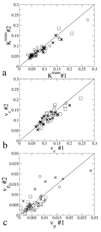
K^trans, v_e and v_p from scan #1 and scan #2 plotted against each other. Parameters estimated by the MRTM individual AIF, the MRTM population AIF and the Parker population AIF were respectively plotted with circle, cross and square. Solid lines show the line of equality.

Table 2.

Reproducibility assessment of parameters for the N=16 patients.

	Parameter	MRTM individualAIF	MRTM populationAIF	Parker populationAIF
Ktrans	global mean μ(min−1)	0.088	0.080	0.087
	Kendall’s τ	0.17, p=0.40	0.37, p=0.052	0.62,p=0.0005
	Mean difference (±SD)	0.002(±0.018)	−0.006(±0.013)	−0.006(±0.019)
	Repeatability(95%CI)a (min−1)	0.035	0.028	0.037
	wCV a (%)	14.4%	12.5%	15.5%
	wCV b (%)	15.1%	10.5%	11.7%
	Repeatability(95% CI) b (%)	41.8%	29.0%	32.4%
ve	global mean μ	0.114	0.110	0.133
	Kendall’s τ	0.15, p=0.45	0.32, p=0.096	0.30,p=0.12
	mean difference (±SD)	−0.003(±0.015)	−0.005(±0.016)	−0.005(±0.023)
	Repeatability(95%CI) a	0.029	0.033	0.046
	wCV a (%)	9.3%	10.8%	12.4%
	wCV b (%)	9.9%	11.0%	12.7%
	Repeatability(95% CI) b (%)	27.3%	30.4%	35.1%
vp	global mean μ	0.0068	0.0088	0.0043
	Kendall’s τ	0.12,p=0.56	0.37,p=0.052	0.32,p=0.096
	mean difference (±SD)	−0.0002(± 0.0033)	0.0003(±0.0037)	−0.0001(±0.0021)
	Repeatability(95%CI)a	0.0062	0.0071	0.0040
	wCV a (%)	33.0%	29.1%	33.7%
	wCV b (%)	26.1%	34.6%	37.6%
	Repeatability(95% CI) b (%)	72.2%	95.8%	104.1%

^aUnder absolute repeatability model, preferred when p<0.05 under Kendall’s τ test.

^bUnder relative repeatability model, preferred when p ≥ 0.05 under Kendall’s τ test. The results based on the preferred repeatability model were highlighted by bolding.

The fact that different repeatability models are most applicable for K^trans determined with different AIF estimation methods complicates the comparison of the wCV. Nevertheless, for K^trans, MRTM population AIF gave the smallest wCV under both repeatability models. For v_e, the MRTM individual AIF gave the smallest wCV. For v_p, the wCV were very close between the three AIFs. The MRTM population AIF always gave a smaller wCV than the Parker population AIF; and it either gave very close or smaller wCV compared to the MRTM individual AIF. Overall the MRTM population AIF provided most reproducible results even though the difference in wCV between the three different AIFs was fairly small. The parameter v_p was considerably less reproducible than K^trans, and v_e.

According to Table 2, on average the Parker population AIF gave a considerably larger estimate of v_e, and a smaller estimate of v_p compared to the other two AIFs. However, there was excellent correlation between the parameters estimated by the three AIFs, with all correlation coefficients > 0.73 (Table 3).

Table 3.

Correlation coefficient between parameters estimated by the MRTM individual AIF (AIF_MI), the MRTM population AIF (AIF_MP) and the Parker population AIF (AIF_PP) in the 32 experiments.

	AIFMI vs AIFMP	AIFMI vs AIFPP	AIFMP vs AIFPP
Ktrans	0.93	0.85	0.99
ve	0.77	0.78	0.99
vp	0.78	0.73	0.83

DISCUSSION AND CONCLUSIONS

With a multiple reference tissue method (MRTM) under the extended Tofts model, we estimated the local tissue AIF in 32 DCE-MRI experiments from 16 patients using the contrast agent enhancement data from tumor sub-regions and muscle. Similar to the finding in many other studies (11,12), considerable intra-patient variability and large inter-patient variability were observed in the 32 individual AIFs. From the 32 MRTM individual AIFs, we also calculated the average AIF across this population. The MRTM individual AIFs all showed a first pass and a washout phase, similar to directly measured AIFs in the literature (31,32). The MRTM population AIF clearly showed the recirculation second pass.

In this study, the MRTM used the estimated C_t(t) from tumor sub-regions and muscle to estimate the AIF under the extended Tofts model. Several possible sources of variability in the estimated AIF include biologic variability, the limitation of the DCE-MRI models used, errors in the estimation of C_t(t), and errors in the scaling of the AIF. The most important source of biologic variability under the short interval between scans here is likely day to day variability in the CO. The coefficient of variation of CO was reported to be about 10% in Table 2 in (33). In regards to DCE-MRI models, Eq. [2] and the extended Tofts model used in this study assume a fast exchange limit (FXL), which is not always valid. As the contrast agent concentration in the tissue increases, the water exchange system between the tissue compartments will deviate from the FXL, and this can lead to some errors in the estimated AIF when a DCE-MRI model which assumes the FXL is applied to the MRTM instead. Recently, “shutter-speed models,”(34,35) have been proposed to address the nonlinear effect caused by deviation from the FXL, those models can potentially be applied to the MRTM. Errors in the estimation of C_t(t) can also be introduced by measurement white noise, RF inhomogeneity and non-uniform flip angle profile (36) in the slice direction for 2D-excitation, and the approximation used in Eq. [3]. In addition, the lack of a pre-contract T₁ measurement is a limitation of this study, if the native T₁ value of muscle was not equal to the literature value in a particular experiment, all the C_t(t) as well as the AIF estimated would be off by a common factor. Finally, we obtained the scale of the MRTM AIF by using the C_t(t) from muscle ROI and assuming its v_e to be 0.08 as has been observed in rodent experimental studies utilizing directly measured AIFs and the Tofts model (27). The fact that our MRTM population AIF had a very similar magnitude to the Parker population AIF, which is derived from human arterial measured AIFs, at the initial washout provides support for the assumed v_e. However, in a particular experiment deviation of muscle v_e from 0.08 will introduce errors in the scaling of the MRTM individual AIF. Nevertheless, the large within patient variability observed in the AIF from some patients, such as patient #2 would infer such large differences in CO (8.42 l/min versus 11.11 l/min) that technical and not just biologic factors likely played a role and further studies will have to clarify which of the above noted factors is most critical.

Compared to the population AIF reported by Parker et al from 67 AIFs directly measured by imaging the arteries with DCE-MRI, our MRTM population AIF had a lower and more dispersed first pass peak. The larger dispersion might be partly caused by the slower contrast agent injection rate used in our experiments (2 ml/sec versus 3 ml/sec). More likely it is due to the unique population studied here; namely prostate cancer bone metastases. Most important, however, the MRTM AIF is a local tissue AIF, and larger dispersion is expected as the contrast agent travels from remote major arteries to the capillary (37). In the MRTM population AIF, the area under the first pass was nearly 50% larger than the Parker population AIF. For the Parker population AIF, the inferred CO of 10.5 l/min is much larger than the average CO for adults at rest reported in the literature as 6.5 l/min (38). This suggests that its first pass might be slightly under-estimated, possibly due to inadequate temporal resolution as pointed out by the authors (11) or other artifacts such as T₂* effects. The inferred CO of the MRTM population AIF (6.1 l/min) as well as the individual CO is consistent with the range of CO expected for human adults at rest, which provides indirect support for the AIF estimated by the MRTM.

The MRTM population AIF had slower washout rate in the later portion of the washout phase than the Parker population AIF. Physical states such as the cardiac output, blood flow distribution in organs, and kidney function will all affect the washout rate (39). The difference in the washout rate might thus be partly caused by biologic and medical differences between the two populations. In addition, Parker et al used an exponential function to fit the washout phase, and close inspection of Fig. 3 in (11) showed that it underestimated the original data in the later part of the washout phase. In previous pharmacokinetic experiments, a bi-exponential function (9) was more commonly used to fit the washout phase. Nevertheless, the shape of the washout phase of the Parker as well as the MRTM population AIF are very close to directly measured AIFs in the literature. Furthermore, in a previous experimental study of the MRTM using 3D pulse sequence (40), it has been shown that the AIF estimated by the MRTM matched well with the AIF directly measured from arteries in the washout phase. This could not be replicated in this study, because a 2D pulse sequence was used, which introduced significant pulsatile artifacts due to inflow effect making direct AIF measurement impossible.

The MRTM AIFs gave a better fit to the observed contrast agent concentration data than the Parker population AIF. It is likely that this is due to the fact that it reflects a local tissue AIF in the specific population studied rather than an AIF from a different population derived from remote arteries. Other explanations include differences in the experimental setup such as the contrast agent injection profile and the use of a single exponential function to fit the washout phase in the Parker population AIF.

In this study, the MRTM individual AIFs gave estimates of K^trans with reproducibility similar to that of the Parker population AIF, and a more reproducible estimate of v_e. Those features of reproducibility may be related to the methodology used in this study. For example, as discussed above some source of errors will cause the C_t(t) and the estimated MRTM individual AIF to be off by a common factor. When individual AIFs are used, such measurement errors would get cancelled out in the derived estimated parameters; however, when fixed population AIFs are used, the resultant measurement errors are proportional to the parameter magnitude. There is some evidence for this in Table 2. When the population AIFs were used the p-value for Kendall’s τ tests, were all less than or equal to 0.12, which suggests that measurement errors in the estimated parameters were weakly proportional to the parameter magnitude. These features, along with the aforementioned better fit of the observed concentration versus time curves, suggest that individual MRTM AIFs have a distinct advantage and may provide more accurate kinetic parameter estimates in DCE-MRI studies.

Nevertheless, a population AIF is easier to apply, has higher SNR than individual AIFs, and does not have the random errors present in the MRTM individual AIFs (19), all of which should boost the reproducibility of the estimated kinetic parameters (11). In fact, in this study, overall the MRTM population AIF gave the most reproducible parameter estimates. Simulation studies have also suggested that the random error in the estimated MRTM AIF increases with the measurement errors of the dynamic data (19), such as might be expected with motion artifact. One additional unique advantage of a population AIF derived from the imaged cohort is that it is likely to better reflect the unique characteristics of that cohort, such as prostate cancer bone metastases studied here. These considerations, the observed good reproducibility obtained with the population AIFs, and the strong correlation between the parameters estimated by the population AIFs with the MRTM individual AIFs (Table 3) suggest that study specific population AIFs might be especially useful when relative changes in the parameters are more important than absolute values (2).

Finally, it is notable that the wCV of v_p in this study was much larger than in a previous study despite the fact that the repeatability of K^trans and v_e was similar (11). This is likely due to the fact that the average v_p of tumors prostate bone metastases studied here was close to zero and the previous study included a variety of different tumors. It is well known that some tumors such as renal cell carcinoma have much larger v_p value than other tumors.

In conclusion, the MRTM is a practical method for obtaining reproducible kinetic parameters from DCE-MRI clinical studies. Major advantages of the MRTM are that it does not require a major artery in the FOV and is dependent on fewer assumptions. It additionally estimates the individual local tissue AIF. For DCE-MRI data with good SNR and relatively high temporal resolution, the MRTM AIF gives better fits and equally reproducible estimate of kinetic parameters compared to a previous reported population AIF. The individual MRTM AIFs can also be used to obtain a mean local tissue AIF for a unique population, such as prostate cancer metastatic to bone, which can provide a more reproducible estimate of DCE-MRI parameters than the population AIF measured from major arteries in another population. In sum, this study suggests that the MRTM can be applied to DCE-MRI studies of bone metastases from prostate cancers to provide an AIF from which reproducible quantitative DCE-MRI parameters can be derived. The MRTM might be applied to other DCE-MRI studies of cancers thus helping standardize DCE-MRI studies in cancer patients.

References

- 1.Padhani AR. Dynamic contrast-enhanced MRI in clinical oncology: current status and future directions. J Magn Reson Imaging. 2002;16(4):407–422. doi: 10.1002/jmri.10176. [DOI] [PubMed] [Google Scholar]
- 2.Morgan B, Thomas AL, Drevs J, Hennig J, Buchert M, Jivan A, Horsfield MA, Mross K, Ball HA, Lee L, Mietlowski W, Fuxuis S, Unger C, O'Byrne K, Henry A, Cherryman GR, Laurent D, Dugan M, Marme D, Steward WP. Dynamic contrast-enhanced magnetic resonance imaging as a biomarker for the pharmacological response of PTK787/ZK 222584, an inhibitor of the vascular endothelial growth factor receptor tyrosine kinases, in patients with advanced colorectal cancer and liver metastases: results from two phase I studies. J Clin Oncol. 2003;21(21):3955–3964. doi: 10.1200/JCO.2003.08.092. [DOI] [PubMed] [Google Scholar]
- 3.Liu G, Rugo HS, Wilding G, McShane TM, Evelhoch JL, Ng C, Jackson E, Kelcz F, Yeh BM, Lee FT, Jr, Charnsangavej C, Park JW, Ashton EA, Steinfeldt HM, Pithavala YK, Reich SD, Herbst RS. Dynamic contrast-enhanced magnetic resonance imaging as a pharmacodynamic measure of response after acute dosing of AG-013736, an oral angiogenesis inhibitor, in patients with advanced solid tumors: results from a phase I study. J Clin Oncol. 2005;23(24):5464–5473. doi: 10.1200/JCO.2005.04.143. [DOI] [PubMed] [Google Scholar]
- 4.Tofts PS, Brix G, Buckley DL, Evelhoch JL, Henderson E, Knopp MV, Larsson HB, Lee TY, Mayr NA, Parker GJ, Port RE, Taylor J, Weisskoff RM. Estimating kinetic parameters from dynamic contrast-enhanced T(1)-weighted MRI of a diffusable tracer: standardized quantities and symbols. J Magn Reson Imaging. 1999;10(3):223–232. doi: 10.1002/(sici)1522-2586(199909)10:3<223::aid-jmri2>3.0.co;2-s. [DOI] [PubMed] [Google Scholar]
- 5.Leach MO, Brindle KM, Evelhoch JL, Griffiths JR, Horsman MR, Jackson A, Jayson GC, Judson IR, Knopp MV, Maxwell RJ, McIntyre D, Padhani AR, Price P, Rathbone R, Rustin GJ, Tofts PS, Tozer GM, Vennart W, Waterton JC, Williams SR, Workman P. The assessment of antiangiogenic and antivascular therapies in early-stage clinical trials using magnetic resonance imaging: issues and recommendations. Br J Cancer. 2005;92(9):1599–1610. doi: 10.1038/sj.bjc.6602550. [DOI] [PMC free article] [PubMed] [Google Scholar]
- 6.Wendland MF, Saeed M, Yu KK, Roberts TP, Lauerma K, Derugin N, Varadarajan J, Watson AD, Higgins CB. Inversion recovery EPI of bolus transit in rat myocardium using intravascular and extravascular gadolinium-based MR contrast media: dose effects on peak signal enhancement. Magn Reson Med. 1994;32(3):319–329. doi: 10.1002/mrm.1910320307. [DOI] [PubMed] [Google Scholar]
- 7.Chen JJ, Smith MR, Frayne R. The impact of partial-volume effects in dynamic susceptibility contrast magnetic resonance perfusion imaging. J Magn Reson Imaging. 2005;22(3):390–399. doi: 10.1002/jmri.20393. [DOI] [PubMed] [Google Scholar]
- 8.Ivancevic MK, Zimine I, Foxall D, Lecoq G, Righetti A, Didier D, Vallee JP. Inflow effect in first-pass cardiac and renal MRI. J Magn Reson Imaging. 2003;18(3):372–376. doi: 10.1002/jmri.10363. [DOI] [PubMed] [Google Scholar]
- 9.Weinmann HJ, Laniado M, Mutzel W. Pharmacokinetics of GdDTPA/dimeglumine after intravenous injection into healthy volunteers. Physiol Chem Phys Med NMR. 1984;16(2):167–172. [PubMed] [Google Scholar]
- 10.Tofts PS, Kermode AG. Measurement of the blood-brain barrier permeability and leakage space using dynamic MR imaging. 1. Fundamental concepts. Magn Reson Med. 1991;17(2):357–367. doi: 10.1002/mrm.1910170208. [DOI] [PubMed] [Google Scholar]
- 11.Parker GJ, Roberts C, Macdonald A, Buonaccorsi GA, Cheung S, Buckley DL, Jackson A, Watson Y, Davies K, Jayson GC. Experimentally-derived functional form for a population-averaged high-temporal-resolution arterial input function for dynamic contrast-enhanced MRI. Magn Reson Med. 2006;56(5):993–1000. doi: 10.1002/mrm.21066. [DOI] [PubMed] [Google Scholar]
- 12.Port RE, Knopp MV, Brix G. Dynamic contrast-enhanced MRI using Gd-DTPA: interindividual variability of the arterial input function and consequences for the assessment of kinetics in tumors. Magn Reson Med. 2001;45(6):1030–1038. doi: 10.1002/mrm.1137. [DOI] [PubMed] [Google Scholar]
- 13.Kovar DA, Lewis M, Karczmar GS. A new method for imaging perfusion and contrast extraction fraction: input functions derived from reference tissues. J Magn Reson Imaging. 1998;8(5):1126–1134. doi: 10.1002/jmri.1880080519. [DOI] [PubMed] [Google Scholar]
- 14.Padhani AR, Hayes C, Landau S, Leach MO. Reproducibility of quantitative dynamic MRI of normal human tissues. NMR Biomed. 2002;15(2):143–153. doi: 10.1002/nbm.732. [DOI] [PubMed] [Google Scholar]
- 15.Walker-Samuel S, Parker CC, Leach MO, Collins DJ. Reproducibility of reference tissue quantification of dynamic contrast-enhanced data: comparison with a fixed vascular input function. Phys Med Biol. 2007;52(1):75–89. doi: 10.1088/0031-9155/52/1/006. [DOI] [PubMed] [Google Scholar]
- 16.Yang C, Karczmar GS, Medved M, Stadler WM. Estimating the arterial input function using two reference tissues in dynamic contrast-enhanced MRI studies: fundamental concepts and simulations. Magn Reson Med. 2004;52(5):1110–1117. doi: 10.1002/mrm.20243. [DOI] [PubMed] [Google Scholar]
- 17.Yankeelov TE, Luci JJ, Lepage M, Li R, Debusk L, Lin PC, Price RR, Gore JC. Quantitative pharmacokinetic analysis of DCE-MRI data without an arterial input function: a reference region model. Magn Reson Imaging. 2005;23(4):519–529. doi: 10.1016/j.mri.2005.02.013. [DOI] [PubMed] [Google Scholar]
- 18.Yankeelov TE, Luci JJ, DeBusk LM, Lin PC, Gore JC. Incorporating the effects of transcytolemmal water exchange in a reference region model for DCE-MRI analysis: theory, simulations, and experimental results. Magn Reson Med. 2008;59(2):326–335. doi: 10.1002/mrm.21449. [DOI] [PMC free article] [PubMed] [Google Scholar]
- 19.Yang C, Karczmar GS, Medved M, Stadler WM. Multiple reference tissue method for contrast agent arterial input function estimation. Magn Reson Med. 2007;58(6):1266–1275. doi: 10.1002/mrm.21311. [DOI] [PubMed] [Google Scholar]
- 20.Riabkov DY, Di Bella EV. Estimation of kinetic parameters without input functions: analysis of three methods for multichannel blind identification. IEEE Trans Biomed Eng. 2002;49(11):1318–1327. doi: 10.1109/TBME.2002.804588. [DOI] [PubMed] [Google Scholar]
- 21.Riabkov DY, Di Bella EV. Blind identification of the kinetic parameters in three-compartment models. Phys Med Biol. 2004;49(5):639–664. doi: 10.1088/0031-9155/49/5/001. [DOI] [PubMed] [Google Scholar]
- 22.Port RE, Knopp MV, Hoffmann U, Milker-Zabel S, Brix G. Multicompartment analysis of gadolinium chelate kinetics: blood-tissue exchange in mammary tumors as monitored by dynamic MR imaging. J Magn Reson Imaging. 1999;10(3):233–241. doi: 10.1002/(sici)1522-2586(199909)10:3<233::aid-jmri3>3.0.co;2-m. [DOI] [PubMed] [Google Scholar]
- 23.Medved M, Karczmar G, Yang C, Dignam J, Gajewski TF, Kindler H, Vokes E, MacEneany P, Mitchell MT, Stadler WM. Semiquantitative analysis of dynamic contrast enhanced MRI in cancer patients: Variability and changes in tumor tissue over time. J Magn Reson Imaging. 2004;20(1):122–128. doi: 10.1002/jmri.20061. [DOI] [PubMed] [Google Scholar]
- 24.Bydder GM, Hajnal JV, Young IR. Use of the inversion recovery pulse sequence. In: Stark DD, Bradley WG, editors. Magnetic Resonance Imaging. St. Louis: William G. Mosby; 1999. pp. 69–86. [Google Scholar]
- 25.Wong KP, Feng DG, Meikle SR, Fulham MJ. Segmentation of dynamic PET images using cluster analysis. IEEE T Nucl Sci. 2002;49(1):200–207. [Google Scholar]
- 26.Donahue KM, Weisskoff RM, Parmelee DJ, Callahan RJ, Wilkinson RA, Mandeville JB, Rosen BR. Dynamic Gd-DTPA enhanced MRI measurement of tissue cell volume fraction. Magn Reson Med. 1995;34(3):423–432. doi: 10.1002/mrm.1910340320. [DOI] [PubMed] [Google Scholar]
- 27.Yankeelov TE, Cron GO, Addison CL, Wallace JC, Wilkins RC, Pappas BA, Santyr GE, Gore JC. Comparison of a reference region model with direct measurement of an AIF in the analysis of DCE-MRI data. Magn Reson Med. 2007;57(2):353–361. doi: 10.1002/mrm.21131. [DOI] [PubMed] [Google Scholar]
- 28.Thompson HK, Jr, Starmer CF, Whalen RE, McIntosh HD. Indicator Transit Time Considered as a Gamma Variate. Circ Res. 1964;14:502–515. doi: 10.1161/01.res.14.6.502. [DOI] [PubMed] [Google Scholar]
- 29.Hamilton WF, Riley KL, Attyah AM, Cournand A, Fowell DM, Himmelstein A, Noble RP, Remington JW, Richards DW, Wheeler NC, Whitham AC. Comparison of the Fick and Dye indicator methods of measuring cardiac output in man. Am J Physiol. 1948;153:309. doi: 10.1152/ajplegacy.1948.153.2.309. [DOI] [PubMed] [Google Scholar]
- 30.Garrett JS, Lanzer P, Jaschke W, Botvinick E, Sievers R, Higgins CB, Lipton MJ. Measurement of cardiac output by cine computed tomography. Am J Cardiol. 1985;56(10):657–661. doi: 10.1016/0002-9149(85)91030-6. [DOI] [PubMed] [Google Scholar]
- 31.Li KL, Zhu XP, Waterton J, Jackson A. Improved 3D quantitative mapping of blood volume and endothelial permeability in brain tumors. J Magn Reson Imaging. 2000;12(2):347–357. doi: 10.1002/1522-2586(200008)12:2<347::aid-jmri19>3.0.co;2-7. [DOI] [PubMed] [Google Scholar]
- 32.Fritz-Hansen T, Rostrup E, Larsson HB, Sondergaard L, Ring P, Henriksen O. Measurement of the arterial concentration of Gd-DTPA using MRI: a step toward quantitative perfusion imaging. Magn Reson Med. 1996;36(2):225–223. doi: 10.1002/mrm.1910360209. [DOI] [PubMed] [Google Scholar]
- 33.Montani JP, Mizelle HL, Van Vliet BN, Adair TH. Advantages of continuous measurement of cardiac output 24 h a day. Am J Physiol. 1995;269(2 Pt 2):H696–703. doi: 10.1152/ajpheart.1995.269.2.H696. [DOI] [PubMed] [Google Scholar]
- 34.Yankeelov TE, Rooney WD, Li X, Springer CS., Jr Variation of the relaxographic "shutter-speed" for transcytolemmal water exchange affects the CR bolus-tracking curve shape. Magn Reson Med. 2003;50(6):1151–1169. doi: 10.1002/mrm.10624. [DOI] [PubMed] [Google Scholar]
- 35.Li X, Rooney WD, Springer CS., Jr A unified magnetic resonance imaging pharmacokinetic theory: intravascular and extracellular contrast reagents. Magn Reson Med. 2005;54(6):1351–1359. doi: 10.1002/mrm.20684. [DOI] [PubMed] [Google Scholar]
- 36.Parker GJ, Barker GJ, Tofts PS. Accurate multislice gradient echo T(1) measurement in the presence of non-ideal RF pulse shape and RF field nonuniformity. Magn Reson Med. 2001;45(5):838–845. doi: 10.1002/mrm.1112. [DOI] [PubMed] [Google Scholar]
- 37.Calamante F, Gadian DG, Connelly A. Delay and dispersion effects in dynamic susceptibility contrast MRI: simulations using singular value decomposition. Magn Reson Med. 2000;44(3):466–473. doi: 10.1002/1522-2594(200009)44:3<466::aid-mrm18>3.0.co;2-m. [DOI] [PubMed] [Google Scholar]
- 38.Wade OL, Bishop JM. Cardiac output and regional blood flow. Philadelphia, PA: F.A. Davis Co; 1962. pp. 86–95. [Google Scholar]
- 39.Krejcie TC, Henthorn TK, Niemann CU, Klein C, Gupta DK, Gentry WB, Shanks CA, Avram MJ. Recirculatory pharmacokinetic models of markers of blood, extracellular fluid and total body water administered concomitantly. J Pharmacol Exp Ther. 1996;278(3):1050–1057. [PubMed] [Google Scholar]
- 40.Yang C, Stadler WM, Medved M, Karczmar GS. Tumor Arterial Input Function (AIF) estimation in DCE-MRI studies using a multiple reference tissue method; Proceedings of the 14th Annual Meeting of ISMRM; Seattle, USA. 2006. p. 384. [Google Scholar]