Abstract
Empirical Bayes (“post hoc”) estimates (EBEs) of ηs provide modelers with diagnostics: the EBEs themselves, individual prediction (IPRED), and residual errors (individual weighted residual (IWRES)). When data are uninformative at the individual level, the EBE distribution will shrink towards zero (η-shrinkage, quantified as 1-SD(ηEBE)/ω), IPREDs towards the corresponding observations, and IWRES towards zero (ε-shrinkage, quantified as 1-SD(IWRES)). These diagnostics are widely used in pharmacokinetic (PK) pharmacodynamic (PD) modeling; we investigate here their usefulness in the presence of shrinkage. Datasets were simulated from a range of PK PD models, EBEs estimated in non-linear mixed effects modeling based on the true or a misspecified model, and desired diagnostics evaluated both qualitatively and quantitatively. Identified consequences of η-shrinkage on EBE-based model diagnostics include non-normal and/or asymmetric distribution of EBEs with their mean values (“ETABAR”) significantly different from zero, even for a correctly specified model; EBE–EBE correlations and covariate relationships may be masked, falsely induced, or the shape of the true relationship distorted. Consequences of ε-shrinkage included low power of IPRED and IWRES to diagnose structural and residual error model misspecification, respectively. EBE-based diagnostics should be interpreted with caution whenever substantial η- or ε-shrinkage exists (usually greater than 20% to 30%). Reporting the magnitude of η- and ε-shrinkage will facilitate the informed use and interpretation of EBE-based diagnostics.
Key words: empirical Bayes estimate, model building, model evaluation, NONMEM, shrinkage
INTRODUCTION
Model-based analysis has lately become a method of choice for analyzing the outcome from clinical trials in drug development. The model(s) explaining underlying pharmacokinetics (PK) and pharmacodynamics (PD) of a therapeutic agent as well as disease progression is used for data description, interpretation, and simulation of future scenarios, as well as decision-making. Thus, the choice of an adequate model is a crucial but often not straightforward procedure. The model building process is difficult and involves testing, evaluating, and diagnosing a range of plausible models with a major aim to make an adequate inference from the observed data, summarized as parameter estimates, variability estimates, and significant covariates (1).There are several tools assisting modelers in a model building process, including graphical diagnostics (1–3).
Graphical displays are extensively used during the model building process and are considered an essential tool for data visualization, inspection of model adequacy, and assumption testing. Graphical diagnostics are considered a powerful and intuitive visual method to be used not only by modelers but also as a communicating tool. The US Food and Drug Administration and the European Committee for Medicinal Products for Human use guidances explicitly mention the utility of graphical diagnostics. Specifically mentioned in both guidances are graphical diagnostics based on individual parameter estimates (4–6). The individual parameter estimates in non-linear mixed effects are estimated using the Bayesian methodology, and they are generally referred to as an empirical Bayes estimates (EBEs). The use of the phrase ‘empirical Bayes’ emphasizes that the parameters for the prior distribution are estimated from the data and are used as if they were known to obtain the posterior distribution. At one extreme, with no observations available, the patient will be regarded as a typical patient. At the other extreme, when data for an individual goes towards infinity, the prior will have marginal impact; in between these extremes, both factors will contribute, and depending on the relative variability (including both, between, and within subject variability), individual estimates could be closer either to the population mean or to the true individual parameter value (7–9).
Although the advantages and strengths of graphical diagnostics have been justified and stressed on several occasions, shortcomings have not been systematically explored (10). In this work, we investigate the informative value of the EBE-based diagnostics and how their usefulness depends on the individual data richness. Additionally, circumstances which are likely to misguide modelers towards making erroneous decisions in model development, relating to choice of structural, covariate, and stochastic model components, are underlined.
METHODS
Empirical Bayes Estimation and Notation
Derivation of individual parameter estimates (EBEs), denoted for an individual j as a vector of s model parameters Pj = (pj1,pj2…pjs), requires quantities such as (1) typical individual estimates denoted as a vector of θ = (θ1,…θs); (2) the magnitude of inter-individual variability of parameters in question, variances (ω21,…,ωs2), and covariances of the Ω-matrix; as well as (3) the magnitude (variance) of residual variability (σ2) to be known. The number of variance parameters (ω2) does not necessarily need to be the same as the number of typical parameter estimates (θ). Then, in individual j, the kth parameter’s deviation from the typical parameter value in the population can be denoted ηjk. In parametric non-linear mixed effect modeling, the shape of the distribution of the ηs is assumed to be normal. Commonly, to avoid negative parameter values, the parameter distribution is log-normally transformed using the relationship described in Eq. 1 where ηjk enters nonlinearly into the expression for the parameter in order to appropriately mimic the parameter distribution shape in the population. Also, as Eq. 1 is straightforward, the ηjk value is often referred to as an individual parameter. Thus, considering Eq. 1, the vector ηk will be used as an indicator for the individual parameter throughout the remainder of this communication.
 |
1 |
For individual j, individual parameter  can be estimated from the observed data vector yji = (yj1, yj2,…,yjn), n being the number of observations within an individual and known prior parameter distribution. Detailed derivation of this estimation procedure is available elsewhere (7,11).
With ŷji, we denote a model prediction of yji, defined as a function of parameter vector Pj and Xji, Xji being the vector of independent variables (such as time and dose covariates) related to yji (Eq. 2).
 |
2 |
Definition of Diagnostic Variables
In this communication, ŷji is referred to as an individual prediction (IPRED) and to ηEBE,jk as the EBE. Another useful term, the individual weighted residual (IWRES), is calculated following Eq. 3. By using the standard deviation of the residual variability as a weighting factor, the IWRES distribution is standardized to have a zero mean and unit variance expectation when the model and parameters are correct at the individual level.
 |
3 |
Definition of η- and ε-Shrinkage
If the population model is adequate, the quality of the individual parameter estimate will depend heavily on the observed data available. When data are sparse and less informative on individual parameters, it is expected that the EBEs will deviate less from the population mean, which will result in a difference in the EBE and priors distribution, mainly in terms of decreased variance of EBEs but also with possible distortions of the distribution shape. In an extreme case of no data available on a particular individual, the individual’s EBE will be equal to the population value. So, the variance of EBE distribution is shrinking towards zero as the quantity of information at the individual level diminishes, a phenomenon defined as η-shrinkage (shη). Similarly, as individual parameter estimate tend towards the true individual parameter in case of informative data, IWRES distribution approaches a normal distribution with zero mean and unit variance. Conversely, as data diminishes, the IWRES distribution shrinks towards zero. We define this phenomenon as ε-shrinkage (shε) and is sometimes also called “overfitting”.
η- and ε-shrinkage are calculated using Eqs. 4 and 5. A shrinkage magnitude of zero, i.e., no shrinkage, corresponds to the situation when the model is correct and individual data is sufficiently abundant so that individual parameter estimates mimic the true individual parameter estimates, and a magnitude of one is the opposite case when data contain virtually no information about the parameters in question and the individual parameter values approach the typical parameter value.
 |
4 |
 |
5 |
Simulations
General Description
The influence of shrinkage on EBE-based diagnostics was assessed via ordinary (n ≤ 10) or Monte Carlo (MC; n = 100) PK or PD model simulation–estimation procedures using non-linear mixed effects modeling (NONMEM; 12). The model summary is given in Table I. Data sets with different information content were created by altering the number (sample frequency) and location (sampling time) of samples. Each scenario defined with a certain model, and study design underwent multiple simulations. If not specified otherwise below, each simulated dataset contained 1,000 subjects. Thereafter, the EBEs were estimated using either the true and/or an intentionally misspecified model for each dataset using Bayesian estimation (i.e., MAXEVAL = 0 option) in NONMEM. In this estimation, the prior information, i.e., population parameter estimates, variances, covariances, and residual variability were fixed to the same values used for simulations of the data sets, whenever misspecification was not introduced.
Table I.
Summary of Models used for Simulations
| Model indexing | Model description |
|---|---|
| Model 1 | One compartment i.v. bolus model |
| Model 2 | One compartment i.v. bolus model with Michaelis–Menten elimination |
| Model 3 | Two compartment i.v. bolus model |
| Model 4 | One compartment model with first order absorption |
| Model 5 | One compartment model with zero order absorption |
| Model 6 | One compartment model with transit compartment absorption |
| Model 7 | Two compartment model with first order absorption |
| Model 8 | Emax model |
| Model 9 | Sigmoidal Emax model |
| Model 10 | Indirect response model |
i.v. intravenous
Based on estimated EBEs, IPREDs, and IWRES, graphical diagnostics were created and subsequently inspected for trends or indications of model misspecification. Also, the extent of η- and ε-shrinkage was calculated for these estimated EBE or IWRES distributions. Overall, the relationship between the extent of shrinkage and informativeness of diagnostics was assessed both qualitatively, i.e., by visual inspection of whether or not the resulting plot indicated the expected pattern, and quantitatively, i.e., to determine at what shrinkage magnitude a particular diagnostics lose its utility.
Commonly used EBE diagnostics were explored. A brief description of these diagnostics as well as the methodology used to study their informativeness for each case is given below.
Specific Description
Shape of EBE distribution
Description
A visual diagnostic often used to inspect the EBE distribution and to confirm the normality assumption is either a histogram or, preferably, a quantile–quantile-plot (qq-plot), where deviations from normality can be detected.
Methodology
Multiple datasets (n = 10 for each unique design) were simulated from a PK model (one compartment model with first order absorption, model 4) using different study designs with respect to sampling frequency (2–10) and sampling times. The EBEs were estimated using the true model for each dataset. EBE and IWRES distributions were visualized and compared to the true normal distribution using qq-plots.
-
2.
ETABAR outcome
Description
A hypothesis test if the mean value of EBEs is significantly different from zero is performed at each run, and the p value of this test is reported in the so-called “ETABAR outcome” from NONMEM. A significant ETABAR is considered as an indication for a potential model misspecification.
Methodology
Data sets were simulated from one compartment intravenous bolus model (model 1) and one compartment model with first order absorption (model 4) to study this diagnostic. The simulated datasets comprised two and three samples each for models 1 and 2, respectively. Two conditions were studied: (1) dependence of ηCL ETABAR on the time of the last sample in model 1 and (2) dependence of the ηka ETABAR on the time of the first sample in model 2. For condition 1, seven (7) MC simulation–estimation studies were performed using different study designs in which the last sample was positioned at the time equal to the 0.67, 1, 2, 3, 4, 6, and 8 of the disposition half-life (t1/2 = 3 h) for seven MC studies. Similarly, for condition 2, eight MC simulation–estimation studies was performed in which the first samples was positioned to be equal to the 0.25, 0.5, 0.75, 1, 1.5, 2, 2.5, and 4 absorption half-lives (t1/2abs = 1 h). Each MC involved 100 replicates of simulated datasets. The true model was fitted to the simulated data using First Order Conditional Estimation method (FOCE) in NONMEM VI.
-
3.
EBE versus EBE plots
Description
This diagnostic is often used for inspection of the correlation between individual parameter estimates. If the plot indicates a markedly non-zero correlation for a model where the population correlation value was fixed to zero, the correlation is generally tested in the model for its significance. If the plot indicates zero correlation for a model where the population correlation value was also zero, the correlation is often not tested for its significance.
Methodology
Two conditions were studied: the value of EBEs to (1) indicate correlation if it is truly present and/or (2) correctly determining when the correlation is not present. Condition 1 was studied using model 1, in which the true correlation between individual parameters of ηCL and ηV was 0.75. Datasets were simulated using this model and different study designs. For each design, ten replicates were simulated. The model with true parameter estimates but no correlation was used to estimate EBEs. The expectation is that EBE versus EBE plot will indicate parameter correlation. Correlation between EBEs values for ηCL and ηV was computed for each EBE versus EBE plot. Condition 2 was studied using model 4 and model 9 (an Emax model). In these models, the true correlation between all individual parameters was zero. All study conditions were equivalent to the study described above; however, the true model with no correlation was used to estimate EBEs.
-
4.
EBE versus covariate plots
Description
This diagnostic is used for inspection of relationships between parameters and covariates. When a large number of covariates are available, this diagnostic enables a quick screening of relationships. Only indicated relationships are often subsequently estimated directly in the population model. EBEs are also used in automated procedures such as the generalized additive modeling (13) and to investigate the shape of the covariate-parameter relationship.
Methodology
The utility of EBEs to correctly indicate the EBE-covariate relationship when (1) it is truly present and (2) when the covariate relationship is not present were studied using model 4. A direct relationship between typical value of volume of distribution and weight was used for simulations. Multiple datasets were simulated under different study designs, where early observations were censored sequentially. A model with no covariate relationship was fitted to the data and used to estimate EBEs which were subsequently plotted versus the covariate (weight). Correlation between EBEs and weight as well as the slope of EBE versus weight relationships were calculated for each data set.
-
5.
Dependent variable (DV) versus IPRED plot
Description
This is a commonly used diagnostic for detection of (structural) model misspecification. Its usefulness, compared to the DV versus population prediction (PRED) plot, comes from separating different sources of variability.
Methodology
A range of models was used to simulate multiple datasets, which were subsequently analyzed with structurally misspecified models. The examples involve the following pairs of models (first model in a pair is used for simulation, second for estimation): (1) sigmoidal Emax model–Emax model (models 9 and 8), (2) transit compartment absorption model–first order absorption model (model 6 and 4), (3) two compartment model–one compartment model (models 3 and 1), (4) one compartment model with first order absorption–one compartment model with zero order absorption (models 4 and 5), and (5) one compartment model with Michaelis–Menten elimination–one compartment model with linear elimination (models 2 and 1). For each condition, multiple datasets with different number of observations were simulated. IPREDs were derived from the misspecified model.
-
6.
|IWRES| versus IPRED plot
Description
This is a commonly used diagnostic for assessing the residual error model. An appropriate residual error model should be associated with a horizontal regression line with no slope.
Methodology
Multiple datasets based on different study designs where observations were censored randomly were simulated using model 8 with combined proportional and additive error model and subsequently fitted with the misspecified model containing proportional error model only. Absolute values of IWRES were plotted versus IPRED for determination of residual model misspecification. The expectation was that IWRES values would indicate model misspecification visualized as a linear regression line being not horizontal (e.g., having slope different than 0). The slope of this regression line was calculated for each case.
Relationship between η- and ε-Shrinkage
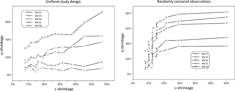
Relationship between η- and ε-shrinkage was studies using model 7. First, rich datasets were simulated (number of observations = 25). Then, sparse datasets were created by censoring observations within subjects either randomly or uniformly (same observation deleted for all subjects), keeping the total number of observations the same for all subjects. This procedure was repeated until two observations per subject remained. For each dataset, EBEs were estimated using the true model and true parameter estimates. η- and ε-shrinkage were calculated and inspected for relationships.
RESULTS
In general, in the absence of shrinkage, all EBE-based diagnostics are powerful model evaluation tools. These diagnostics separate different sources of variability, thus graphs become easier to interpret. However, in the presence of shrinkage, all the discussed diagnostics begin losing their informativeness and could potentially become misleading as indicated in our detailed evaluation of (1) consequences of η-shrinkage, (2) consequences of ε-shrinkage, and (3) relationship between η- and ε-shrinkage.
Consequences of η-Shrinkage
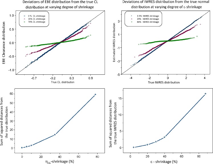
EBEs may, in addition to shrinkage, show non-normal distribution even when the true underlying η distribution is normal. A pattern of increasing deviations from normality in the qq-plot with increasing shrinkage, exemplified in Fig. 1 (left panels) for EBE of ηCL, was evident for all parameters of the studied model (model 4). The larger the shrinkage, the larger are the observed deviations from normality.
Fig. 1.
Deviation of empirical Bayes estimates (EBE) and individual weighted residual (IWRES) distribution from normality due to η- and ε-shrinkage, respectively, shown as a qq-plot (upper panels) and sum of squared distances from the true distributions (lower panels). This is a representative example of three simulations. EBE and IWRES were estimated using the true model
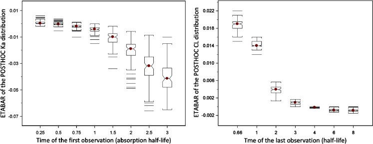
As a result of asymmetric η-shrinkage, mean values of EBEs (“ETABAR”) may be significantly different from zero, even for a correctly specified model. The relationship between ETABAR for ηka and ηCL distributions and the time of the first or last sample, respectively, is shown in Fig. 2. For ηka, when the first sample is taken early enough, i.e., informative on this parameter, ETABAR is close to zero, as expected. If the first sample is taken later in time, this sample is not particularly informative for individuals that have fast absorption because their absorption process is essentially complete by that time, but it will still be informative for individuals that have slow absorption; thus, shrinkage is expected to happen mainly for individuals with high ka values, which leads to asymmetric shrinkage resulting in ETABAR values significantly different from zero. A similar phenomenon is evident for the ηCL EBE distribution (right panel of Fig. 2).
Fig. 2.
Dependence of ETABAR on the time of the first and last sample for η ka and η CL distribution, respectively. Deviations of ETABAR from zero is a result of asymmetric empirical Bayes estimates shrinkage
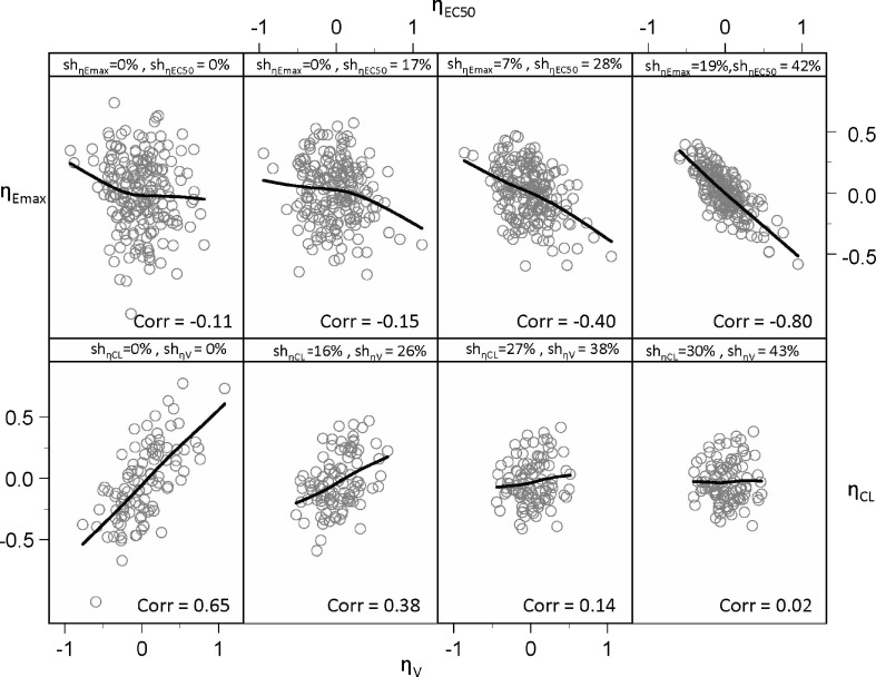
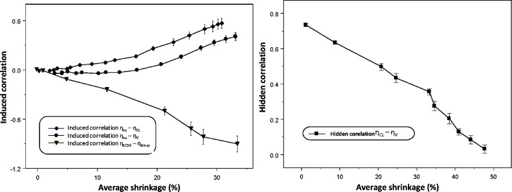
When EBEs are used for inspections for parameter correlations, they can indicate correlation when correlation truly does not exist (upper panel of Fig. 3), and oppositely, correlation when truly present would sometimes not been detected by EBEs (lower panel of Fig. 3). The upper-left corner and lower-left corner panels of Fig. 3 represent the true parameter relationships, while other panels show relationships based on the EBEs estimated under the true model for different study designs. As Fig. 4 indicates, commonly induced correlations include those between ηEC50 ∼ ηEmax and ηka ∼ ηV. The quantitative relationship between shrinkage extent and informativeness of these plots is shown in Fig. 4. Both phenomena, induced and hidden correlations, become apparent when shrinkage is higher than 20–30%.
Fig. 3.
Empirical Bayes estimates (EBE) versus EBE plot indicating parameter correlation due to η-shrinkage when correlation is not truly present (upper panel) and hiding parameter correlation when correlation is truly present (lower panel)
Fig. 4.
Left panel: relationship between (induced) correlation between η Emax and η EC50, η ka–η V and η ka–η CL, and η-shrinkage. Right panel: disappearance of correlation between empirical Bayes estimates with increased shrinkage. The average of the shrinkage in two studied parameters (e.g., η Emax and η EC50) is shown on the x-axes. Each symbol represents mean (SE) based on ten simulation–estimation procedures
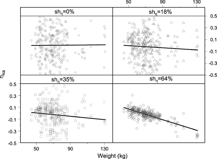
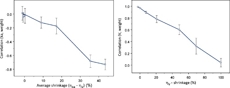
Similarly, when EBEs are used for a search of significant covariates, they can obscure relationships, show distorted shape, or even in certain circumstances falsely indicate relationship, when relationship truly does not exist (Figs. 5 and 6). The left panel of Fig. 6 shows falsely induced relationship between ηka and weight, when the true covariate relationship was between volume and weight. The right panel of Fig. 6 shows how an existing relationship between weight and ηV is less evident, the higher the shrinkage in ηV. The observed pattern appears due to induced correlation between ηka and ηV.
Fig. 5.
Empirical Bayes estimates versus covariate plot indicating parameter-covariate relationship due to η-shrinkage when relationship is not truly present
Fig. 6.
Relationship between shrinkage extent and induced covariate (left panel) and hidden covariate relationship (right panel). The average of the η ka- and η V-shrinkage is shown on the x-axes of the left panel
Consequences of ε-Shrinkage
The IWRES distribution may in the presence of ε-shrinkage show non-normal distribution even when the underlying model is correct (Fig. 1, right panel).
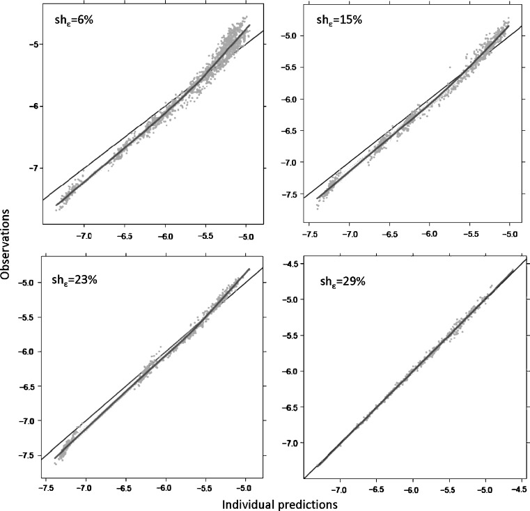
The power of IPREDs to detect model misspecification is reduced in the presence of ε-shrinkage. Figure 7 shows the DV versus IPRED diagnostic when a misspecified model (zero order absorption, model 5) was applied to data simulated with first order absorption (model 5) in two scenarios: with rich data resulting with low ε-shrinkage and with sparse data resulting in high η- and ε-shrinkage. When ε-shrinkage is low, the plot clearly indicates the model misspecification; however, when shrinkage is substantial, signs of model misspecification are absent, and the plot indicates a perfect fit. Similar phenomena were observed with all other scenarios tested. Already, at the ε-shrinkage extent of 20–30%, it was hard to visually detect model misspecification.
Fig. 7.
Individual prediction versus dependent variable plot for detection of structural model misspecification
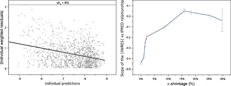
The power of IWRES to detect residual model misspecification diminishes with an increase in ε-shrinkage. Figure 8 (left panel) shows IWRES diagnostics produced based on misspecified model (proportional residual error only) fitted to the data simulated with the model that had combined error model (additive + proportional residual error). A quantitative relationship between ε-shrinkage and model misspecification indication, expressed as the slope of the regression line for |IWRES| versus IPRED, is shown in Fig. 8 (right panel).
Fig. 8.
Power of individual weighted residual (|IWRES|) versus individual prediction (IPRED) to detect residual model misspecification. In absence of shrinkage, the regression line of |IWRES| versus IPRED clearly indicates residual model misspecification (left panel). With increased shrinkage, the slope of the regression line is diminishing (right panel)
Relationship between η- and ε-Shrinkage
Relationships between η- and ε-shrinkage are shown in Fig. 9. As expected, these two terms are positively correlated. The shape of this relationship is however different for different study designs.
Fig. 9.
Relationship between η- and ε-shrinkage under different study designs
DISCUSSION
In this paper, we have evaluated the usefulness of EBE-based diagnostics in different circumstances and their dependencies on the information content in the datasets. These diagnostics are powerful when the individual’s data provide a substantial amount of information on the model parameters. However, with decreased information content per individual, these diagnostics become not only uninformative but potentially also misleading. The EBE-based diagnosis is a central part of the model building process, but if a modeler would accept such diagnostics without considering shrinkage, it may impede decision-making, increase time for data analysis, decrease trust in adequate models, and accept inappropriate models.
Although it is difficult to give a rule of thumb at what shrinkage extent diagnostics becomes misleading, we observed in our examples that already at a level of 20–30% for both, η- and ε-shrinkage, EBE-based diagnostics generally lost their power, and false indications started to appear. Therefore, it seems rational to provide values for shrinkage whenever EBE-based diagnostics are used for communicating model quality. It is important to clarify that all mentioned patterns are associated with the graphical diagnostics solely. When both models were tested directly in NONMEM, correct and misspecified, the correct model would be selected for every example, based on standard model building procedures using the objective function values. Thus, significant shrinkage in most of the cases does not indicate any problem with the dataset or with the model; it only affects the diagnostics based on EBE. Thus, whenever shrinkage is present, a model building process involving more direct testing and less or no reliance on EBE-based diagnostics should be used. Additionally, other types of diagnostics ought to be used in these cases, for example simulation-based diagnostic (10) or conditional weighted residuals (14).
An interesting finding was that EBEs may in the presence of shrinkage indicate false relationships or hide true relationships when used for covariate screening. Here, this was a consequence of the induced correlation between two parameters, ηka and ηV. (in general, sign of such an induced correlation may depend on the design). This finding is of special interest when EBEs are used for selection of covariates that will be further tested in the model for their significance. If only certain parameters are screened for covariates, it may happen that EBEs would indicate false parameter-covariate relationships, which may even turn out to be significant when tested directly in the model, while the covariate was truly related to other parameter. Therefore, whenever this is the case (i.e., single parameter is screened for covariate relationships and a certain covariate appears to be significant), the modeler should also test the relationship between the significant covariate and other parameters in order to determine the appropriate relationship.
We have observed that η- and ε-shrinkages are correlated, which is intuitive. However, while η-shrinkage may appear substantial even when observations per subject are numerous, ε-shrinkage remains low in these circumstances. ε-Shrinkage becomes substantial when the number of observations is equal or less than the number of random effects. As a general principle, the lower the residual variability, the more informative are observations, and the lower will the η-shrinkage be. Also, as a general principle, a higher number of between-subject random effect and higher variability in these will lead to a higher flexibility in the individual model to approach to observed values and therefore lead to higher ε-shrinkage.
We have so far only discussed shrinkage magnitudes between zero and one. Based on theoretical considerations, η- and ε-shrinkage should, in the absence of model misspecification, be positive (15). Indeed, whenever the shrinkage was computed under the correct model, shrinkage values were in this range. For a number of scenarios when data were simulated and model parameters re-estimated with misspecifications of the parameter distribution, shrinkage was non-negative. However, shrinkage may also take negative values in certain circumstances; we found negative shrinkage in some real data examples, typically with rich data and a small number of subjects. Also, in situations where a parameter variance is fixed to a lower value than the true value, negative shrinkage may occur. Thus, negative shrinkage may be a useful signal for possible model misspecification.
This exercise was performed on simulation examples, and one can argue that such scenarios would not occur often in model building processes using data from real clinical trials. However, when inspecting 29 published PK and PD models, we identified that shrinkage was present in all of them (Table II). Substantial shrinkage is often present in PD parameters and PK parameters describing absorption and distribution. Even the most well-informed parameter, clearance (CL), showed shrinkage above 20% in about one third of the PK studies. A large number of observations do not guarantee the absence of η-shrinkage as it can occur even in cases when the number of samples is as large as 20 observations per individual. This is simply because the studies are not designed to provide perfect information on all model parameters. In this work, we explored implications of EBE shrinkage for model diagnostics. However, EBEs are also used in other aspects of non-linear mixed effect analysis, for example, in FOCE, sequential PK-PD analysis or nonparametric estimation in NONMEM (14,16,17). Shrinkage would affect these estimation procedures too; however, this is outside the scope of the present investigation.
Table II.
Summary of the 29 Models Used to Assess the Shrinkage in Published Models with Real Datasets
| Model | Type | Number of obs | Number of ind | Number of obs/ind (average) | Number of θ | Number of η | Shrinkage (min) | Shrinkage (max) | Shrinkage CL |
|---|---|---|---|---|---|---|---|---|---|
| CdA (18) | PK | 1,102 | 161 | 6.84 | 12 | 7 | 6.66 | 84.17 | 6.66 |
| Pefloxacin (19) | PK | 337 | 74 | 4.55 | 2 | 2 | 5.16 | 37.68 | 5.16 |
| Glibenclamide lag time (20) | PK | 287 | 8 | 35.88 | 9 | 5 | −4.38 | 13.14 | −4.38 |
| Glibenclamide transit (21) | PK | 287 | 8 | 35.88 | 10 | 7 | −4.05 | 12.72 | −4.05 |
| Desmopressin kid lag time (22) | PK | 139 | 72 | 1.93 | 5 | 4 | 5.91 | 42.35 | 5.91 |
| Desmopressin kid transit (22) | PK | 139 | 72 | 1.93 | 6 | 5 | 8.61 | 66.97 | 8.61 |
| Desmopressin adult lag time (22) | PK | 373 | 28 | 13.32 | 5 | 4 | 2.17 | 5.83 | 2.36 |
| Desmopressin adult transit (22) | PK | 373 | 28 | 13.32 | 6 | 7 | 0.73 | 51.21 | 0.99 |
| Desmopressin joint lag time (22) | PK | 512 | 100 | 5.12 | 10 | 4 | 11.51 | 32.15 | 11.51 |
| Desmopressin joint transit (22) | PK | 512 | 100 | 5.12 | 8 | 6 | 13.80 | 49.47 | 13.80 |
| Levosimendan (23) | PK | 359 | 24 | 14.96 | 5 | 4 | 0.95 | 33.41 | 0.95 |
| Antibody Atm-027 (24) | PK | 413 | 14 | 29.50 | 8 | 4 | −1.39 | 17.37 | 1.26 |
| Moxonidine lag time (25) | PK | 1,022 | 74 | 13.81 | 6 | 6 | 17.76 | 54.18 | 32.38 |
| Moxonidine transit (21) | PK | 1,022 | 74 | 13.81 | 7 | 9 | 14.33 | 97.10 | 36.62 |
| Gefitinib (26) | PK | 705 | 34 | 20.74 | 7 | 5 | −0.58 | 5.55 | −0.35 |
| Melagatran (27) | PK | 3,595 | 596 | 6.03 | 8 | 3 | 12.63 | 38.03 | 12.63 |
| Pyrazinamide (28) | PK | 3,092 | 227 | 13.62 | 10 | 6 | 13.79 | 85.82 | 16.31 |
| Prazosin (29,30) | PK | 887 | 64 | 13.86 | 8 | 8 | 14.44 | 56.25 | 44.86 |
| Antibody X | PK | 559 | 70 | 7.99 | 6 | 4 | 16.85 | 43.56 | 16.85 |
| Voriconazole (31) | PK | 1,274 | 83 | 15.35 | 11 | 8 | 2.04 | 92.58 | 71.77 |
| Tobramycin (32) | PK | 322 | 97 | 3.32 | 5 | 1 | 8.46 | 90.77 | 8.46 |
| Levodopa (33) | PD | 851 | 19 | 44.79 | 7 | 7 | −1.80 | 38.64 | NA |
| Digoxin (34) | PD | 787 | 225 | 3.50 | 5 | 2 | 7.10 | 71.94 | NA |
| CdA (35) | PD | 341 | 59 | 5.78 | 5 | 3 | 2.44 | 25.46 | NA |
| Docetaxel (36) | PD | 3,549 | 636 | 5.58 | 11 | 4 | 18.29 | 46.64 | NA |
| Moxonidine (blood pressure; 37) | PD | 1,942 | 97 | 20.02 | 8 | 3 | 3.72 | 34.94 | NA |
| Moxonidine (heart rate; 37) | PD | 1,944 | 97 | 20.04 | 5 | 2 | 3.81 | 31.73 | NA |
| Tesaglitazar (FPG; 38) | PD | 4,035 | 412 | 9.79 | 9 | 4 | 6.26 | 38.26 | NA |
| Tesaglitazar (HbA1C measurements; 39) | PD | 4,663 | 412 | 11.32 | 13 | 5 | 1.54 | 42.39 |
The number of observations (dependent variables), individuals, and random effects are summarized as well as maximum and minimum η-shrinkage values. Please see referenced articles for further information
obs observations, ind individuals, NA not applicable, PK pharmacokinetic, PD pharmacodynamic, FPG fasting plasma glucose, CL clearance
In conclusion, when shrinkage is higher than about 20–30%, EBE-based diagnostics lack informativeness and may be misleading. Therefore, it is desirable to report the extent of ε- and η-shrinkage to assess the relevance of diagnostics employing EBEs, IPRED, and IWRES. When shrinkage is high, other diagnostics and more direct population model estimation need to be employed in model building and evaluation.
Acknowledgements
The authors would like to thank Dr. Siv Jönsson for valuable comments on the manuscript, Paul Baverel for his help with reviewing shrinkage in real models and datasets, and the anonymous reviewers for their valuable comments on the manuscript.
References
- 1.Williams PJ, Ette EI, editors. Pharmacometrics: the science of quantitative pharmacology. New York: Wiley; 2007. [Google Scholar]
- 2.Ette EI, Ludden TM. Population pharmacokinetic modeling: the importance of informative graphics. Pharm Res. 1995;12:1845–1855. doi: 10.1023/A:1016215116835. [DOI] [PubMed] [Google Scholar]
- 3.Jonsson EN, Karlsson MO. Xpose—an S-PLUS based population pharmacokinetic/pharmacodynamic model building aid for NONMEM. Comput Methods Programs Biomed. 1999;58:51–64. doi: 10.1016/S0169-2607(98)00067-4. [DOI] [PubMed] [Google Scholar]
- 4.FDA . Guidance for industry, population pharmacokinetics. Washington, DC: US Department of Health and Human Services; 1999. [Google Scholar]
- 5.Wade JR, Edholm M, Salmonson T. A guide for reporting the results of population pharmacokinetic analyses: A Swedish perspective. AAPS J. 2005;7(2):45. doi: 10.1208/aapsj070245. [DOI] [PMC free article] [PubMed] [Google Scholar]
- 6.Bhattaram VA, Booth BP, Ramchandani RP, Beasley BN, Wang Y, Tandon V, Duan JZ, Baweja RK, Marroum PJ, Uppoor RS, Rahman NA, Sahajwalla CG, Powell JR, Mehta MU, Gobburu JV. Impact of pharmacometrics on drug approval and labeling decisions: a survey of 42 new drug applications. AAPS J. 2005;7:E503–E512. doi: 10.1208/aapsj070351. [DOI] [PMC free article] [PubMed] [Google Scholar]
- 7.Davidian M, Giltinan DM. Nonlinear models for repeated measurement data. London: Chapman & Hall/CRC; 1995. [Google Scholar]
- 8.Sheiner LB, Beal S, Rosenberg B, Marathe VV. Forecasting individual pharmacokinetics. Clin Pharmacol Ther. 1979;26:294–305. doi: 10.1002/cpt1979263294. [DOI] [PubMed] [Google Scholar]
- 9.Sheiner LB, Beal SL. Bayesian individualization of pharmacokinetics: simple implementation and comparison with non-Bayesian methods. J Pharm Sci. 1982;71:1344–1348. doi: 10.1002/jps.2600711209. [DOI] [PubMed] [Google Scholar]
- 10.Karlsson MO, Savic RM. Diagnosing model diagnostics. Clin Pharmacol Ther. 2007;82:17–20. doi: 10.1038/sj.clpt.6100241. [DOI] [PubMed] [Google Scholar]
- 11.Wang Y. Derivation of various NONMEM estimation methods. J Pharmacokinet Pharmacodyn. 2007;34:575–593. doi: 10.1007/s10928-007-9060-6. [DOI] [PubMed] [Google Scholar]
- 12.Beal SL, Sheiner LB, Boeckmann AJ. NONMEM users guides. Ellicott City, MD: Icon Development Solutions; 1989–2006.
- 13.Jonsson EN, Karlsson MO. Automated covariate model building within NONMEM. Pharm Res. 1998;15:1463–1468. doi: 10.1023/A:1011970125687. [DOI] [PubMed] [Google Scholar]
- 14.Hooker AC, Staatz CE, Karlsson MO. Conditional weighted residuals (CWRES): a model diagnostic for the FOCE method. Pharm Res. 2007;24:2187–2197. doi: 10.1007/s11095-007-9361-x. [DOI] [PubMed] [Google Scholar]
- 15.Verbeke G, Molenberghs G. Linear mixed models for longitudinal data. New York: Springer; 2000. pp. 80–81. [Google Scholar]
- 16.Zhang L, Beal SL, Sheiner LB. Simultaneous vs. sequential analysis for population PK/PD data I: best-case performance. J Pharmacokinet Pharmacodyn. 2003;30:387–404. doi: 10.1023/B:JOPA.0000012998.04442.1f. [DOI] [PubMed] [Google Scholar]
- 17.Savic RM, Kjellsson MC, Karlsson MO. Evaluation of the nonparametric estimation method in NONMEM VI. Eur J Pharm Sci. 2009;37:27–35. doi: 10.1016/j.ejps.2008.12.014. [DOI] [PubMed] [Google Scholar]
- 18.Lindemalm S, Savic RM, Karlsson MO, Juliusson G, Liliemark J, Albertioni F. Application of population pharmacokinetics to cladribine. BMC Pharmacol. 2005;5:4. doi: 10.1186/1471-2210-5-4. [DOI] [PMC free article] [PubMed] [Google Scholar]
- 19.Bruno R, Iliadis MC, Lacarelle B, Cosson V, Mandema JW, Le Roux Y, Montay G, Durand A, Ballereau M, Alasia M, et al. Evaluation of Bayesian estimation in comparison to NONMEM for population pharmacokinetic data analysis: application to pefloxacin in intensive care unit patients. J Pharmacokinet Biopharm. 1992;20:653–669. doi: 10.1007/BF01064424. [DOI] [PubMed] [Google Scholar]
- 20.Rydberg T, Jonsson A, Karlsson MO, Melander A. Concentration-effect relations of glibenclamide and its active metabolites in man: modelling of pharmacokinetics and pharmacodynamics. Br J Clin Pharmacol. 1997;43:373–381. doi: 10.1111/j.1365-2125.1997.00571.x. [DOI] [PMC free article] [PubMed] [Google Scholar]
- 21.Savic RM, Jonker DM, Kerbusch T, Karlsson MO. Implementation of a transit compartment model for describing drug absorption in pharmacokinetic studies. J Pharmacokinet Pharmacodyn. 2007;34:711–726. doi: 10.1007/s10928-007-9066-0. [DOI] [PubMed] [Google Scholar]
- 22.Osterberg O, Savic RM, Karlsson MO, Simonsson US, Norgaard JP, Walle JV, Agerso H. Pharmacokinetics of desmopressin administrated as an oral lyophilisate dosage form in children with primary nocturnal enuresis and healthy adults. J Clin Pharmacol. 2006;46:1204–1211. doi: 10.1177/0091270006291838. [DOI] [PubMed] [Google Scholar]
- 23.Jonsson EN, Antila S, McFadyen L, Lehtonen L, Karlsson MO. Population pharmacokinetics of levosimendan in patients with congestive heart failure. Br J Clin Pharmacol. 2003;55:544–551. doi: 10.1046/j.1365-2125.2003.01778.x. [DOI] [PMC free article] [PubMed] [Google Scholar]
- 24.Zingmark PH, Edenius C, Karlsson MO. Pharmacokinetic/pharmacodynamic models for the depletion of Vbeta5.2/5.3 T cells by the monoclonal antibody ATM-027 in patients with multiple sclerosis, as measured by FACS. Br J Clin Pharmacol. 2004;58:378–389. doi: 10.1111/j.1365-2125.2004.02177.x. [DOI] [PMC free article] [PubMed] [Google Scholar]
- 25.Karlsson MO, Jonsson EN, Wiltse CG, Wade JR. Assumption testing in population pharmacokinetic models: illustrated with an analysis of moxonidine data from congestive heart failure patients. J Pharmacokinet Biopharm. 1998;26:207–246. doi: 10.1023/A:1020561807903. [DOI] [PubMed] [Google Scholar]
- 26.Li J, Karlsson MO, Brahmer J, Spitz A, Zhao M, Hidalgo M, Baker SD. CYP3A phenotyping approach to predict systemic exposure to EGFR tyrosine kinase inhibitors. J Natl Cancer Inst. 2006;98:1714–1723. doi: 10.1093/jnci/djj466. [DOI] [PubMed] [Google Scholar]
- 27.Cullberg M, Eriksson UG, Wahlander K, Eriksson H, Schulman S, Karlsson MO. Pharmacokinetics of ximelagatran and relationship to clinical response in acute deep vein thrombosis. Clin Pharmacol Ther. 2005;77:279–290. doi: 10.1016/j.clpt.2004.11.001. [DOI] [PubMed] [Google Scholar]
- 28.Wilkins JJ, Langdon G, McIlleron H, Pillai GC, Smith PJ, Simonsson US. Variability in the population pharmacokinetics of pyrazinamide in South African tuberculosis patients. Eur J Clin Pharmacol. 2006;62:727–735. doi: 10.1007/s00228-006-0141-z. [DOI] [PubMed] [Google Scholar]
- 29.Karlsson MO, Sheiner LB. The importance of modeling interoccasion variability in population pharmacokinetic analyses. J Pharmacokinet Biopharm. 1993;21:735–750. doi: 10.1007/BF01113502. [DOI] [PubMed] [Google Scholar]
- 30.Mandema JW, Verotta D, Sheiner LB. Building population pharmacokinetic–pharmacodynamic models. I. Models for covariate effects. J Pharmacokinet Biopharm. 1992;20:511–528. doi: 10.1007/BF01061469. [DOI] [PubMed] [Google Scholar]
- 31.Karlsson MO, Lutsar I, Milligan PA. Population pharmacokinetic analysis of voriconazole plasma concentration data from pediatric studies. Antimicrob Agents Chemother. 2009;53:935–944. doi: 10.1128/AAC.00751-08. [DOI] [PMC free article] [PubMed] [Google Scholar]
- 32.Aarons L, Vozeh S, Wenk M, Weiss P, Follath F. Population pharmacokinetics of tobramycin. Br J Clin Pharmacol. 1989;28:305–314. doi: 10.1111/j.1365-2125.1989.tb05431.x. [DOI] [PMC free article] [PubMed] [Google Scholar]
- 33.Troconiz IF, Naukkarinen TH, Ruottinen HM, Rinne UK, Gordin A, Karlsson MO. Population pharmacodynamic modeling of levodopa in patients with Parkinson’s disease receiving entacapone. Clin Pharmacol Ther. 1998;64:106–116. doi: 10.1016/S0009-9236(98)90028-5. [DOI] [PubMed] [Google Scholar]
- 34.Hornestam B, Jerling M, Karlsson MO, Held P. Intravenously administered digoxin in patients with acute atrial fibrillation: a population pharmacokinetic/pharmacodynamic analysis based on the digitalis in acute atrial fibrillation trial. Eur J Clin Pharmacol. 2003;58:747–755. doi: 10.1007/s00228-002-0553-3. [DOI] [PubMed] [Google Scholar]
- 35.Lindemalm S, Liliemark J, Gruber A, Eriksson S, Karlsson MO, Wang Y, Albertioni F. Comparison of cytotoxicity of 2-chloro-2′-arabino-fluoro-2′-deoxyadenosine (clofarabine) with cladribine in mononuclear cells from patients with acute myeloid and chronic lymphocytic leukemia. Haematologica. 2003;88:324–332. [PubMed] [Google Scholar]
- 36.Friberg LE, Henningsson A, Maas H, Nguyen L, Karlsson MO. Model of chemotherapy-induced myelosuppression with parameter consistency across drugs. J Clin Oncol. 2002;20:4713–4721. doi: 10.1200/JCO.2002.02.140. [DOI] [PubMed] [Google Scholar]
- 37.Brynne L, McNay JL, Schaefer HG, Swedberg K, Wiltse CG, Karlsson MO. Pharmacodynamic models for the cardiovascular effects of moxonidine in patients with congestive heart failure. Br J Clin Pharmacol. 2001;51:35–43. doi: 10.1046/j.1365-2125.2001.01320.x. [DOI] [PMC free article] [PubMed] [Google Scholar]
- 38.Hamren B, Ericsson H, Samuelsson O, Karlsson MO. Mechanistic modelling of tesaglitazar pharmacokinetic data in subjects with various degrees of renal function—evidence of interconversion. Br J Clin Pharmacol. 2008;65:855–863. doi: 10.1111/j.1365-2125.2008.03110.x. [DOI] [PMC free article] [PubMed] [Google Scholar]
- 39.Hamren B, Bjork E, Sunzel M, Karlsson M. Models for plasma glucose, HbA1c, and hemoglobin interrelationships in patients with type 2 diabetes following tesaglitazar treatment. Clin Pharmacol Ther. 2008;84(2):228–235. doi: 10.1038/clpt.2008.2. [DOI] [PubMed] [Google Scholar]


