

Abstract
Finding the dynamics of an entire macromolecule is a complex problem as the model-free parameter values are intricately linked to the Brownian rotational diffusion of the molecule, mathematically through the autocorrelation function of the motion and statistically through model selection. The solution to this problem was formulated using set theory as an element of the universal set  —the union of all model-free spaces (d’Auvergne EJ and Gooley PR (2007) Mol BioSyst 3(7), 483–494). The current procedure commonly used to find the universal solution is to initially estimate the diffusion tensor parameters, to optimise the model-free parameters of numerous models, and then to choose the best model via model selection. The global model is then optimised and the procedure repeated until convergence. In this paper a new methodology is presented which takes a different approach to this diffusion seeded model-free paradigm. Rather than starting with the diffusion tensor this iterative protocol begins by optimising the model-free parameters in the absence of any global model parameters, selecting between all the model-free models, and finally optimising the diffusion tensor. The new model-free optimisation protocol will be validated using synthetic data from Schurr JM et al. (1994) J Magn Reson B 105(3), 211–224 and the relaxation data of the bacteriorhodopsin (1–36)BR fragment from Orekhov VY (1999) J Biomol NMR 14(4), 345–356. To demonstrate the importance of this new procedure the NMR relaxation data of the Olfactory Marker Protein (OMP) of Gitti R et al. (2005) Biochem 44(28), 9673–9679 is reanalysed. The result is that the dynamics for certain secondary structural elements is very different from those originally reported.
Electronic supplementary material
The online version of this article (doi:10.1007/s10858-007-9213-3) contains supplementary material, which is available to authorized users.
Keywords: Brownian rotational diffusion, Model-free analysis, Modelling, Molecular motion, NMR relaxation, Optimisation
Introduction
NMR is a powerful tool for probing the fast internal motions of macromolecules on the picosecond to nanosecond timescales. By collecting NMR relaxation data, specifically the R1 and R2 relaxation rates together with the steady-state NOE, information about the motions of individual bond vectors within the molecule can be gathered. Interpreting these raw numbers by themselves to create a cohesive dynamic description of the molecule is difficult. Therefore a number of theories exist to interpret these data. The most commonly used tool is model-free analysis (Lipari and Szabo 1982a, b; Clore et al. 1990a).
By parametric restriction of the original model-free equations of Lipari and Szabo (1982a, b) and the extension by Clore et al. (1990b) a large number of model-free mathematical models were constructed in the preceding paper (d’Auvergne and Gooley 2007a) which, henceforth, shall be referred to as Paper I. These models were labelled from m0 to m9 (Models 1.0–1.9 of Paper I). By assuming each spin system tumbles independently the overall rotational diffusion of each bond vector can be approximated by a separate correlation time, the local τm (Barbato et al. 1992; Schurr et al. 1994). The addition of this parameter creates a new set of model-free models which were labelled tm0 to tm9 in Paper I. NMR relaxation is influenced not by the correlation function C(τ) of the motions of the XH bond but by the power spectral density function J(ω), a quantity which is related to the correlation function via Fourier transform. Numerically stabilised forms of both the original and extended model-free spectral density functions are presented in Equations (2) and (3) of Paper I.
In this paper the optimisation of the global model  which consists of both the Brownian rotational diffusion tensor of the molecule and the internal model-free motions of individual bond vectors, will be studied. The entirety of the complex model-free problem, in which the motions of each spin system are both mathematically and statistically dependent on the diffusion tensor and vice versa, can be formulated using set theory (d’Auvergne and Gooley 2007b). Its solution can be derived as an element of the universal set
  the union of the diverse model-free parameter spaces
  Each set
  is constructed from the union of the model-free models
  for all spin systems and the diffusion parameter set
  A single parameter gain or loss on a single spin system shifts optimisation to a different space
  The solution within the universal set
  which for simplicity will be referenced as the universal solution
  can be formulated as (d’Auvergne and Gooley 2007b)
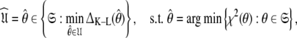 |
1 |
where  is the optimised parameter vector of the space
  is the Kullback–Leibler discrepancy (Kullback and Leibler 1951), and χ2(θ) is the chi-squared function which is minimised. The equation consists of two parts, the first component belongs to the statistical field of model selection (Akaike 1973; Schwarz 1978; Linhart and Zucchini 1986; Burnham and Anderson 1998; Zucchini 2000; d’Auvergne and Gooley 2003) whereas the second belongs to the mathematical field of optimisation (Nocedal and Wright 1999; d’Auvergne and Gooley 2007a).
Ever since the original model-free publications (Lipari and Szabo 1982a, b) the model-free problem has been tackled by first finding an initial estimate of the diffusion tensor and then determining the model-free dynamics of the system. This concept, which for brevity will be called the diffusion seeded model-free paradigm, is now highly evolved and much theory has emerged to improve this path to the solution  The technique can, at times, suffer from its rigidity assumption (Orekhov et al. 1995, 1999a, b; Korzhnev et al. 1997; d’Auvergne and Gooley 2007b). Here a different approach is proposed for finding the universal solution
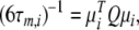
  of the extremely complex, convoluted model-free optimisation and modelling problem. This new model-free optimisation protocol incorporates the ideas of the local τm model-free model (Barbato et al. 1992; Schurr et al. 1994) and the optimisation of the diffusion tensor using information from these models, analogously to the linear least-squares fitting of the quadric model (Brüschweiler et al. 1995; Lee et al. 1997). The quadric model is a methodology for determining the diffusion tensor from the local τm parameter together with the orientation of the XH bond represented by the unit vector μi. A local τm value is obtained for each spin i by optimising tm2 and then the τm,i values are approximated using the quadric model
 |
2 |
where the eigenvalues of the matrix Q are defined as  and
and  The diffusion tensor is then found by linear least-squares fitting.
The new protocol follows the lead of Butterwick et al. (2004) whereby the diffusion seeded model-free paradigm was reversed. Rather than starting with an initial estimate of the global diffusion tensor from the set  the protocol starts with the model-free parameters from
  The first step of the protocol is the reduced spectral density mapping of Farrow et al. (1995). As Rex has been eliminated from the analysis, three model-free models corresponding to tm1, tm2, and tm5 are employed. The model-free parameters are optimised using the reduced spectral density values and the best model is selected using F-tests. The spherical, spheroidal, and ellipsoidal diffusion tensors are obtained by linear least-squares fitting of the quadric model of Eq. 2 using the local τm values (Brüschweiler et al. 1995; Lee et al. 1997). The best diffusion model is selected via F-tests and refined by iterative elimination of spin systems with high chi-squared values. This tensor is used to calculate local τm values for each spin system, approximating the multiexponential sum of the Brownian rotational diffusion correlation function with a single exponential (Woessner 1962; d’Auvergne 2006), using the quadric model of Eq. 2. In the final step of the protocol these τm values are fixed and m1, m2, and m5 (Models 1.1, 1.2, and 1.5 of Paper I) are optimised and the best model-free model selected using F-tests.
The new model-free optimisation protocol utilises the core foundation of the Butterwick et al. (2004) protocol yet its divergent implementation is designed to solve Eq. 1 to find  Models tm0 to tm9 in which no global diffusion parameters exist are employed to significantly collapse the complexity of the problem. Model-free minimisation (Paper I), model elimination (d’Auvergne and Gooley 2006), and then AIC model selection (Akaike 1973; d’Auvergne and Gooley 2003) can be carried out in the absence of the influence of global parameters. By removing the local τm parameter and holding the model-free parameter values constant these models can then be used to optimise the diffusion parameters of
  Model-free optimisation, model elimination, AIC model selection, and optimisation of the global model
  is iterated until convergence. The iterations allow for sliding between different universes
  to enable the collapse of model complexity, to refine the diffusion tensor, and to find the solution within the universal set
  The last step is the AIC model selection between the different diffusion models. Because the AIC criterion approximates the Kullback–Leibler discrepancy which is central to the universal solution in Eq. 1 it was chosen for all three model selection steps over BIC model selection (Schwarz 1978; d’Auvergne and Gooley 2003; Chen et al. 2004). The new protocol avoids the problem of under-fitting whereby artificial motions appear (Schurr et al. 1994; Tjandra et al. 1996; Mandel et al. 1996; Luginbühl et al. 1997; Gagné. 1998; d’Auvergne and Gooley 2007b), avoids the problems involved in finding the initial diffusion tensor within
  including the decision of which bond vectors to utilise for the initial analysis using deviations from the average R2/R1 ratio and low NOE values (Kay et al. 1989; Clore et al. 1990a; Stone et al. 1992; Barbato et al. 1992; Tjandra et al. 1995a; d’Auvergne and Gooley 2007b), and avoids the problem of hidden internal nanosecond motions and the inability to slide between universes to get to
  (Orekhov et al. 1995, 1999a, b; Korzhnev et al. 1997; d’Auvergne and Gooley 2007b).
Methods
A new model-free optimisation protocol
The five diffusion models
Rather than pursuing the elemental idea whereby the universal solution  is sought by initially estimating the optimal parameters
  of the diffusion set
  and then using these estimates to determine the optimal parameter values
  and models
  of the model-free dynamics of the molecule (d’Auvergne and Gooley 2007b), the universal solution
  can also be found by applying the reverse of this logic. Initially the model-free parameter values
  and models
  can be determined by optimisation and model selection respectively. Finally, the parameters
  of the diffusion tensor
  can be optimised. To find the universal solution
  five categories of global model
  are constructed
 |
3.1 |
 |
3.2 |
 |
3.3 |
 |
3.4 |
 |
3.5 |
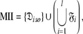
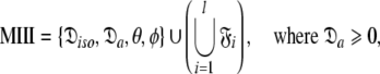
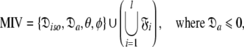
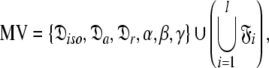
where l is the total number of spin systems used in the analysis and  is one of the model-free models m0 to m9 for spin system i.
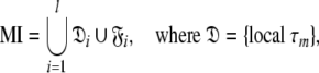
Model I (MI)—local τm
The value of the local τm is dependent on the geometry of the true diffusion tensor and the orientation of the XH bond vector (Barbato et al. 1992; Schurr et al. 1994). The MI diffusion model encompasses all the model-free models and not simply the single tm2 model which was used in Barbato et al. (1992) to study protein interdomain motions, in Schurr et al. (1994) to avoid artificial nanosecond motions when diffusion anisotropy is not taken into account, and in Bruschweiler et al. (1995) to determine the ellipsoidal diffusion tensor.
Although the introduction of model MI significantly increases the number of universes  where originally
 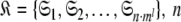 is the number of Brownian rotational diffusion models, m is the number of model-free models, and l is the number of spin systems, for the subset MI
  a complete collapse of the complexity of the global problem occurs. As no global parameters exist in these models the space
  can be broken into l independent components or spaces
  where i is spin system number. The spaces
  are synonymous with model-free models tm0 to tm9 defined in Paper I. The complexity reduces to
 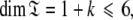 where 1 represents the single local τm parameter and k is the number of model-free parameters. Due to this dimensionality collecting six relaxation data sets at a minimum of two field strengths is essential. This drastic dissolution of complexity is key to solving the chicken-and-egg problem of the dual optimisation of the diffusion tensor and the model-free models.
To find the solution in MI, defined as the space  which minimises ΔK–L in Eq. 1 solely for the subset MI
  three simple steps are required. Firstly and separately for each spin system the parameters of model-free models tm0 to tm9 are optimised using Newton minimisation as described in Paper I. Failed models are then eliminated as described in d’Auvergne and Gooley (2006). The last step is to select between models tm0 to tm9 using AIC model selection to minimise the value of ΔK–L (d’Auvergne and Gooley 2003).
Model II (MII)—the sphere
This subset of models represents the diffusion as a sphere, or isotropic diffusion. The initial stage of optimisation involves setting the model-free models to those of MI but with the local τm parameter removed. The model-free parameter values, taken from MI, are then held constant while the single global diffusion parameter τm is optimised.
The space  which has now been isolated, although very close to the solution of Eq. 1 for the subset MII, may not actually be the space which minimises ΔK–L due to the approximate nature of model MI. Therefore a repetitive procedure, similar to the standard iterative methodology of the diffusion seeded model-free paradigm, is necessary to slide between universes
  to find the solution within the MII subset of
  By holding the optimised diffusion parameters constant model-free models m0 to m9 can be optimised. Failed models are then eliminated and the best model is selected using AIC model selection. Finally all diffusion and model-free parameters of the isolated space
  are optimised simultaneously. These steps are repeated until convergence—defined as identical model-free models (
 ) equal model-free and diffusion parameter values (
 ) and equal chi-squared values between iterations (χ2i = χ2i−1).
Model III (MIII)—the prolate spheroid
This subset represents the axially symmetric diffusion of the prolate spheroid. The procedure for optimising this model is the same as for MII except that the diffusion set  = {
= { } is minimised. In addition, the constraint
  is implemented to isolate the prolate spheroid subspace.
Model IV (MIV)—the oblate spheroid
This subset also represents axially symmetric diffusion but of the oblate spheroid. The technique is again the same as for MII except that the diffusion set  = {
= { } is minimised together with the constraint
  to isolate the oblate spheroid subspace.
Model V (MV)—the ellipsoid
This subset represents the rhombic or fully anisotropic diffusion of the ellipsoid. Applying the methodology used in MII, although using the diffusion set  = {
= { }, the solution for this subset MV
  can be found.
The universal solution 
Once all the global diffusion models have converged to satisfy Eq. 1 for their respective subsets of  the universal solution
  can be found by selecting between these global models using AIC model selection. If any of the models MI to MV have failed with diffusional correlation times shooting towards infinity or diffusion rates of zero these should be removed prior to model selection (d’Auvergne and Gooley 2006). Finally the parameter errors can be calculated by Monte Carlo simulation. The entirety of the new model-free optimisation protocol has been written into a single self contained relax script which is packaged with the program.
All optimisations of the model-free parameters, the diffusion parameters, or both sets simultaneously utilised the Newton line search algorithm combined with the backtracking step length selection technique (Nocedal and Wright 1999) and the GMW Hessian modification (Gill et al. 1981). The iterative Augmented Lagrangian algorithm was used to constrain the parameter values (Nocedal and Wright 1999). These techniques were investigated in Paper I.
Replication and extension of Schurr’s data
Due to truncation artefacts of using the R1, R2, and NOE values in Table 4 of Schurr et al. (1994) the relaxation data was regenerated from scratch. A PDB file of 12 NH bond vectors with the direction cosines between the NH bond vectors and the major axis of the prolate spheroid, 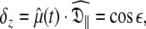 set to {1.00, 0.95, 0.85, 0.75, 0.65, 0.55, 0.45, 0.35, 0.25, 0.15, 0.05, 0.00} was created. Using the program relax relaxation data was generated for a prolate spheroid diffusion tensor with τm = 8.5 ns and
  = 1.3. Only dipolar relaxation was assumed as in Schurr et al. (1994). The bond length was not specified (ibid.) therefore a value of 1.02 Å was assumed. Model-free model m2 was chosen with S2 = 0.8 and τe = 50 ps. To use the new global optimisation protocol both 500 and 600 MHz data was generated. As a non-standard chi-squared statistic was used for minimisation (ibid.) errors needed to be generated so that the standard chi-squared formula could be used. To best reflect experimental errors values of 0.04 and 0.05 were used for the 600 and 500 MHz NOE respectively whereas 2% errors were used for all other data (d’Auvergne and Gooley 2003).
Dynamics of the bacteriorhodopsin fragment (1-36)BR
The R1, R2, and NOE relaxation data at 500, 600, and 750 MHz of the bacteriorhodopsin fragment (1-36)BR was extracted from the comments inside the PostScript file of the relaxation data figure from Orekhov et al. (1999a). For all optimisations a CSA value of −170 ppm and a bond length of 1.02 Å was used. All residues were included in the optimisation of the diffusion model MI. For the optimisation of the spherical diffusion tensor in model MII only residues 9 to 31 were selected.
The Olfactory Marker Protein
The R1, R2, and NOE values at both 600 and 800 MHz were taken from the supporting information. To mirror the original analysis values of −160 ppm and 1.02 Å were used for the CSA and amide NH bond length respectively. As the high precision NMR structures, refined using residual dipolar couplings (Wright et al. 2005), which were used in (Gitti et al. 2005) were not yet available from the PDB, the reanalysis of the relaxation data was carried out against the first model of the original NMR structure 1JYT of Baldisseri et al. (2002) as well as the 2.3 Å resolution X-ray crystallographic structure 1F35 of Smith et al. (2002).
Results and discussion
Three test systems
To test the new model-free optimisation protocol three test systems were examined. These include the data of Schurr et al. (1994) which explored the effect of NH bond vector orientations within the diffusion tensor frame when a too simplistic diffusion tensor is utilised; the bacteriorhodopsin fragment (1-36)BR data of Orekhov et al. (1999a) in which all residues experience nanosecond timescale motions; and the Olfactory Marker Protein data of Gitti et al. (2005) as a test case of a typical globular protein.
Artifacts induced by ignoring parsimony when selecting the diffusion model
Under-fitting
If the selected diffusion tensor is too simplistic then under-fitting occurs causing artefacts to appear in the dynamic description (Schurr et al. 1994; Tjandra et al. 1996). These artefacts are the manifestation of the bias introduced by not observing parsimony. When the Brownian diffusion of a molecule is that of a prolate spheroid and the internal motions are fast (assuming model m2), Schurr et al. (1994) demonstrated that the use of a spherical tensor together with the extended model-free formalism (using model m5) induces artificial sub-nanosecond timescale motions. This is best demonstrated in Table 4 (ibid.) which has been recalculated in Table S1 of the supplementary material.
To illustrate the second effect, revealed by Tjandra et al. (1996) whereby artificial Rex contributions appear across the protein, model m4 was minimised against the same data (Table S1). Again the spherical approximation of the diffusion tensor was utilised to force under-fitting. Comparing models m4 and m5 in Table S1 the diametrically opposing effects of the under-fitting of the two models are evident. Whereas the artificially slow sub-nanosecond motions appear perpendicular to the major axis of the prolate spheroid, the fictitious chemical exchange occurs when the bond vector is parallel to the major axis.
Occam’s razor
Using the new model-free optimisation protocol the tm2 model was chosen for all bond vectors when solving for the first step of the procedure, model MI. The S2 and τe values replicate the original internal motions whereas the local τm parameter over and under estimates the isotropic correlation time as the bond vector changes from parallel to perpendicular to the unique axis  Despite the triple exponential form of the rotational correlation function of the Brownian diffusion of a spheroid the single exponential of the local τm parameter adequately compensates. Table S2 of the supplementary material summarises the five global models (MI to MV) showing the total number of parameters, the global chi-squared value, and the AIC criteria. The AIC value of the oblate spheroid is very close to that of the prolate spheroid but even if this global model is used, the S2 and τe values are replicated to within 0.2% and 1% respectively (data not shown). Nevertheless the true prolate spheroid with model m2 used to create the data of Table 4 of Schurr et al. (1994) is easily isolated at the end with all parameters re-found to within machine precision. Thus, when using the new model-free optimisation protocol, both under-fitting and over-fitting are avoided and the principle of parsimony is closely adhered to.
Over-fitting
When too many parameters are included within the global model over-fitting occurs. This situation does not introduce bias and hence artifacts in the dynamics. If overly complex diffusion tensors are selected, and minimised properly, the diffusion parameters will take the values of the simpler, true model with the additional geometric parameters of  being statistically zero and the additional orientational parameters of
  being undefined. As Schurr’s data was noise-free this occurred for the ellipsoid diffusion tensor. A similar situation occurs if an overly complex model-free model is selected whereby the additional parameters take values which are insignificant. No statistically significant artefacts will appear if the diffusion tensor is over-fit, the worst consequence being the inclusion of additional noise into the model. Avoiding both under and over-fitting is purely the balancing of bias against variance (d’Auvergne and Gooley 2003).
Bacteriorhodopsin fragment (1-36)BR—testing the new optimisation protocol
Violation of the rigidity assumption
One of the major causes of failure of the diffusion seeded model-free protocol is the violation of the rigidity assumption. When the majority of the bond vectors of a molecule experience motions on the nanosecond timescale, local optimisation together with model selection combine to hide the slow motions and steer the final solution far from  An excellent test case representing a molecule in which the diffusion seeded model-free paradigm fails as all residues exhibit motions on the nanosecond timescale is the bacteriorhodopsin fragment (1-36)BR (Orekhov et al. 1999a). Applying the concept of estimating an initial diffusion tensor and using this as a starting point for model-free analysis causes the global correlation time to be underestimated. Subsequent minimisation of the model-free models to this global model will then hide the internal nanosecond motions (Korzhnev et al. 2001).
Avoiding the initial diffusion tensor estimate
In Orekhov et al. (1999a) a novel protocol was presented for avoiding the rigidity assumption and the need for an initial estimate diffusion tensor. Using this procedure, the global correlation time τm was found to be 5.77 ns and the average model-free parameter values were  and
and  ns. As the minimised chi-squared value was 120 and the number of parameters k was 66, the AIC value for this model is 252. To test the robustness of the new protocol in avoiding the hidden motion problem, the relaxation data of (1-36)BR was reanalysed. The final global models from Orekhov et al. (1999a) and that of the new model-free optimisation protocol are very similar. In fact, the parameters of the former are a subset of the latter. In addition to all residues having the parameters S2f, S2s, and τs the new protocol adds the parameter τf to the termini of the α-helix (residues 9, 10, 11, 12, 15, and 31) as well as the parameter Rex to residues 10 and 31. The averages of the common parameters have shifted to
  and
and  ns. In comparison with the AIC value of 252 for the isotropic model with all residues set to m5 (ibid.), the model of higher complexity determined by the new protocol is in fact more parsimonious (AIC = 238.09).
Reanalysis of the OMP relaxation data
To demonstrate the utility of the program relax and the application and consequences of new model-free optimisation protocol the NMR relaxation data of the Olfactory Marker Protein (OMP) from the original analysis of Gitti et al. (2005) has been reanalysed. This system was chosen as it was a recent analysis of the model-free dynamics of a protein system in which a number of the issues associated with the application of the diffusion seeded model-free paradigm are evident.
Global model MI—local τm
The local τm values of model MI are shown in Fig. 1. The trend of the values is similar to the R2/R1 ratio plot in Figure 2 of Gitti et al. (2005). Interestingly, the number of residues experiencing chemical exchange in this model is significantly lower than what was reported (ibid.). The chemical exchange is restricted to residues {26, 38, 44, 45, 46, 140} with values of {2.8±1.7, 6.6±0.7, 4.1±2.1, 1.4±0.9, 3.4±1.9, 3.4±1.4} respectively. The majority of the chemical exchange originally reported for residues 20 to 35 (helix α1) is not present and the entirety of the Rex values across residues 84 to 99 (Ω-loop 3) and residues 145 to 152 (β-hairpin loop 4) is also absent. Overlapping with this absence is an elevation of the local τm parameter in the three distinct yet spatially proximal regions of residues 19 to 50 (helix α1 and loop 1), 83 to 99, and 145 to 155.
Fig. 1.

The OMP local τm parameter values of global model MI after optimisation and AIC model selection. MI is the model whereby each residue of the protein is assumed to tumble independently and hence each residue is described by its own global correlation time, local τm. The Grace plot was created by relax
Iterative optimisation of global models MII to MV—finding the universal solution 
To slide from the initial position given by model MI to that of the universal solution, multiple iterations of optimising global models MII to MV are necessary (Fig. 2). Surprisingly, when sliding between different universes  en route to convergence the chi-squared value actually increases. For different macromolecules this is not always the case—during the optimisation of the bacteriorhodopsin (1-36)BR fragment the value decreased. This apparent inconsistency can simply be explained through the formulation of the universal solution in (1). Although each iteration minimises the chi-squared value, by contrast the overall iterative procedure minimises ΔK–L. The AIC plot in Fig. 2 demonstrates the decrease of the discrepancy across iterations. Since AIC = χ2 + 2k (d’Auvergne and Gooley 2003) the increase in the chi-squared values of OMP is offset by a large decrease in the number of model parameters k. In total all calculations using the OMP relaxation data required less than one week of computation on a dual processor, dual core Intel Xeon 2.8 GHz machine using the program relax.
Fig. 2.

Global statistics and parameters for the iterative optimisation of the OMP global models MII (sphere), MIII (prolate spheroid), MIV (oblate spheroid), and MV (ellipsoid) using the new model-free optimisation protocol. Each glyph in the plots corresponds to one iteration of the new protocol and consists of the optimisation of the model-free parameters of models m0 to m9, model elimination, AIC model selection, and finally the optimisation of the diffusion tensor simultaneously with all model-free parameters. Hence each point prior to convergence corresponds to the optimal parameters  located at the global minimum of a different space
  . In the plot of the
  parameter, absolute values have been presented. Hence for the oblate tensor the values are the negative of those shown. For the optimisation of the diffusion tensor the orientation of the backbone NH bond vectors were taken from the X-ray crystallographic structure 1F35
The OMP diffusion tensor—comparison of the NMR and X-ray structures
Two OMP structures were available from the Protein Data Bank (PDB) for the reanalysis of the OMP relaxation data. The optimisation and model statistics post-convergence of the first model of the NMR structure 1JYT and the higher quality X-ray crystallographic structure 1F35 are presented in Tables S3 and S4 of the supplementary material respectively. When the two structures are directly compared through the AIC values of their optimal global models, the structural information is included in the mathematical model together with the diffusion tensor and model-free parameters of all residues. As such the discrepancy ΔK–L as reflected through the AIC values deems the diffusion tensor of the X-ray structure to be a better description of the NMR relaxation data. The significance of this result is that the OMP relaxation data of Gitti et al. (2005) implies that the backbone NH bond orientations of the X-ray structure 1F35 are more accurate than those of the first model of the NMR structure 1JYT.
In Gitti et al. (2005), where the precise RDC refined NMR structures were used, the molecule was concluded to diffuse as a prolate spheroid. The shape of this tensor differs significantly from the prolate spheroid selected in the reanalysis reported here as the original geometric parameters are  = {τm: 8.93 ns;
  : 3.5e7 s−1} whereas those of the reanalysis are
  = {τm: 9.09 ns;
  : 7.13e7 s−1}. If the geometric parameter
  is compared, the original and new values are 1.2 and 1.45 respectively. The diffusion tensor of the universal solution, the prolate spheroid using the 1F35 structure, together with the results of 200 Monte Carlo simulations are presented in Fig. S1. The reason for the greater anisotropy in the reanalysis is explained below.
Creation of a hybrid model
In model MI, four regions of the protein were identified from Fig. 1 as having elevated local τm values—helix α1, loop 1, Ω-loop 3, and β-hairpin loop 4. Significantly these regions of model MI do not demonstrate the extensive chemical exchange contributions present in the original results. Therefore to entertain the possibilities that either these regions experience a slower correlation time than the core of the protein or that the orientations of their backbone NH bond vectors are systematically inaccurate, a hybrid model was constructed whereby the core of the protein was treated separately from the four structural elements. Residues 19–50, 83–99, and 145–155 were excluded and the new model-free optimisation protocol reapplied to the protein core using the X-ray structure. The universal solution using this subset of residues was again a prolate spheroid. Interestingly the diffusion tensor geometry,  = {τm: 8.95 ns;
  : 3.4e7 s−1}, is very similar to that of the original results.
In the three loops and helix α1 each residue was assumed to tumble independently, each having its own local τm parameter, hence global model MI was used. Subsequently two data sets were loaded into and hybridised within relax: one being the universal solution for the core of the protein whereby the loops have been excluded, the other being model MI applied solely to the loops. As the number of residues and relaxation data sets were identical between the hybrid model and the solution found when the protein is treated as a single unit, AIC model selection is able to choose between the two. For the hybrid the optimisation and model statistics were k = 310, χ2 = 227.4, and AIC = 847.4. In comparison the prolate spheroid statistics were k = 294, χ2 = 252.8, and AIC = 840.8. Hence, despite the chi-squared value of the hybrid being significantly lower than that of the prolate spheroid the hybridisation does not improve parsimony. Although this does not enhance the OMP dynamics description, within other systems such as multi-domain proteins treating various components of the system separately and then hybridising each individual component can significantly improve the dynamic description (Horne et al. 2007).
OMP dynamics
The internal model-free motions
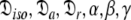
The solution to the model-free problem, as defined in Eq. 1 and when comparing the two structures, is the prolate spheroid for the 1F35 X-ray structure. The final and complete model-free results from this global diffusion model are presented in Table S5 of the supplementary material. For comparison with the original results of Gitti et al. (2005) both sets of parameter values are plotted in Fig. S2 and superimposed onto the OMP X-ray structure in both Figs. S2 and S3. Large differences in Lipari-Szabo order parameters, effective correlation times, and the Rex parameter are clearly demonstrated in the three figures.
Amplitudes of the internal motions
A number of discrepancies between the original S2 values and the reanalysis exist across the protein (Figs. S2a, 3b, and 3c). The greatest anomaly, which will be discussed below, occurs within residues 20–34 of helix α1. In addition both the N-terminus and residues 39–41 of loop 1 are more mobile in the reanalysis whereas the β-hairpin loop 4 is more restricted. Although not statistically significant on a per residue basis, systematic increases or decreases in mobility of distinct secondary structural elements has occurred. For instance all residues of helix α2 are slightly more mobile in the reanalysis. The validity of the new order parameters are strongly supported by the NMR relaxation data—many of the trends present in the R1, R2, and NOE values shown in Figure 2 of Gitti et al. (2005) are combined and reflected in the new amplitudes of motion.
Fig. 3.

Illustrations of the OMP X-ray crystallographic structure (1F35) demonstrating the differences between the results of the original model-free analysis and those of the reanalysis. The reference orientation of the structure (a) is shown as a Molmol ribbon diagram. The order parameters of (b) the original results versus (c) the new results are mapped onto the structure. For residues in which the two timescale models (m5 to m8) have been selected, the S2 values plotted are equal to  . Both the colour and bond width reflect the amplitudes of the motion. In (d) and (e) the chemical exchange parameter Rex is mapped onto the structure for the original and new analysis respectively. The greater the quantity of chemical exchange, the darker and thicker the bonds. White bonds indicate no chemical exchange whereas the bonds drawn as thin black lines represent residues for which no data was available. To accurately pinpoint the position of the motions, backbone bonds between Cα atoms are coloured rather than the bonds of the residue to which the NH vector belongs. The Molmol images were generated by macros created by relax
Rigidity of helix α1
The most striking difference between the new and the old analysis, as illustrated by Figs. S2 and 3, is the rigidity of the helix α1. In the original analysis (ibid.) helix α1 was one of the most mobile regions of the protein yet in the new analysis the helix is the most rigid secondary structure element in the protein. This rigidity is strongly supported by the original NOE values. Not only are there significant differences in the internal motions on the picosecond to nanosecond timescales (Figs. S2a, 3b, and c) but large quantities of chemical exchange which were present in the original results are absent from the reanalysis (Figs. S2c, 3d, and e). Although the R2 values of α1 are elevated above the protein average and appear to support the presence of chemical exchange the elevation is in fact caused by the geometry of the diffusion tensor. The maximum correlation time of a vector attached to a prolate tensor is when it is parallel to the long axis which, in the case of the reanalysis, is approximately 10.5 ns. The local τm values of α1 are very close to this number (Fig. 1). As was demonstrated in Table S1 and in Tjandra et al. (1996) underestimation of the global correlation time experienced by a bond vector induces artificial Rex values to appear. Notably helix α1 is parallel to the major axis of the prolate diffusion tensor (Fig. S1) hence the halving of the anisotropy will result in the underestimation of the correlation times.
The reason for the underestimation of the anisotropy of rotational diffusion in the original analysis relates to the NH bond vector distribution. A number of empirical rules were used to exclude residues from the initial tensor estimate including the low NOE rule (Kay et al. 1989; Stone et al. 1992; Barbato et al. 1992), deviations from the R2/R1 ratio (Clore et al. 1990a; Barbato et al. 1992; Tjandra et al. 1995b), and utilising solely residues within distinct secondary structure elements (Habazettl et al. 1996; Dosset et al. 2000). The consequence of implementing these commonly used exclusion rules for OMP is evident in Fig. 4—almost all residues perpendicular to the unique axis of the diffusion tensor have been removed from the analysis. Hence there is a paucity of information concerning the  eigenvalue within the limited subset of the relaxation data and extracting the true and full anisotropy of the tensor is not possible. The result is the appearance of artificial chemical exchange.
Fig. 4.

The OMP backbone amide NH bond vector orientations employed in (a, b) the original model-free analysis of Gitti et al. (2005) and (c, d) in the reanalysis using the new model-free optimisation protocol. In the original analysis the diffusion tensor was determined using residues solely within the strands of the β clam fold and helix α2 whereas in the reanalysis all residues were used. The distributions correspond surfaces draped over artificial NH vectors with the nitrogen positioned at the centre of mass of all selected residues and the bond length being set to 20 Å. Because of the symmetry of spheroidal and ellipsoidal diffusion tensors the positive or negative orientation of the XH bond has no effect on relaxation and, hence, a second artificial NH vector has been added for each residue whereby the orientation has been reversed. The PyMOL images were generated using relax
The new model-free optimisation protocol solves this issue by using all the available relaxation data for determining the diffusion tensor. No rules are used for excluding spin systems. As can be seen in Fig. 4c and d the coverage of space by the OMP amide NH bond distribution is more even and much denser. Importantly a large number of vectors sample the space parallel to the unique axis of the diffusion tensor. Hence information about all components of the diffusion tensor are adequately contained within the full set of relaxation data.
The correlation between structural quality and artificial motions
When the diffusion of the macromolecule under study is anisotropic, the accuracy of the model-free results is dependent upon the quality of the structure underlying the analysis. For a perfectly spherical probability distribution of vectors centred at the origin, the projection of the vectors onto the major axis of a spheroid will form a sinusoidal probability distribution. This distribution has zero probabilities at the poles and a maximal probability at the equator. If the orientation of an arbitrary vector attached to the molecule is slightly randomised with equal probability in all directions the mean projection of many randomisations will shift towards the equator. The projectional bias, which is purely a geometric phenomenon, has important consequences for the model-free analysis of non-spherical proteins and can have two opposing effects. If the molecule diffuses as a prolate spheroid the bias will be away from the unique, long axis causing a mean underestimation of the effective global correlation time and hence favour artificial Rex values over artificial nanosecond motions. If the molecule diffuses as an oblate spheroid the bias will be away from the unique, short axis of the tensor. The result will be a mean overestimation of the effective global correlation time and therefore artificial nanosecond motions are favoured.
The Rex values of OMP
Although loop 1, Ω-loop 3, and β-hairpin loop 4 all show significant chemical exchange in both Gitti et al. (2005) and the reanalysis, both of which chose the prolate spheroid, the scarce appearance of Rex contributions in global model MI may be an indication that the Rex values do not correspond to real chemical exchange. In the reanalysis where the X-ray crystallographic structure 1F35 was employed the residues in which Rex values appear (Fig. 3e) are all located in regions which vary significantly between the different PDB structures, as demonstrated by Figure 5 (ibid.). Because the molecule diffuses as a prolate spheroid inaccuracy in these regions of the protein will bias the model-free analysis favouring the appearance of artificial Rex values. As all Rex values in the OMP reanalysis could in fact be explained by imprecise NH backbone bond orientations either reanalysis using the RDC refined OMP structure (Wright et al. 2005) or relaxation dispersion experiments could be used to prove the presence of true chemical exchange. Alternatively the Rex contribution to the R2 relaxation rate could be eliminated prior to model-free analysis (Farrow et al. 1995; Phan et al. 1996; Kroenke et al. 1999; Butterwick et al. 2004).
Failure of the diffusion seeded paradigm
The reason for the artificial Rex values of helix α1 was identified as a failure of the diffusion seeded model-free paradigm rather than an optimisation, model selection, or model failure issue. By taking the diffusion parameters of the prolate core of the hybrid model (vide supra) as a starting point for model-free analysis, the diffusion seeded protocol was employed within relax. The prolate spheroid was chosen by AIC model selection. Convergence of this model occurred after six iterations and the final geometric parameters were  = {τm: 9.00 ns;
  : 4.5e7 s−1}. Sliding between universes to reach the universal solution
  did not occur and the artificial motions of the protein were still present. Finding the solution was only possible using either the new model-free optimisation protocol or that of Orekhov et al. (1999a).
The internal correlation times
Another major difference between the original results and the reanalysis, as demonstrated in Figs. S2b and S3, is the internal model-free correlation times. Originally only 42 correlation times were extracted whereas in the reanalysis 102 correlation times were selected, the additional correlation times spanning from 10 ps to well into the nanosecond range. The differences are primarily due to the more parsimonious AIC model selection. In the original analysis the ANOVA step-up hypothesis testing model selection which is coded into the FAST-modelfree interface (Cole and Loria 2003) to the Modelfree program (Palmer et al. 1991; Mandel et al. 1995) and based on the step-up methodology of Mandel et al. (1995) was employed. A significant patch of nanosecond motions occurs on the β-hairpin loop 4 side of the β clam fold. However as these motions are not present in global model MI (data not shown) and the loop positions are quite variable between the X-ray and two NMR structures (Baldisseri et al. 2002; Smith et al. 2002; Wright et al. 2005), these slow nanosecond motions may be artificial (Schurr et al. 1994).
Parameter uncertainties
In Fig. S2 it is evident that the parameter errors in the reanalysis are greater than those of the original results. This is due to two factors: the effects of under-fitting and the higher precision optimisation coupled with Monte Carlo simulations. As more parameters are utilised in the reanalysis, greater amounts of noise from the collected relaxation data are transferred into the model (d’Auvergne and Gooley 2003). The deliberate under-fitting of the ANOVA step-up model selection (Mandel et al. 1995) of the original analysis not only skews the dynamic picture but also results in an underestimation of the parameter uncertainties. Higher precision optimisation also results in greater, yet real, parameter uncertainties. The model-free parameter errors are determined via Monte Carlo simulation whereby each simulation is minimised using the same optimisation algorithms as the original data. The initial position for MC simulations is set to the optimised model-free parameter values hence if optimisation terminates early due to low precision or other issues (Paper I) then the affected simulation does not move as far away from the mean as it should. The result is that the parameter errors are underestimated.
Conclusion
The diffusion seeded model-free paradigm of using an initial estimate of the diffusion tensor has been used in most model-free analyses presented in the literature. There are, however, a number of problems associated with the approach (d’Auvergne and Gooley 2007b). To avoid these this paper presents a new model-free optimisation protocol which completely reverses the logic of the diffusion seeded model-free paradigm. Rather than starting with the diffusion tensor the protocol begins by optimising the model-free models free of any global diffusion parameters. This is done by constructing the global model MI in which each bond vector has a local τm parameter. Model-free models tm0 to tm9 are optimised and the best model selected. In the next step of the protocol the local τm parameter is removed from the models, the model-free parameters are held fixed, and the spherical diffusion tensor (global model MII), prolate spheroid (MIII), oblate spheroid (MIV), and ellipsoid (MV) parameters are optimised. Iterative steps of optimisation of models m0 to m9 with the diffusion parameters fixed, model elimination, AIC model selection, and then optimisation of all spin systems are performed until convergence. This protocol is designed for robustly finding the universal solution  defined in Eq. 1. By using the synthetic data from Schurr et al. (1994) and the bacteriorhodopsin fragment (1-36)BR data (Orekhov et al. 1999a) the new protocol is shown to avoid all of the problems associated with model-free analysis. These include artificial nanosecond motions (Schurr et al. 1994), artificial chemical exchange (Tjandra et al. 1996), two minima of spheroidal parameter space (Paper I), and violation of the rigidity assumption and hiding of nanosecond motions.
In using AIC model selection to choose between the model-free models as well as the diffusion tensors (d’Auvergne and Gooley 2003); implementing model elimination to remove failed models (d’Auvergne and Gooley 2006); employing Newton optimisation together with the backtracking line search (Nocedal and Wright 1999) and Gill, Murray, Wright Hessian modification (Gill et al. 1981) and constraining the parameters with the Augmented Lagrangian algorithm (Nocedal and Wright 1999; d’Auvergne and Gooley 2007a); minimising the numerically stabilised model-free equations (d’Auvergne and Gooley 2007a); and utilising the new model-free optimisation protocol to find the universal solution  a significantly improved and refined picture of the dynamics of a macromolecule can be obtained.
Electronic supplementary material
Below is the link to the electronic supplementary material.
Acknowledgements
We would like to thank Vladislav Orekhov and Dmitry Korzhnev for kindly donating the relaxation data of the bacteriorhodopsin (1-36)BR fragment.
Abbreviations
- AIC
Akaike’s Information Criteria
- ANOVA
Analysis of variance
- BIC
Schwarz or Bayesian Information Criteria
- CSA
Chemical Shift Anisotropy
- ΔK–L
Kullback–Leibler discrepancy

Set of diffusion tensor parameters

Set of model-free parameters for a single spin system

Set of geometric diffusion parameters
- GMW
Gill, Murray, and Wright Hessian modification

Set of all global models

- MC
Monte Carlo

Set of orientational diffusion parameters
- OMP
Olfactory Marker Protein

The global model, space, or universe

Set of model-free parameters and local τm for a single spin system

Universal set

Universal solution
- XH bond
Heteronucleus-proton bond
Footnotes
Electronic supplementary material
The online version of this article (doi:10.1007/s10858-007-9213-3) contains supplementary material, which is available to authorized users.
References
- Akaike H (1973) Information theory and an extension of the maximum likelihood principle. In: Petrov BN, Csaki F (eds) Proceedings of the second international symposium on information theory. Budapest, Akademia Kiado, pp 267–281
- Baldisseri DM, Margolis JW, Weber DJ, Koo JH, Margolis FL (2002) Olfactory marker protein (OMP) exhibits a beta-clam fold in solution: implications for target peptide interaction and olfactory signal transduction. J Mol Biol 319(3):823–837 [DOI] [PubMed]
- Barbato G, Ikura M, Kay LE, Pastor RW, Bax A (1992) Backbone dynamics of calmodulin studied by 15N relaxation using inverse detected two-dimensional NMR spectroscopy: the central helix is flexible. Biochemistry 31(23):5269–5278 [DOI] [PubMed]
- Brüschweiler R, Liao X, Wright PE (1995) Long-range motional restrictions in a multidomain zinc-finger protein from anisotropic tumbling. Science 268(5212):886–889 [DOI] [PubMed]
- Burnham KP, Anderson DR (1998) Model selection and inference: a practical information-theoretic approach. Springer-Verlag, New York
- Butterwick JA, Loria PJ, Astrof NS, Kroenke CD, Cole R, Rance M, Palmer AG 3rd (2004) Multiple time scale backbone dynamics of homologous thermophilic and mesophilic ribonuclease HI enzymes. J Mol Biol 339(4):855–871 [DOI] [PubMed]
- Chen J, Brooks CL, 3rd, Wright PE (2004) Model-free analysis of protein dynamics: assessment of accuracy and model selection protocols based on molecular dynamics simulation. J Biomol NMR 29(3):243–257 [DOI] [PubMed]
- Clore GM, Driscoll PC, Wingfield PT, Gronenborn AM (1990a) Analysis of the backbone dynamics of interleukin-1 beta using two-dimensional inverse detected heteronuclear 15N-1H NMR spectroscopy. Biochemistry 29(32):7387–7401 [DOI] [PubMed]
- Clore GM, Szabo A, Bax A, Kay LE, Driscoll PC, Gronenborn AM (1990b) Deviations from the simple 2-parameter model-free approach to the interpretation of N-15 nuclear magnetic-relaxation of proteins. J Am Chem Soc 112(12):4989–4991 [DOI]
- Cole R, Loria J (2003) FAST-Modelfree: a program for rapid automated analysis of solution NMR spin-relaxation data. J Biomol NMR 26(3):203–213 [DOI] [PubMed]
- d’Auvergne EJ (2006) Protein dynamics: a study of the model-free analysis of NMR relaxation data. Ph.D. thesis, Biochemistry and Molecular Biology, University of Melbourne. http://eprints.infodiv.unimelb.edu.au/archive/00002799/
- d’Auvergne EJ, Gooley PR (2003) The use of model selection in the model-free analysis of protein dynamics. J Biomol NMR 25(1):25–39 [DOI] [PubMed]
- d’Auvergne EJ, Gooley PR (2006) Model-free model elimination: a new step in the model-free dynamic analysis of NMR relaxation data. J Biomol NMR 35(2):117–135 [DOI] [PubMed]
- d’Auvergne EJ, Gooley PR (2007a) Optimisation of NMR dynamic models I. Minimisation algorithms and their performance within the model-free and Brownian rotational diffusion spaces. J Biomol NMR. doi:10.1007/s10858-007-9214-2 [DOI] [PMC free article] [PubMed]
- d’Auvergne EJ, Gooley PR (2007b) Set theory formulation of the model-free problem and the diffusion seeded model-free paradigm. Mol BioSyst 3(7):483–494 [DOI] [PubMed]
- DeLano WL (2002) The PyMOL molecular graphics system. http://www.pymol.org
- Dosset P, Hus JC, Blackledge M, Marion D (2000) Efficient analysis of macromolecular rotational diffusion from heteronuclear relaxation data. J Biomol NMR 16(1):23–28 [DOI] [PubMed]
- Farrow NA, Zhang OW, Szabo A, Torchia DA, Kay LE (1995) Spectral density-function mapping using N-15 relaxation data exclusively. J Biomol NMR 6(2):153–162 [DOI] [PubMed]
- Gagné SM, Tsuda S, Spyracopoulos L, Kay LE, Sykes BD (1998) Backbone and methyl dynamics of the regulatory domain of troponin C: anisotropic rotational diffusion and contribution of conformational entropy to calcium affinity. J Mol Biol 278(3):667–686 [DOI] [PubMed]
- Gill PE, Murray W, Wright MH (1981) Practical optimization. Academic Press
- Gitti RK, Wright NT, Margolis JW, Varney KM, Weber DJ, Margolis FL (2005) Backbone dynamics of the olfactory marker protein as studied by 15N NMR relaxation measurements. Biochemistry 44(28):9673–9679 [DOI] [PubMed]
- Habazettl J, Myers LC, Yuan F, Verdine GL, Wagner G (1996) Backbone dynamics, amide hydrogen exchange, and resonance assignments of the DNA methylphosphotriester repair domain of Escherichia coli Ada using NMR. Biochemistry 35(29):9335–9348 [DOI] [PubMed]
- Horne J, d’Auvergne EJ, Coles M, Velkov T, Chin Y, Charman WN, Prankerd R, Gooley PR, Scanlon MJ (2007) Probing the flexibility of the DsbA oxidoreductase from Vibrio cholerae—a 15N–1H heteronuclear NMR relaxation analysis of oxidized and reduced forms of DsbA. J Mol Biol 371(3):703–716 [DOI] [PubMed]
- Kay LE, Torchia DA, Bax A (1989) Backbone dynamics of proteins as studied by 15N inverse detected heteronuclear NMR spectroscopy: application to staphylococcal nuclease. Biochemistry 28(23):8972–8979 [DOI] [PubMed]
- Korzhnev DM, Billeter M, Arseniev AS, Orekhov VY (2001) NMR studies of Brownian tumbling and internal motions in proteins. Prog NMR Spectrosc 38(3):197–266 [DOI]
- Korzhnev DM, Orekhov VY, Arseniev AS (1997) Model-free approach beyond the borders of its applicability. J Magn Reson 127(2):184–191 [DOI] [PubMed]
- Kroenke CD, Rance M, Palmer AG (1999) Variability of the N-15 chemical shift anisotropy in Escherichia coli ribonuclease H in solution. J Am Chem Soc 121(43):10119–10125 [DOI]
- Kullback S, Leibler RA (1951) On information and sufficiency. Ann Math Stat 22(1):79–86 [DOI]
- Lee LK, Rance M, Chazin WJ, Palmer AG (1997) Rotational diffusion anisotropy of proteins from simultaneous analysis of N-15 and C-13(alpha) nuclear spin relaxation. J Biomol NMR 9(3):287–298 [DOI] [PubMed]
- Linhart H, Zucchini W (1986) Model selection, Wiley Series in Probability and mathematical statistics. John Wiley & Sons, Inc New York
- Lipari G, Szabo A (1982a) Model-free approach to the interpretation of nuclear magnetic-resonance relaxation in macromolecules I. Theory and range of validity. J Am Chem Soc 104(17):4546–4559 [DOI]
- Lipari G, Szabo A (1982b) Model-free approach to the interpretation of nuclear magnetic-resonance relaxation in macromolecules II. Analysis of experimental results. J Am Chem Soc 104(17):4559–4570 [DOI]
- Luginbühl P, Pervushin KV, Iwai H, Wüthrich K (1997) Anisotropic molecular rotational diffusion in 15N spin relaxation studies of protein mobility. Biochemistry 36(24):7305–7312 [DOI] [PubMed]
- Mandel AM, Akke M, Palmer AG, 3rd (1995) Backbone dynamics of Escherichia coli ribonuclease HI: correlations with structure and function in an active enzyme. J Mol Biol 246(1):144–163 [DOI] [PubMed]
- Mandel AM, Akke M, Palmer AG, 3rd (1996) Dynamics of ribonuclease H: temperature dependence of motions on multiple time scales. Biochemistry 35(50):16009–16023 [DOI] [PubMed]
- Nocedal J, Wright SJ (1999) Numerical optimization, Springer Series in Operations research. Springer-Verlag, New York
- Orekhov VY, Korzhnev DM, Diercks T, Kessler H, Arseniev AS (1999a) H-1-N-15 NMR dynamic study of an isolated alpha-helical peptide (1-36)- bacteriorhodopsin reveals the equilibrium helix-coil transitions. J Biomol NMR 14(4):345–356 [DOI]
- Orekhov VY, Korzhnev DM, Pervushin KV, Hoffmann E, Arseniev AS (1999b) Sampling of protein dynamics in nanosecond time scale by 15N NMR relaxation and self-diffusion measurements. J Biomol Struct Dyn 17(1):157–174 [DOI] [PubMed]
- Orekhov VY, Pervushin KV, Korzhnev DM, Arseniev AS (1995) Backbone dynamics of (1-71)Bacterioopsin and (1-36)Bacterioopsin studied by 2-dimensional H-1-N-15 NMR-spectroscopy. J Biomol NMR 6(2):113–122 [DOI] [PubMed]
- Palmer AG, Rance M, Wright PE (1991) Intramolecular motions of a zinc finger DNA-binding domain from Xfin characterized by proton-detected natural abundance C-12 heteronuclear NMR-spectroscopy. J Am Chem Soc 113(12):4371–4380 [DOI]
- Phan IQH, Boyd J, Campbell ID (1996) Dynamic studies of a fibronectin type I module pair at three frequencies: anisotropic modelling and direct determination of conformational exchange. J Biomol NMR 8(4):369–378 [DOI] [PubMed]
- Schurr JM, Babcock HP, Fujimoto BS (1994) A test of the model-free formulas. Effects of anisotropic rotational diffusion and dimerization. J Magn Reson B 105(3):211–224 [DOI] [PubMed]
- Schwarz G (1978) Estimating dimension of a model. Ann Stat 6(2):461–464 [DOI]
- Smith PC, Firestein S, Hunt JF (2002) The crystal structure of the olfactory marker protein at 2.3 A resolution. J Mol Biol 319(3):807–821 [DOI] [PubMed]
- Stone MJ, Fairbrother WJ, Palmer AG, Reizer J, Saier MH, Wright PE (1992) Backbone dynamics of the Bacillus subtilis glucose permease-IIA domain determined from N-15 NMR relaxation measurements. Biochemistry 31(18):4394–4406 [DOI] [PubMed]
- Tjandra N, Feller SE, Pastor RW, Bax A (1995a) Rotational diffusion anisotropy of human ubiquitin from N-15 NMR relaxation. J Am Chem Soc 117(50):12562–12566 [DOI]
- Tjandra N, Kuboniwa H, Ren H, Bax A (1995b) Rotational dynamics of calcium-free calmodulin studied by 15N-NMR relaxation measurements. Eur J Biochem 230(3):1014–1024 [DOI] [PubMed]
- Tjandra N, Wingfield P, Stahl S, Bax A (1996) Anisotropic rotational diffusion of perdeuterated HIV protease from 15 N NMR relaxation measurements at two magnetic fields. J Biomol NMR 8(3):273–284 [DOI] [PubMed]
- Woessner DE (1962) Nuclear spin relaxation in ellipsoids undergoing rotational brownian motion. J Chem Phys 37(3):647–654 [DOI]
- Wright NT, Margolis JW, Margolis FL, Weber DJ (2005) Refinement of the solution structure of rat olfactory marker protein (OMP). J Biomol NMR 33(1):63–68 [DOI] [PubMed]
- Zucchini W (2000) An introduction to model selection. J Math Psychol 44(1):41–61 [DOI] [PubMed]
Associated Data
This section collects any data citations, data availability statements, or supplementary materials included in this article.
Supplementary Materials
Below is the link to the electronic supplementary material.