

SUMMARY
The problem of analyzing a continuous variable with a discrete component is addressed within the frame-work of the mixture model proposed by Moulton and Halsey. The model can be generalized by the introduction of the log-skew-normal distribution for the continuous component, and the fit can be significantly improved by its use, while retaining the interpretation of regression parameter estimates. Simulation studies and application to a real data set are used for demonstration.
Keywords: censoring, skew-normal distribution, two-part model
1. INTRODUCTION
Investigators are often confronted with data in which the recorded continuous outcome variable has a lower bound (considered here to be at zero) and takes on this boundary value for a sizeable fraction of sample observations. The concentration of observations at zero could arise from several circumstances.
The observed values are ‘true’ zeros. An example of this is provided by household expenditures on a particular type of durable good over a certain period of time, in which many households do not purchase the good, and thus their actual expenditure is zero.
The measurements are subject to detection limits, and most or all zero observations would be positive if the measurement process were more sensitive. This is a common phenomenon in clinical laboratory studies of quantitative assays of circulating biochemicals.
Still another possible scenario is a measurement which is zero for technical reasons, e.g. due to environmental or physical factors, that do not imply that the true value, if it had been properly observed, would have been a ‘low value’. One might well wish to consider these observations as missing. However, the researcher may not even be aware of such a technical problem, either in general or in any specific observation, and therefore may be unable to classify these observations into those that should be regarded as ‘missing’ versus those that should be considered ‘low.’
It is well known that conventional regression analysis may not be an adequate method for making inferences in the presence of such a point mass at the low end of the measurement scale. One can resort to binary-response analysis techniques (e.g. probit or logistic analysis) if one is willing to restrict attention to the probabilities of limit and non-limit responses. Given such a framework, these binary response models represent adequate statistical models. However, they are inefficient if the goal is to extract all the information both in the limiting response and in the continuous response. Although more details can be retained if one arbitrarily forms an ordinal response out of the continuous data, only analysis that combines the continuous information with the binary data can be fully efficient.
Another approach to dealing with the zeros is to treat them as latent (unobserved) continuous observations that have been left-censored. This idea was popularized by Tobin [1] and the resulting model is commonly referred to as the Tobit model. Mathematically, the Tobit model can be formulated as
where the latent variable . Here and henceforth we denote the observed outcome by yi,i =1,...,n, the values of k explanatory variables for the ith observation by , the regression parameters by β = (β0 ,..., βk)T and the ith residual term by εi. Although the interpretation of the negative latent observations can be slightly ambiguous, the Tobit specification is usually appropriate for the situation in which the sample proportion of zeros is roughly equivalent to the left tail area of the assumed parametric distribution. Such a specification has interpretational difficulties, however, when there is an excess of limit responses above what would be implied by the tail area of the relevant parametric distribution.
The model proposed by Cragg [2], often called the two-part model, provides us with a way to relax the tail-probability constraint of the Tobit specification. In essence, a two-part model is a binary mixture model formed from a linear combination of a positive continuous distribution (possibly left truncated) and a point distribution located at zero. More formally, the probability density function of an outcome yi under Cragg’s specification can be expressed in the following form
| (1) |
where Ii is an indicator function taking value one if yi =0 and zero otherwise, pi is the probability determining the relative contribution made by the point distribution to the overall mixture distribution, and f+ is a density function with positive support. In this model, the occurrence of limit responses and the size of the non-limit responses are determined by separate stochastic processes, allowing additional observations at the low end and two possibly distinct sets of covariates to be related to pi and f+, respectively. Note that any positive observation necessarily comes from f+ while a recorded zero is generated from the point distribution. This clearly restricts other reasonable determinants of zero observations but may be sensible in terms of the way the data are obtained.
Moulton and Halsey [3] generalized the two-part model by explicitly allowing for the possibility that some limit responses are the result of interval censoring from f+. This means that an observed zero can be either a realization from the point distribution or a partial observation from f+ with actual value not precisely known but lying somewhere in (0, T) for a small pre-specified constant T. Formally,
| (2) |
where F+ is the corresponding probability function of f+. Irrespective of whether or not censoring is present, a useful family of distributional specifications can be imposed upon the outcome variable by varying the choices for the basis distribution f+ and the link function of the mixing probability pi. Specifications that have been studied include (1) a hybrid of probit modeling for pi and a truncated normal density for f+ [2], (2) a composite between a logit link and a lognormal distribution [3], and (3) a logit/log-gamma coupling [4]. Although these combinations may often be adequate, the reliability of the analytic results in any given situation depends on the capability of the assumed density to model the characteristics of the specific data under study.
Considerations such as computational simplicity and the central limit theorem have traditionally suggested the normal or lognormal distributions as obvious candidates for f+ in model (1). However, inasmuch as f+ and pi in model (2) are intimately linked, we would anticipate that the assumed shape of f+ to have a profound impact on statistical inferences from this model. A well-recognized limitation of the normal distribution is its inability to account for asymmetry, a common feature of many sets of data, notably those restricted to the positive axis. In the setting of right skewness, a customary statistical approach is to apply a logarithmic transformation. However, this method is ad hoc and may or may not optimally account for the distributional features of the data. It is preferable to introduce less restrictive families of distributions that can accommodate asymmetry in a more flexible way in order to properly model the data. It is the intention of this communication to examine the suitability of the skew normal distribution (see Genton [5] for a review) in fitting the logarithm of the positive responses, as a means of allowing but not restricting the fit to a normal distribution. More specifically, our focus is to propose a probit/log-skew-normal model for data analysis using the likelihood approach.
The remainder of this paper is structured as follows. After a concise review of the definition and some key properties of the skew-normal distribution in Section 2, Section 3 derives the probit/log-skew-normal model that incorporates two sets of covariates. In Section 4, we motivate and demonstrate the potential of the proposed model through an actual data set involving the coronary artery calcification (CAC) scores from an atherogenesis study. The outputs are contrasted with those acquired under the probit/lognormal model. A probit/log-gamma regression simulation example aiming to show the aptness of the log-skew-normal representation to account for skewness in the continuous component is presented in Section 5. Finally, the paper concludes with a few summary remarks in Section 6.
2. THE SKEW-NORMAL DISTRIBUTION
The term skew normal refers to a rich class of continuous distribution that contains the normal density as a proper member. In the univariate setting, the family has received attention in the literature under a few different versions, see, for example, Azzalini [6, 7], John [8], and Mudholkar and Hutson [9]. One such class of distributions was proposed by Branco and Dey [10], and later extended by Sahu et al. [11]. These authors introduced asymmetry into any symmetric distribution via simple transformation and conditioning techniques. As a special case, a random variable Z is said to have a skew normal distribution with skewness parameter δ if its probability density function is
where ϕ(·) and Φ(·) denote the standard normal density and cumulative distribution functions, respectively. We write Z ~SN(μ,σ,δ) for future reference. The corresponding unimodal density is positively skewed when δ is larger than zero, skewed to the left when δ takes a negative value, and reduces to a normal density when δ=0. Since distributional skewness is regulated by
| (3) |
δ,it is reasonable to regard δ as the skewness parameter. The mean and variance of Z are given, respectively, by Heuristically, instead of considering the commonly used ad hoc transformation for symmetry in normal theory statistics, the skew normal distribution offers us an appealing alternative to deal with asymmetry in empirical data. In particular, it allows us to perform model fitting on the original scale of the data and hence leads to more meaningful interpretation of the quantities involved.
3. THE PROBIT/LOG-SKEW-NORMAL MODEL WITH INTERVAL CENSORING
The mixture model we consider is given by equation (2) in the Introduction. Note that two things are needed to complete the specification of the model: a link function for pi and a density function for f+. The specific stochastic model studied here is
in which the observed data yi are independently, identically distributed random variables. In effect, the set of explanatory variables x(1) = (x(1)1,..., x(1)n)T governs the probability of a true zero response, whereas the magnitude of the censored non-limit response is determined by x(2) = (x(2)1,..., x(2)n)T. As a consequence of allowing for possibly different sets of covariates to be associated with pi and f+, the model has the potential of leading to more accurate and informative regression analysis. Note that the reason for modeling the positive outcome on the logarithmic scale, log(yi|yi >0), instead of on the original scale, yi|yi >0, is to ensure a positive estimation on the limited response variable.
Let h(·) and H(·) be the skew normal density function and distribution function, respectively. The likelihood contribution from the logarithm of the ith observation is easily expressed namely
Owing to the independence assumption, the likelihood function to be maximized is just the product of li,i =1,...,n. This likelihood is rather complicated to allow exploration by analytical means; hence numerical methods are employed instead. We evaluate H(·) by using the Laguerre quadrature and resort to the double dogleg algorithm for maximum likelihood estimation. The double dogleg algorithm couples the quasi-Newton and trust region methods and works well for medium-to-large problems (see Dean [12] and references therein for further details).
4. CAC SCORES EXAMPLE
Atherosclerotic coronary artery disease is a major cause of mortality and morbidity in industrialized nations. CAC, a widely used surrogate for coronary atherosclerotic burden, can be detected noninvasively by electron beam computed tomography. The amount of calcium is usually assessed through the use of the Agatston scoring method [13]. The resulting CAC scores can range from zero to several thousands. Such a measure facilitates an investigation of the relationship between subclinical coronary artery atherosclerosis and its risk factors in asymptomatic adults. Our example is based on data from the subjects in the ongoing Functional Arterial Changes in Atherogenesis Study [14] being conducted in Rochester, Minnesota. The study group was recruited from the community-based Epidemiology of Coronary Artery Calcification (ECAC) Study (see Kaufmann et al. [15] for some background information) during September 2002-November 2004. It refers to a sample of 471 non-Hispanic white participants who had no previous report of myocardial infarction, stroke, coronary angioplasty or coronary bypass, or cardiac transplant surgery. The data analyzed in the current example were collected on these individuals as part of the ECAC study itself.
For the purposes of this illustration, we are interested in characterizing the dependence of CAC score on conventional risk factors for coronary atherosclerosis. Thus, we regard the response variable to be CAC score, and we take age, sex, body mass index (BMI), hypertension, smoking history, diabetes, total cholesterol, HDL cholesterol, and statin use as our explanatory variables. There are three subjects with missing measurements. We assume that the data are missing at random and omit them from the present study. A histogram depicting the distribution of CAC score is presented in Figure 1. Among the 468 individuals with complete data, 177 (37.8 per cent) had a recorded CAC score of zero. Because of the highly skewed nature of the distribution of CAC score, a better graphical representation would be provided by the histogram of log (CAC+1). The histogram is also shown in Figure 1, which clearly suggests a mixture of a point distribution at zero and a continuous distribution on the positive side. Consequently, modeling using a Tobit model is likely to lead to biased inferences since there are far more left-censored observations than would be expected under the Tobit formulation. The two-part models offer us a viable framework to deal adequately with the excess of zeros.
Figure 1.

Histograms of the coronary artery calcification (CAC) scores with observed values shown as symbols on the horizontal axis. The bin in gray corresponds to the zero CAC scores.
The probit/log-skew-normal model developed in Section 3 is used for the analysis of the CAC data. Our primary aims here are (a) to examine the skew normal distribution in fitting the logarithm of the positive CAC score from the viewpoint of reliable analysis and (b) to contrast the results obtained under the proposed models with those from the probit/lognormal models. Hence, a total of four sampling models are fitted to the data. Briefly they are probit/lognormal without censoring, probit/lognormal with censoring, probit/log-skew-normal without censoring, and probit/log-skew-normal with censoring. For the models with censoring, we regard T = 1.0 as the detection limit of CAC score, i.e. some recorded zeros belong to the left tail of the upper distribution. Observe in Figure 1 that there are 13 observations with the smallest positive CAC score of 1.38, causing an appreciable bump on the lower end of the distribution of log (CAC+1). This has to do with the discrete nature of the image processing software at the extreme of the distribution. These are also treated as having been left-censored, but at 1.38, in the two censoring models.
An explanatory variable in a two-part model may be related either to the probability of obtaining a null response (CAC score=0) or to the magnitude of a positive CAC score, or to both. Starting from all covariates in both components of the probit/lognormal models, we determine significant predictors of the outcome variable by performing backward elimination with p-value <0.05 retention level. The resulting final sets of covariates are then fixed and applied to probit/log-skew-normal models so as to study the effect of asymmetry. Table I reports the maximum likelihood parameter estimates based on double dogleg algorithm for the final models. For the sake of completeness, the results from probit and Tobit analyses are also included in the same table.
Table I.
Parameter estimates and the associated standard errors (given in parentheses) for the coronary artery calcification scores example
| Model | β0 | βage | βmale | βBMI | βhyperten | βsmoke | βstatin | σ | δ |
|---|---|---|---|---|---|---|---|---|---|
| Probit [Y =0/1] | 5.123 (0.632) |
-0.062 (0.008) |
-0.921 (0.138) |
-0.041 (0.013) |
— |
— |
-0.544 (0.168) |
— |
— |
| Tobit [Y = log(CAC+1)] | -13.002 (1.453) |
0.175 (0.017) |
2.450 (0.295) |
0.069 (0.029) |
0.8173 (0.340) |
0.743 (0.287) |
1.573 (0.335) |
2.845 (0.128) |
— |
| Probit/lognormal without censoring | 5.123 (0.631) -2.403 (0.745) |
-0.062 (0.007) 0.083 (0.011) |
-0.921 (0.138) 0.974 (0.201) |
-0.041 (0.013) — |
— 0.605 (0.219) |
— 0.624 (0.195) |
-0.544 (0.169) 0.848 (0.215) |
— 1.634 (0.068) |
— — |
| Probit/log-skew-normal without censoring | 5.123 (0.631) -0.513 (0.716) |
-0.062 (0.008) 0.084 (0.010) |
-0.921 (0.138) 1.002 (0.187) |
-0.041 (0.013) — |
— 0.462 (0.198) |
— 0.525 (0.180) |
-0.544 (0.168) 0.912 (0.197) |
— 0.897 (0.146) |
— -2.302 (0.230) |
| Probit/lognormal with censoring | 4.789 (0.687) -3.704 (0.932) |
-0.058 (0.008) 0.098 (0.014) |
-0.887 (0.148) 1.130 (0.241) |
-0.041 (0.014) — |
— 0.680 (0.256) |
— 0.737 (0.229) |
-0.508 (0.177) 0.915 (0.249) |
— 1.820 (0.095) |
— — |
| Probit/log-skew-normal with censoring | 5.087 (0.857) -1.500 (0.830) |
-0.060 (0.010) 0.106 (0.013) |
-0.978 (0.193) 1.106 (0.215) |
-0.052 (0.019) — |
— 0.414 (0.211) |
— 0.583 (0.195) |
-0.570 (0.247) 1.021 (0.216) |
— 0.604 (0.148) |
— -3.873 (0.482) |
Diabetes, total cholesterol, and HDL cholesterol were discarded during the process of backward elimination.
Age, sex, and statin use are important predictors in both components of the two-part models. BMI figures strongly only in the probit component. In contrast, hypertension and smoking history play a vital role only in the continuous distribution component. The effect of hypertension is fairly significant in the probit/lognormal models (p-value=0.006 without censoring, p-value=0.008 with censoring), but it is attenuated by assuming asymmetry (p-value=0.02 without censoring, p-value=0.05 with censoring). If backward elimination method were to be employed, hypertension would not have stayed in the censored probit/log-skew-normal model. The coefficients in the probit component of the two-part models with no censoring are essentially identical, as expected, to those acquired under the probit model. Interestingly, when censoring is assumed, the absolute values of these estimates in the symmetric model are notably larger than those in the skewed model. Inspection of the estimated values in the continuous distribution component indicates relatively little alteration in the inferences on βage, βmale, βBMI,and βstatin but more alteration in those on β0, βhyperten, βsmoke,and σ after allowing for skewness. The notably different estimates of β0 and σ are easily justifiable since the parameters have dissimilar interpretations. In the skewed models, from equation (3), β0 does not represent the regression intercept, and δ shares the data variability with σ. These distinctions from the probit/lognormal models render the corresponding estimates non-comparable.
The p-values of δ in the models with or without censoring are both <0.001, implying that a skewed model is needed to fit the logarithmic transform of the continuous component of the data. This hypothesis can also be tested by likelihood-ratio method as the log-skewed model contains the lognormal model as a special case. The test statistic is 10.8 for non-censoring models and is 25.7 for censoring models. Thus, when compared with a χ2(1) critical value, the tests provide overwhelmingly strong evidence against the null hypothesis that δ=0.
In an attempt to check the quality of model fits, Figure 2 plots the fitted densities under the Tobit and each of the two-part models, together with a histogram of the logarithm of the positive CAC scores. The inappropriateness of the Tobit fit is readily seen from the diagram, lending support to our earlier claim that the Tobit model would lead to misleading results when there are an excess of zeros in the response. All two-part models seem to provide a satisfactory overall representation to the underlying data. However, the probit/lognormal models need to induce a leftward shift, especially when censoring is assumed, so as to account for the skewness in the data. The fitted density of the probit/log-skew-normal with censoring model possesses a far heavier left-tail than its symmetric counterpart. Recall that the observed zero CAC scores are shared between the point and continuous distributions in the censoring models. Thus, there are substantially more zeros belonging to the left-tail of the continuous distribution in the probit/log-skew-normal model (21 per cent) than in the probit/lognormal model (6 per cent). The estimated proportions of observations coming from the point distribution are 37.6 per cent (without censoring) and 35.3 per cent (with censoring) under the symmetric models, and 37.6 per cent (without censoring) and 25.8 per cent (with censoring) under the skewed models. If the data-generating mechanisms were to be followed, there would be 37.6 per cent estimated recorded zeros in both censoring models, close to the sample proportion of 37.8 per cent. It is worth noting that the Tobit model underestimates the proportion of recorded zeros by 6.1 per cent.
Figure 2.

Histograms of the logarithm of the positive coronary artery calcification (CAC) scores with superimposed fitted densities from various models. The observed values are shown as symbols on the horizontal axis. The shaded bin corresponds to left-censored observations.
5. SIMULATION STUDIES
It is of interest to assess the ability of the log-skew-normal density in reflecting varying degrees of asymmetry in the distribution of the non-limit responses when the underlying distribution comes from a different family. To this end, three simulation studies were conducted based on the two-part model as follows:
| (4) |
where εi follows a standard log-gamma distribution [4, 16] with probability density
Here Γ(·) denotes the gamma function. The main motivation for considering the log-gamma distribution was that, similar to the skew normal distribution, it utilizes a single parameter to index a wide range of degrees of skewness. Note that no partial observation was assumed in the studies for the purposes of exposition.
We generated 500 independent standard normal observations for the explanatory variable x and assigned α0 =1 ,β0 =-0.5, α1 =-2, β1 =1, and σ=1. The parametric value of q was specified as 0, 0.5, and 2, yielding error distributions (on the log scale) with no skewness, moderate skewness, and high skewness, respectively. Using the same set of xi samples, 1000 data sets were simulated from model (4) for each of the three values of q.
We fit each simulated data set to a probit/log-skew-normal model. The true probit/log-loggamma model was also fit for comparison. Table II records the summary values of the numerical work. Scrutinizing the table reveals remarkably consistent findings in the probit component over the two models. This is not surprising given that the probit and continuous distribution components are completely separable in the likelihood.
Table II.
Monte Carlo results for the simulated example
| Probit/log-skew-normal |
Probit/log-log-gamma |
||||||
|---|---|---|---|---|---|---|---|
| Parameter | MC result | Scenario 1 | Scenario 2 | Scenario 3 | Scenario 1 | Scenario 2 | Scenario 3 |
| α0 (1) | MC mean | 0.909 | 1.010 | 1.008 | 0.909 | 1.010 | 1.008 |
| MC SD | 0.070 | 0.074 | 0.077 | 0.070 | 0.074 | 0.077 | |
| Average SE | 0.069 | 0.074 | 0.074 | 0.069 | 0.074 | 0.074 | |
| β0(-0.5) | MC mean | -0.427 | -0.504 | -0.506 | -0.427 | -0.504 | -0.506 |
| MC SD | 0.070 | 0.075 | 0.075 | 0.070 | 0.075 | 0.075 | |
| Average SE | 0.068 | 0.073 | 0.073 | 0.068 | 0.073 | 0.073 | |
| α1 | MC mean | -1.097 | -1.163 | -1.977 | -2.065 | -2.001 | -1.995 |
| MC SD | 0.069 | 0.115 | 0.589 | 0.121 | 0.080 | 0.079 | |
| Average SE | 0.068 | 0.112 | 0.456 | 0.114 | 0.080 | 0.079 | |
| β1 (1) | MC mean | 0.989 | 1.001 | 0.999 | 0.994 | 1.000 | 0.999 |
| MC SD | 0.052 | 0.051 | 0.050 | 0.051 | 0.050 | 0.050 | |
| Average SE | 0.051 | 0.050 | 0.050 | 0.051 | 0.050 | 0.050 | |
| σ | MC mean | 0.276 | 0.651 | 0.893 | 0.995 | 0.991 | 0.994 |
| MC SD | 0.059 | 0.078 | 0.069 | 0.076 | 0.040 | 0.036 | |
| Average SE | 0.059 | 0.076 | 0.123 | 0.073 | 0.039 | 0.035 | |
| δ or q | MC mean | -2.783 | -1.372 | -0.023 | 1.785 | 0.496 | 0.002 |
| MC SD | 0.120 | 0.139 | 0.733 | 0.216 | 0.123 | 0.121 | |
| Average SE | 0.115 | 0.134 | 0.567 | 0.212 | 0.123 | 0.123 | |
| Intercept [α1+E(ε)] | MC mean | -3.318 | -2.258 | -1.996 | -3.273 | -2.257 | -1.996 |
| MC SD | 0.086 | 0.053 | 0.050 | 0.087 | 0.053 | 0.050 | |
| Variance [Var(ε)] | MC mean | 2.899 | 1.121 | 0.997 | 3.485 | 1.123 | 0.997 |
| MC SD | 0.236 | 0.087 | 0.071 | 0.353 | 0.089 | 0.071 | |
MC Mean and MC SD are mean and standard deviation of the parameter estimates; average SE is the average of the estimated standard errors. Numbers in parentheses refer to the true parameter values. The actual values of q under Scenarios 1, 2, and 3 are 2, 0.5, and 0, respectively. The corresponding values for: the true intercept are -3.421, -2.260, and -2; the true variance are 4.299, 1.135, and 1.
One of the primary goals of setting up such a regression analysis is to study the coefficient of the explanatory variable in the continuous component. Table II suggests good agreement between the estimated values of β1 under the two models. Considering the estimate of β1 based on the probit/log-log-gamma model as fully efficient, we may use the Pearson correlation coefficient between this estimate and that obtained under the proposed probit/log-skew-normal model to quantify the efficiency of the latter. The correlation coefficients were 1.00, 0.998, and 0.962 when the value of q was set to be 0, 0.5, and 2, respectively. In contrast, ignoring skewness in the modeling process by using the probit/lognormal model leads to corresponding correlation coefficients of 0.996, 0.941, and 0.580. As expected, very little loss in efficiency is observed using the probit/log-skew-normal model compared with the estimation via the simpler probit/log-normal model.
For the same reason pointed out in the last section, it would be inappropriate to compare the estimated values of α1 and σ in their current forms across the models. Legitimate comparison is achieved by computing for each model α1 + E(ε)—the true intercept and Var(ε)—the true variance. As shown in Table II, the estimates of these features based on log-skew-normal and log-log-gamma modeling are fairly cohesive, with greater discrepancies as asymmetry intensifies. Further insight into the causation of these discrepancies is obtained through graphical representation of the fitted densities under each of the error specifications in Figure 3. The shapes of the skew-normal and log-gamma distributions start to deviate even at a mild degree of asymmetry (Scenario 2). It becomes apparent at a higher degree of skewness (Scenario 1) that the log-gamma distribution is accompanied by a relatively thicker tail. Thus, the discrepancies between the models are a consequence of the skew-normal distribution’s lack of ability to accommodate fat tail. This can have considerable impact on the estimates of the true variance but the impact on estimates of the true intercept is much smaller.
Figure 3.
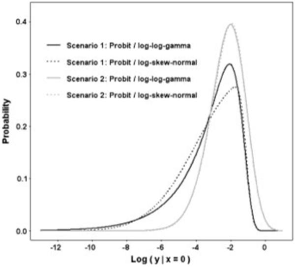
Estimated densities based on the Monte Carlo estimates of 1000 simulated data. True value of q is 2 in Scenario 1 and is 0.5 in Scenario 2.
The average of the estimated standard errors is close to the standard deviation of the parameter estimates in all circumstances, apart from α1, σ,and δ in the case where the true continuous log-error distribution is symmetric. These exceptions are attributable to the singularity of the expected Fisher information matrix at δ=0 [17]. However, the singularity property would not be an issue in regression analysis since accurate estimation of the true intercept and variance, as well as regression parameters, is still attainable. In other words, the issue does not prevent reliable prediction of future observations.
6. CONCLUDING REMARKS
When investigating data that have a fair number of observations at the lower bound of measurement, it is sensible to start by checking whether the percentage of the (possibly transformed) limited responses is consistent with the left tail of a normal distribution. This can be carried out visually through the use of a histogram. Analysis based on a two-part model is recommended should there be evidence of incongruence between the boundary percentage and tail probability. Our efforts in this paper have been focused on modeling the continuous part via the log-skew-normal distribution. Although there are numerous potential candidate distributions, the skewed distribution is intriguing in a number of respects.
The distribution adapts itself to accommodate asymmetry during modeling whenever data possess this characteristic. In other words, it eliminates the need for searching for an ad hoc transformation for normality.
Its regression coefficients (apart from the intercept) have the same interpretation as those in the lognormal model. Thus, the associations between the response and explanatory variables are more directly interpretable than those employing an ‘optimal’ transformation on the response.
Statistical analysis can be easily conducted through the use of existing statistical software programs and standard optimization algorithms.
We have evaluated the MLE using the NLMIXED procedure from the commercial software SAS. A set of good initial values may be crucial to avoid convergence difficulties. They can be chosen by the method of moments or built from the estimates of simpler models. Lin et al. [18] recently considered fitting the skew-normal mixture models using the EM-type techniques. It should be straightforward to adopt their computational routines into our setting.
The assumption of normality after log-transformation on the continuous component can simplify computation but, if incorrect, could contaminate the analytic results. The proposed model shows promise in yielding a significantly better fit than the probit/lognormal model in both censoring and non-censoring cases. However, our empirical study reveals greater discrepancies in inference between the symmetric and skewed models in the presence of censoring. This is perhaps not surprising since the mixing probability and the location of the assumed continuous distribution are unrelated if the data are completely observed, but the assumption of censoring links these components together. Hence if the distribution of the positive observations is skewed to the left (on the log scale) and there is censoring at the lower end of this distribution, we would expect a higher proportion of the limited responses to have come from the continuous part by explicitly accounting for the skewness. Consequently, larger differences between the models could be anticipated on both the mixing probability and the mean of the continuous distribution. We have drawn inferences in our example using both censoring and non-censoring models in order to demonstrate the above claim. It should be noted, however, that a well-specified model should take censoring into account whenever it is known to be present in the data (detection limit), but conversely, the model should not include censoring if censoring is known not to be present.
The likelihood ratio test was used for model selection in this paper, because the normal distribution can be obtained by simply imposing a parameter constraint on the skew-normal distribution. Because the test does not work for non-nested models, one could instead resort to a Bayesian approach in making this judgment. For instance, we could assess the performance of a model using the posterior predictive criteria proposed by Laud and Ibrahim [19]. In particular, censoring could be accommodated into these criteria via a technique similar to that of Gelfand and Ghosh [20], i.e. replace all censored observations with the estimated predictions if the estimated predictive value is smaller than the corresponding censored value. We call attention to the fact that the skew normal family does not lead to fat tails and is therefore unsuitable for predicting extreme outcomes. One could turn instead to the skew-t distribution [11] in this context.
We note finally that the idea of formulating a mixture of two populations to account for the excess of observations at the extreme end has also been well established in other types of dependent variable. The reader is referred to Farewell [21] for an application in survival data (larger than expected long term survivors) and to Bohning et al. [22] for an example implemented on frequency count data (extra zeros).
ACKNOWLEDGEMENTS
The authors thank Dr Patrick F. Sheedy II, MD, Professor of Radiology, Mayo Department of Radiology, and Patricia Peyser, PhD, Professor of Epidemiology, School of Public Health, University of Michigan, for allowing the use of ECAC study data to illustrate the issues and methods discussed in this paper and for valuable suggestions. The data for the ECAC study were collected under NIH grant HL46292. We also thank Iftikhar J. Kullo, MD, Associate Professor of Medicine, Mayo Division of Cardiovascular Diseases, for providing the study subjects of the Functional Arterial Changes in Atherogenesis Study in whom the ECAC study data were analyzed, as well as for reading the manuscript and providing helpful comments.
Contract/grant sponsor: NIH; contract/grant number: HL46292
REFERENCES
- 1.Tobin J. Estimation of relationships for limited dependent variables. Econometrica. 1958;26:24–36. [Google Scholar]
- 2.Cragg JG. Some statistical models for limited dependent variables with application to the demand for durable goods. Econometrica. 1971;39:829–844. [Google Scholar]
- 3.Moulton LH, Halsey NA. A mixture model with detection limits for regression analyses of antibody response to vaccine. Biometrics. 1995;51:1570–1578. [PubMed] [Google Scholar]
- 4.Moulton LH, Halsey NA. A mixed gamma model for regression analyses of quantitative assay data. Vaccine. 1996;14:1154–1158. doi: 10.1016/0264-410x(96)00017-5. [DOI] [PubMed] [Google Scholar]
- 5.Genton MG. Skew-elliptical Distributions and their Applications: A Journey beyond Normality. Chapman & Hall/CRC Press; London: 2004. [Google Scholar]
- 6.Azzalini A. A class of distributions which includes the normal ones. Scandinavian Journal of Statistics. 1985;12:171–178. [Google Scholar]
- 7.Azzalini A. Further results on a class of distributions which includes the normal ones. Statistica. 1986;46:199–208. [Google Scholar]
- 8.John S. The three parameter two-piece normal family of distributions and its fitting. Communications in Statistics—Theory and Methods. 1982;11:879–885. [Google Scholar]
- 9.Mudholkar GS, Hutson AD. The epsilon-skew-normal distribution for analyzing near normal data. Journal of Statistical Planning and Inference. 2000;83:291–309. [Google Scholar]
- 10.Branco MD, Dey DK. A general class of multivariate skew-elliptical distributions. Journal of Multivariate Analysis. 2001;79:99–113. [Google Scholar]
- 11.Sahu SK, Dey DK, Branco MD. A new class of multivariate skew distributions with applications to Bayesian regression models. The Canadian Journal of Statistics. 2003;31:129–150. [Google Scholar]
- 12.Dean EJ. A model trust-region modification of Newton method for nonlinear 2-point boundary-value-problems. Journal of Optimization Theory and Applications. 1992;75:297–312. [Google Scholar]
- 13.Agatston AS, Janowitz WR, Hildner FJ, Zusmer NR, Viamonte M, Jr, Detrano R. Quantification of coronary artery calcium using ultrafast computed tomography. Journal of the American College of Cardiology. 1990;15:827–832. doi: 10.1016/0735-1097(90)90282-t. [DOI] [PubMed] [Google Scholar]
- 14.Kullo IJ, Bielak LF, Turner ST, Sheedy PF, II, Peyser PA. Aortic pulse wave velocity is associated with the presence and quantity of coronary artery calcium: a community-based study. Hypertension. 2006;47:174–179. doi: 10.1161/01.HYP.0000199605.35173.14. [DOI] [PubMed] [Google Scholar]
- 15.Kaufmann RB, Sheedy PF, II, Maher JE, Beilak LF, Breen JF, Schwartz RS, Peyser PA. Quantity of coronary artery calcium detected by electron beam computed tomography in asymptomatic subjects and angiographically studied patients. Mayo Clinic Proceedings. 1995;70:223–232. doi: 10.4065/70.3.223. [DOI] [PubMed] [Google Scholar]
- 16.Prentice RL. A log gamma model and its maximum likelihood estimation. Biometrika. 1974;61:539–544. [Google Scholar]
- 17.Azzalini A, Capitanio A. Statistical applications of the multivariate skew normal distribution. Journal of the Royal Statistical Society, Series B. 1999;61:579–602. [Google Scholar]
- 18.Lin TI, Lee JC, Yen SY. Finite mixture modeling using the skew normal distribution. Statistica Sinica. 2007;17:909–927. [Google Scholar]
- 19.Laud PW, Ibrahim JG. Predictive model selection. Journal of the Royal Statistical Society, Series B. 1995;57:247–262. [Google Scholar]
- 20.Gelfand AE, Ghosh SK. Model choice: a minimum posterior predictive loss approach. Biometrika. 1998;85:1–11. [Google Scholar]
- 21.Farewell VT. The use of mixture models for the analysis of survival data with long-term survivors. Biometrics. 1982;38:1041–1046. [PubMed] [Google Scholar]
- 22.Bohning D, Dietz E, Schlattmann P. The zero-inflated Poisson model and the decayed, missing and filled teeth index in dental epidemiology. Journal of the Royal Statistical Society, Series A. 1999;162:195–209. [Google Scholar]