Quantification and Statistical Modeling—Part I: Breathing-Zone Concentrations of Monomeric and Polymeric 1,6-Hexamethylene Diisocyanate

Abstract

We conducted a repeated exposure-assessment survey for task-based breathing-zone concentrations (BZCs) of monomeric and polymeric 1,6-hexamethylene diisocyanate (HDI) during spray painting on 47 automotive spray painters from North Carolina and Washington State. We report here the use of linear mixed modeling to identify the primary determinants of the measured BZCs. Both one-stage (N = 98 paint tasks) and two-stage (N = 198 paint tasks) filter sampling was used to measure concentrations of HDI, uretidone, biuret, and isocyanurate. The geometric mean (GM) level of isocyanurate (1410 μg m⁻³) was higher than all other analytes (i.e. GM < 7.85 μg m⁻³). The mixed models were unique to each analyte and included factors such as analyte-specific paint concentration, airflow in the paint booth, and sampler type. The effect of sampler type was corroborated by side-by-side one- and two-stage personal air sampling (N = 16 paint tasks). According to paired t-tests, significantly higher concentrations of HDI (P = 0.0363) and isocyanurate (P = 0.0035) were measured using one-stage samplers. Marginal R² statistics were calculated for each model; significant fixed effects were able to describe 25, 52, 54, and 20% of the variability in BZCs of HDI, uretidone, biuret, and isocyanurate, respectively. Mixed models developed in this study characterize the processes governing individual polyisocyanate BZCs. In addition, the mixed models identify ways to reduce polyisocyanate BZCs and, hence, protect painters from potential adverse health effects.

INTRODUCTION

Automotive coatings such as primers, sealers, and clear coats are often based on polyisocyanates of 1,6-hexamethylene diisocyanate (HDI). These formulations consist of trace amounts of HDI monomer and higher amounts of HDI oligomers (e.g. uretidone, biuret, and isocyanurate; Fig. 1) (Janko et al., 1992; Sparer et al., 2004; Fent et al., 2008). During spray painting, polyisocyanates react with polyols to form polyurethane. However, because this reaction is not immediate, overspray in the breathing-zone is likely to contain unreacted polyisocyanates. Diisocyanates are considered a major cause of occupational asthma (Chan-Yeung and Malo, 1995; Bernstein, 1996). Efforts undertaken in the automotive refinishing industry to protect workers from inhalation exposures include replacing semivolatile diisocyanate monomers in the hardener with less volatile diisocyanate oligomers and prepolymers. In addition, workplace health and safety regulations require the use of ventilated booths and respirators during spray painting (Sparer et al., 2004; Pronk et al., 2006). Despite these efforts, painters may still inhale polyisocyanates because of the high levels of diisocyanate oligomers in the painting atmosphere (Janko et al., 1992; Lesage et al., 1992; Rudzinski et al., 1995; Sparer et al., 2004; Pronk et al., 2006). Inadequate protection from respirators due to improper fit, poor maintenance, or insufficient efficiency may also lead to inhalation exposure (Liu et al., 2006).

Fig. 1.

Molecular structures of HDI monomer and its oligomers.

Differences in exposure pathways, biological uptakes, and toxicities among individual polyisocyanates may be expected due to differences in their reactivity, volatility, solubility, and molecular weight. Consequently, exposure assessments designed to understand these differences should characterize exposures to individual polyisocyanates rather than total reactive isocyanate groups (TRIGs). Mathematical modeling may then be used to characterize the processes that govern individual polyisocyanate exposures. An increase in our knowledge and understanding of exposure pathways will help inform strategies to evaluate control technologies and prevent adverse health effects within the occupational environment.

Several deterministic models have been developed for understanding exposures during compressed air spray painting (Carlton and Flynn, 1997a,b; Flynn et al., 1999). However, to our knowledge, only once (Woskie et al., 2004) have statistical methods (i.e. multiple regression) been used to investigate the effects of general process-related variables (i.e. shop size, cars painted per month, etc.) on air concentrations of TRIG. Greater insight may be achieved by using linear mixed modeling (LMM) (Laird and Ware, 1982) to examine the effects of more specific process-related variables (i.e. airflow in the paint booth, volume of the paint booth, etc.) and task-related variables (i.e. paint concentration, paint time, etc.) on air concentrations of individual polyisocyanates. This approach also accounts for random effects associated with the worker and the sampling day or visit and serial correlation of repeated measures.

The objectives of this study were (i) to measure breathing-zone concentrations (BZCs) of HDI monomer and oligomers (i.e. uretidone, biuret, and isocyanurate) during automotive spray painting using a previously published method (Fent et al., 2008) and (ii) to use worker and work environment information to predict exposures and, hence, identify the primary determinants of exposures. To achieve these goals, LMM was applied to evaluate the fixed effects of booth type and covariates upon BZCs of monomeric and polymeric HDI. This work enhances our understanding of the pathways leading to monomeric and polymeric HDI exposures during spray painting and aids to identify the most effective control interventions for reducing those exposures. Furthermore, these models may serve useful for future studies attempting to assign exposures to unsampled workers and/or studies exploring biological uptake and toxicity.

MATERIALS AND METHODS

Recruitment of painters

Automotive spray painters in central North Carolina (NC) and the Puget Sound area of Washington State (WA) were recruited to participate in an exposure-assessment study consisting of air sampling and dermal tape-strip sampling. Letters explaining the study, including potential hazards associated with study participation, were mailed to automotive repair shops in both geographical locations. After ∼2 weeks, phone calls were made to the managers of each shop to gauge interest in participation. If both the manager and the painters expressed interest in the study, visits were made to the respective shops at which time the study was verbally explained and consent forms were provided to the manager and painters.

On the first exposure-assessment visit, the consent form was read to the study subjects and then signed by the participants prior to data collection. Signatures were obtained on subsequent visits if any changes were made to the consent form, but only after thorough explanation of those changes. A total of 15 painters in NC and 32 painters in WA participated in the study. The participation rate was ∼5% in NC and 20% in WA. The higher participation rate in WA was most likely due to the involvement of the WA Department of Labor and Industries (LNI) in the recruitment. Because LNI is a regulatory agency, automotive repair shops with better health and safety practices may have been more likely to participate in the study. In order to assess their exposures, painters were visited on three separate occasions over a 1-year period, with visits at least 1 month apart. Due to attrition, 14 of the 47 painters were visited twice and six painters were visited once.

Data collection and analysis

We attempted to sample exposures during each paint task in which monomeric and polymeric HDI-containing paint was applied (primer, sealer, clear coat, single stage, etc.). A surface coating applied to completion represented one paint task. For example, three coats of clear coat applied to an object or group of objects inside a paint booth constituted one paint task unless the time lapse in between coats was excessively long (i.e. >30 min). The majority (92%) of the sampled paint tasks involved the application of clear coat, which is expected to contain the highest levels of polyisocyanates (Sparer et al., 2004). Isophorone diisocyanate (IPDI) monomers and its oligomers were not analyzed in this study because IPDI-based polyisocyanates are typically present at lower levels than HDI-based polyisocyanates in automotive paint (Woskie et al., 2004). Thus, HDI was the focus of our study.

Personal breathing-zone measurements of each paint task were made using one-stage sampling or two-stage sampling described elsewhere (Fent et al., 2008). The two-stage samplers used in this study contained an untreated polytetrafluorethylene pre-filter (designed to collect diisocyanate aerosols) and a glass–fiber filter impregnated with derivatizing agent (designed to collect and derivatize diisocyanate vapors). The one-stage samplers were identical to the two-stage samplers except that the pre-filter was not included in the cassettes.

Polymerization of polyisocyanates on the untreated pre-filter is possible with two-stage sampling. This problem is expected to be greater the longer the sampling time and more reactive the isocyanate system (Streicher et al., 2000). According to Streicher et al. (1994), two-stage sampling may be an acceptable method in the spray painting environment because HDI-based paints tend to cure slowly and painting tasks typically last <30 min. Because we collected short-term samples (<30 min) and extracted the filters immediately after sampling, we did not expect this potential problem to be a major source of bias. However, evaluation of two-stage samples collected partway through the study showed evidence of such a bias (i.e. low air concentrations relative to high HDI monomer and oligomer paint concentrations). For this reason, we felt it was prudent to begin using one-stage sampling. Consequently, we reasoned that this would also provide a means to compare the performance of one-stage and two-stage samplers both of which are commonly used to monitor atmospheres containing diisocyanates (England et al., 2000).

Table 1 provides a summary of the air sampling scheme used in NC and WA. One- and two-stage sampling was performed in both states. However, two-stage sampling was not performed in WA during the third visit. The number of two-stage samples (N = 198) was more than double the number of one-stage samples (N = 98). In addition, side-by-side one- and two-stage sampling (N = 20) was performed in NC. During the side-by-side sampling, the filter cassettes were attached to the painter's collar and spaced ∼1 inch apart.

Table 1.

Air sampling scheme by state^a

	No. of shops	No. of painters	No. of sampled tasks
			Visit 1	Visit 2	Visit 3	Total
NC	11	15	41	33	21	95
Two stage	11	15	34	26	15	75
One stage	3	3	7	7	6	20
WA	25	32	81	69	51	201
Two stage	24	30	78	45	0	123
One stage	22	25	3	24	51	78

^aFor NC, all one-stage samples were collected simultaneously with two-stage samples. For WA, all one-stage samples were collected independently of two-stage samples.

Directly following the completion of a paint task, one- and two-stage filters were processed by placing the filters in vials containing derivatizing solution. The analytical limits of detection were 2 and 8 fmol μl⁻¹ of derivatizing solution for HDI monomer and oligomers, respectively. More than one air sample was collected if the paint task took >20–30 min. Results were adjusted to time-weighted averages (TWAs) over the painting time for each paint task. Most painters only painted in one type of paint booth; however, four painters did paint in multiple paint booths. On average, 2.4 personal air samples were collected from each painter during a visit. More than one air sample was collected from all but two painters, both of whom painted inside crossdraft booths.

Data were collected on the painters and their work environments for use as potential covariates. Prior to each paint task, samples of the mixed paint were collected for polyisocyanate analysis as described elsewhere (Fent et al., 2008). Airflow inside the paint booth was measured using a rotating vane anemometer (VelociCalc®, TSI, Shoreview, MN, USA) at a perpendicular distance of 10 cm from the return duct. Humidity and temperature inside the paint booths were not consistently recorded. Thus, outdoor relative humidity and temperature were retrieved from a historical database at http://www.wunderground.com and used to estimate the humidity and temperature inside the booths. Because the automotive repair garages did not have air conditioning, the outdoor relative humidity was a reasonable approximation of the indoor humidity. The paint booths, on the other hand, were temperature controlled to ∼24 to 27°C. Making the assumption that the majority of painting took place during the hottest part of the day (12:00 pm to 4:00 pm), temperature during painting was estimated using the maximum outdoor temperature, unless the maximum outdoor temperature was <24°C, in which case a temperature of 23.9°C was assigned to the paint booth. Table 2 summarizes all the variables that were considered in statistical analysis.

Table 2.

Summary of variables used to model concentrations of HDI, uretidone, biuret, and isocyanurate in the breathing-zone of automotive spray painters

Type	Name	Description	Range of values	Mean value	Median value
Classification	Booth typea	Type of ventilated paint booth	Downdraft, semi-downdraft, crossdraft	NA	NA
Continuous	Airflow	Airflow inside the paint booth (m3 min−1)	0–469	221	238
	Booth volume	Volume of the paint booth (m3)	55.3–684	101	95.2
	Experience	Experience spray painting cars (years)	0.25–40	13.4	12
	Humidity	Average relative humidity (%)	39.0–96.0	72.6	74.0
	Paint concentration (HDI)b	Concentration of HDI in paint (mg l−1)	0.014–1060	280	259
	Paint concentration (uretidone)b	Concentration of uretidone in paint (mg l−1)	0.060–20 900	880	68.2
	Paint concentration (biuret)b	Concentration of biuret in paint (mg l−1)	1.00–23 800	2030	814
	Paint concentration (isocyanurate)b	Concentration of isocyanurate in paint (mg l−1)	0.56–357 000	96 000	94 800
	Paint time	Time spent inside the booth painting (min)	1.0–56.0	8.49	6.50
	Temperature	Estimate temperature during spraying (°C)	23.9–33.9	25.0	23.9
	Total time	Total operating time of the sampling pumps (min)	3.0–105	21.4	17.0
Dichotomous	Enclosure	Type of enclosure surrounding the paint booth	1: curtain, 0: wall	0.063	0
	Gun type	Type of spray gun used for applying paint	1: HVLP, 0: conventional	0.92	1
	Paint type	Type of paint applied to the surface of the vehicle	1: clear coat, 0: other	0.92	1
	Sampler type	Type of sampler used to monitor air concentration	1: two stage, 0: one stage	0.66	1

^aBecause booth type is a character variable use for classification, mean and median values could not be calculated (NA = non-applicable).

^bHDI, uretidone, biuret, and isocyanurate were non-detectable in 3.1, 36, 17, and 1.0% of all paint samples, respectively. Multiple imputation (n = 10 imputed datasets) was used to impute paint-sampling data below detection limits.

Statistical analysis

The data were analyzed using SAS 9.1 statistical software (Cary, NC, USA). Due to a relatively high fraction of non-detectable levels of uretidone and biuret (>45%) in air samples, multiple imputation (n = 10 imputed datasets) was used to impute exposure data below detection limits. The logarithmic transformation was taken for all the BZCs and all the paint concentrations except paint concentrations of HDI and isocyanurate, which appeared to follow normal distributions. For these variables, a lower bound of zero was set for the imputations. In order to account for correlations in the multivariate exposure data, we imputed from truncated multivariate normal distributions, with truncation at the limit of detection. Several authors have considered imputation from truncated normal distributions, including Lubin et al. (2004). Our use of a multivariate version of these methods allowed us to control for correlations among like exposures as well as within-subject correlations.

SAS PROC MIANALYZE was used to combine the results of the analyses carried out on the 10 imputed datasets and to obtain valid estimates and statistical inferences. Averages were computed where PROC MIANALYZE could not be used (i.e. marginal R² statistics). The covariates were evaluated for potential collinearity by examining the Spearman correlation coefficients among pairs of covariates. Paint time and total time (r = 0.78) were the only variables to exceed our criterion for high correlation (i.e. r > 0.70) and were only included together in the models if there was evidence that they described separate variability.

LMM (PROC MIXED) was used to investigate the relative influences of fixed effects representing booth type and covariates on BZCs of HDI, uretidone, biuret, and isocyanurate, while accounting for the random effects due to each individual painter and visit day. The general form of the model is provided below:

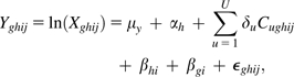for g = 1, 2, …, G visit days; h = 1, 2, …, H booth types; i = 1, 2, …, k_h painters using booth type h; j = 1, 2, …, n_i measurements from painter i in booth type h; and u = 1, 2, …, U covariates in booth type h, where

• X_ghij = polyisocyanate concentration of the jth measurement of the ith painter in the hth booth type during the gth visit day,

• Y_ghij = natural log-transformed value of X_ghij,

• μ_y = intercept,

• α_h = fixed effect for the hth booth type,

• C_ughij = covariate u (or interaction of covariates) for the jth measurement of the ith painter in the hth booth type during the gth visit day,

• δ_u = regression coefficient representing the fixed effect of covariate u,

• β_hi = subject-specific effect of the ith painter in the hth booth type,

• β_ghi = visit-specific effect of the ith painter in the hth booth type during the gth visit, and

• ϵ_ghij = random error of the jth measurement for the ith painter in the hth booth type during the gth visit day.

It is assumed under this model that β_hi, β_ghi, and ϵ_ghij are mutually independent and normally distributed with means of zero and respective variances σ_1,h², σ_2,h², and σ_3,h² representing the between- and within-worker variance components for hth booth type, where total variance σ_y,h² = σ_1,h² + σ_2,h² + σ_3,h² for the hth booth type. It is also assumed that Y_ghij is normally distributed with mean 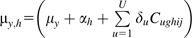and variance σ_y,h².

Candidate covariates were selected by running separate models that considered individual terms and the interaction terms between analyte-specific paint concentration and airflow. From these models, those variables with P-values of <0.15 were used to build final models. Final models were built using a backward elimination procedure in which the least significant variables (P > 0.10) were eliminated one at a time. Insignificant main effects were always retained if their respective interaction terms were significant. To allow for separate parameter estimates for each booth type, interactions between the classification variable booth type and each of the significant variables were evaluated one-at-a-time and retained if the 95% confidence intervals of any two of the parameter estimates did not overlap. To assess model fit, transformed residuals and Malhalanobis’ distance were examined. These diagnostic measures did not identify excessive outliers or problematic observations.

Several R² statistics have been proposed for assessing the goodness of fit of fixed effects (Xu, 2003; Orelien and Edwards, 2008). Marginal R² statistics are more appropriate than conditional R² statistics for estimating explained variability from fixed effects because marginal R² statistics do not use random effects in the computation of predicted means that lead to residuals (Orelien and Edwards, 2008). In this study, a marginal R² statistic proposed by Vonesh and Chinchilli (1997) was used. Orelien and Edwards (2008) found this statistic to perform extremely well at differentiating between full and reduced models and not diverging when models were overfitted. This marginal R² statistic was calculated using simplified mixed models that pooled the within- and between-worker variability among the different booth types and used two dichotomous variables for booth type to account for the fixed effect of booth type (note: readers interested in obtaining the SAS code used for the computations in the paper can contact the corresponding authors directly).

RESULTS

Summary statistics

A summary of BZCs measured by sampler type in NC and WA is provided in Table 3. Because the exposure data were positively skewed, the measures of central tendency and scatter were best described using the geometric mean (GM) and geometric standard deviation, respectively.

Table 3.

BZCs (μg m⁻³) of monomeric and polymeric HDI^a for samples collected in NC and WA stratified by sampler type

Analyte	NC				WA
	Nb	GM	GSD	Range	Nb	GM	GSD	Range
HDI	88	3.21	6.05	0.003–179	200	4.56	5.10	0.0007–65.5
One stage	19	1.54	5.26	0.003–10.7	78	9.49	2.96	0.009–60.3
Two stage	69	3.93	6.00	0.01–179	122	2.85	5.79	0.0007–65.5
Uretidone	88	1.68	27.2	0.002–1430	200	2.35	15.2	0.0004–613
One stage	19	0.84	7.29	0.002–62.6	78	7.02	11.8	0.004–613
Two stage	69	2.04	33.9	0.003–1430	122	1.16	13.8	0.0004–266
Biuret	88	2.58	11.4	0.01–7720	200	12.8	12.4	0.003–1020
One stage	19	3.17	6.07	0.08–70.0	78	24.3	8.22	0.03–1020
Two stage	69	2.44	13.7	0.01–7720	122	8.5	15.3	0.003–734
Isocyanurate	88	958	6.05	4.09–17 800	200	1670	3.96	0.09–18 700
One stage	19	825	4.74	17.8–3190	78	2160	3.67	0.68–18 700
Two stage	69	1000	6.48	4.09–17 800	122	1420	4.06	0.09–14 600

GSD, geometric standard deviation.

^aMultiple imputation (n = 10 imputed datasets) was used to impute air-sampling data below detection limits.

^bNumber of measurements representing the TWA recorded for each paint task. Because of sampling pump malfunction, seven samples collected in NC and one sample collected in WA were excluded.

Other than the side-by-side sampling sets collected in NC, the one- and two-stage samples were collected at different times during the study and, therefore, are not directly comparable. Nevertheless, two-sample t-tests were conducted to explore whether significant differences existed between the sampler types or locations. Two-stage sampling in WA collected significantly higher levels of biuret (P = 0.0019) than did two-stage sampling in NC. One-stage sampling in WA collected significantly higher levels of all the analytes (P ≤ 0.0066) than did one-stage sampling in NC. It should be noted that the one-stage sampling distribution in NC (N = 19) was not sufficiently large or diverse enough (collected from three shops) to make a valid comparison. Irrespective of sampler type, BZCs of biuret and isocyanurate were significantly higher in WA than in NC (P = 0.0044). The effect of location on the results was further evaluated with the statistical modeling.

In WA, one-stage sampling collected significantly higher levels of all the analytes than did two-stage sampling (P ≤ 0.0337). The results of one- and two-stage sampling did not differ significantly in NC except for HDI (P = 0.0434) where two-stage sampling collected more than one-stage sampling, but again, this comparison may not be valid due to the insufficient number and diversity of one-stage samples in NC.

A summary of the air-sampling results by booth type, including restricted maximum likelihood estimates of the within- and between-worker variability, is presented in Table 4. Greater between-worker variability than within-worker variability was observed in BZCs of all polyisocyanates measured in crossdraft booths, but the opposite (i.e. greater within-worker than between-worker variability) was observed for downdraft booths. The GM levels of isocyanurate (1410 μg m⁻³) were higher than all other analytes (i.e. GM ≤ 7.85 μg m⁻³). For all the measured polyisocyanates, GM levels varied considerably among the different booth types with the lowest levels being observed in downdraft booths. This finding may be due in part to differences in the airflows among the booth types as downdraft, semi-downdraft, and crossdraft booths had average airflows of 250, 190, and 102 m³ min⁻¹, respectively. However, after adjusting for airflow in the multivariate models, we observed, on average, higher BZCs in crossdraft or semi-downdraft booths than in downdraft booths for all the measured polyisocyanates (data not shown).

Table 4.

BZCs (μg m⁻³) of monomeric and polymeric HDI^a by type of paint booth

Analyte	Booth type	nb	Nc	Non-detectsd	Summary statistics			REML estimates (logged data)
					GM	GSD	Range	Within-worker variance	Between-worker variance
HDI	Downdraft	31	197	26	2.72	5.74	0.003–48.0	2.23	0.67
	Semi-downdraft	10	60	1	10.1	2.11	0.50–65.5	0.48	0.12
	Crossdraft	10	31	1	9.65	5.58	0.0007–179	0.61	5.18
	All booths	47	288	28	4.10	5.42	0.0007–179	1.78	0.71
Uretidone	Downdraft	31	197	146	1.27	20.7	0.0004–1430	4.60	1.61
	Semi-downdraft	10	60	18	6.96	10.7	0.02–613	0.98	6.92
	Crossdraft	10	31	13	5.39	21.2	0.0007–521	2.89	10.2
	All booths	47	288	177	2.12	20.3	0.0004–1430	3.79	2.90
Biuret	Downdraft	31	197	115	3.46	9.68	0.003–798	3.20	1.70
	Semi-downdraft	10	60	10	44.7	8.23	0.03–734	1.15	4.45
	Crossdraft	10	31	5	49.4	17.1	0.004–7720	2.20	11.0
	All booths	47	288	130	7.85	13.3	0.003–7720	2.78	2.95
Isocyanurate	Downdraft	31	197	2	1210	4.94	0.09–17800	1.98	0.59
	Semi-downdraft	10	60	0	2160	2.08	269–8920	0.29	0.37
	Crossdraft	10	31	1	1600	7.98	0.46–18700	0.64	7.52
	All booths	47	288	3	1410	4.65	0.09–18700	1.66	0.83

GSD, geometric standard deviation; REML, restricted maximum likelihood.

^aMultiple imputation (n = 10 imputed datasets) was used to impute air-sampling data below detection limits.

^bNumber of workers. A total of four painters painted in more than one booth type; two painted in both crossdraft and semi-downdraft booths, one painted in both crossdraft and downdraft booths, and one painted in both semi-downdraft and downdraft booths.

^cNumber of samples. Represents the TWA recorded for each paint task. Of the 296 measurements, eight were excluded due to sampling pump malfunction.

^dNumber of samples collecting non-detectable levels.

Statistical modeling

The mixed models developed for each analyte and booth type are described in Table 5. According to marginal R² statistics, significant fixed effects were able to describe an estimated 25, 52, 54, and 20% of the overall variability in the BZCs of HDI, uretidone, biuret, and isocyanurate, respectively. Analyte-specific paint concentration, airflow, and sampler type were the only variables that were significant in three or more of the models. The effect of changing paint concentration and airflow was evaluated by comparing model predictions where all other variables in the models were assigned median values. These evaluations were performed using models specific to downdraft booths since these booths were the most commonly used booths in this study. As expected, the models predicted increasing BZCs with increasing paint concentrations (Table 6) and decreasing airflow (data not shown). For example, doubling airflow from 200 m³ min⁻¹ (just below the mean) to 400 m³ min⁻¹ (just below the maximum) resulted in ∼40% lower BZC predictions of HDI, biuret, and isocyanurate. However, for the same paint concentration (e.g. 1000 mg l⁻¹), the models predicted higher levels of isocyanurate (2003 μg m⁻³) than any of the other analytes (e.g. biuret = 36.0 μg m⁻³).

Table 5.

Linear mixed models for predicting BZCs^a of HDI, uretidone, biuret, and isocyanurate in automotive spray painters

Covariatesb	HDI (R2 = 0.25)c		Uretidone (R2 = 0.52)c		Biuret (R2 = 0.54)c		Isocyanurate (R2 = 0.20)c
	Parameter estimates (downdraft, semi-downdraft, crossdraft)d	P-valuese	Parameter estimates (downdraft, semi-downdraft, crossdraft)d	P-valuese	Parameter estimates (downdraft, semi-downdraft, crossdraft)d	P-valuese	Parameter estimates (downdraft, semi-downdraft, crossdraft)d	P-valuese
Intercept	1.48, 2.55, 2.24	<0.0001	1.96, 3.10, 2.75	0.0761	−1.69, −0.875, 2.10	0.3127	7.36, 7.90, 7.24	<0.0001
Paint concentration (mg l−1)	0.00207	<0.0001	0.531	<0.0001	0.716	<0.0001	0.0000104	0.0006
Sampler type (1 = two stage, 0 = one stage)	−0.518	0.0105	−0.424	0.0829			−0.300	0.0758
Airflow (m3 min−1)	−0.00260	0.0015			0.00294, 0.00729, −0.0150	0.0727	−0.000457	0.7706
Temperature (°C)			−0.149	0.0280
Paint concentration (mg l−1) × airflow (m3 min−1)					−0.000851	0.0960	−0.00000002467	0.0500
Paint time (min)			0.0297	0.0380
Experience (years painting)					−0.0533	0.0002	−0.0320	0.0059

^aN = 277 (11 of 288 observations were excluded due to missing covariate data).

^bBZCs of all analytes and paint concentrations of dimer and biuret were log-transformed prior to statistical analysis.

^cMarginal R² statistics proposed by Vonesh and Chinchilli (1997).

^dSeparate intercepts were determined for each booth type as specified in the mixed model. Separate covariate parameter estimates were provided for the different booth types if the 95% confidence intervals for any two of the parameter estimates did not overlap.

^eP-values are based on approximate F-tests of fixed effects.

Table 6.

Effect of changing the analyte-specific paint concentrations^a on predicted mean BZCs of each measured polyisocyanate^b in downdraft booths

Paint concentration (mg l−1)	Predicted mean BZC (μg m−3)
	HDI	Uretidone	Biuret	Isocyanurate
10	5.33	3.5	3.4	2021
25	5.50	5.7	5.4	2021
50	5.79	8.2	7.7	2021
100	6.42	11.9	11.0	2022
250	8.76	19.4	17.7	2023
500	14.7	28.0	25.2	2026
1000	41.4	40.4	36.0	2030
2500		65.7	57.6	2044
5000		95.0	82.2	2067
10 000		137	117	2115
25 000				2264
50 000				2537
100 000				3184
250 000				6296

^aPredictions were not made for paint concentrations exceeding the maximum measured paint concentrations of individual monomeric and polymeric HDI.

^bLinear mixed models (Table 5) specific to downdraft booths were used to predict mean BZCs of the logged exposure data (μ_ln). Median values (Table 2) were used for all other covariates in the models. Marginal R² statistics and total variance estimates (σ_ln²) for the analytes measured in downdraft booths were used to compute arithmetic means (μ_x) with the following formula: .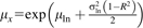

Because sampler type was a significant predictor of BZC in the HDI, uretidone, and isocyanurate models, paired t-tests were conducted on the results of side-by-side one- and two-stage sampling (N = 16 paint tasks). Four side-by-side sets of samples were excluded from the analysis due to sampling pump malfunction. In comparison to two-stage samplers, one-stage samplers measured significantly higher levels of HDI (mean difference = 1.28 μg m⁻³, P = 0.0363) and isocyanurate (mean difference = 673 μg m⁻³, P = 0.0035). Insignificant differences between one- and two-stage samplers were observed for the analytes biuret (mean difference = 4.98 μg m⁻³, P = 0.0652) and uretidone (mean difference = −36.0 μg m⁻³, P = 0.1380). It should be noted that out of the 16 one- and two-stage sampling sets for the analytes HDI, uretidone, biuret, and isocyanurate, 2, 13, 8, and 0 of the samples were below the limit of detection, respectively.

Location (NC versus WA) was not a significant predictor (P ≤ 0.4088) in any of the final mixed models, indicating that differences in BZCs between NC and WA (Table 3) were adequately explained by the significant fixed effects, such as paint concentration or sampler type. According to Akaike information criteria, using visit day as a random effect significantly improved the fit of the final models, suggesting that intervisit variability was not adequately explained by the significant fixed effects.

DISCUSSION

Personal air samples were collected from 47 automotive spray painters in this study, thereby providing estimates of BZCs of monomeric and polymeric HDI in the automotive refinishing industry. Using quantitative inhalation exposure and covariate data in LMM, we identified the primary determinants of BZCs of HDI, uretidone, biuret, and isocyanurate. However, there were several limitations in this study that were taken into consideration when we evaluated the results.

First, although IPDI may be an important constituent of some automotive coatings, we did not analyze for IPDI or its oligomers in this study. Thus, our estimates of exposure do not capture all polyisocyanates of concern. Second, because the one- and two-stage samples were collected at different times during the study, they are not directly comparable. Last, >40% of the uretidone and biuret data were below detection limits. Consequently, statistical power was reduced for the analyses of the uretidone and biuret data. However, multiple imputation was used for BZCs below the detection limits in an effort to obtain better estimates of the parameters of interest (Lubin et al., 2004).

The mixed models developed in this study described more than half the variability in BZCs of uretidone and biuret (R² > 50%) and lesser variability in BZCs of HDI and isocyanurate (R² ≥ 20%). Marginal R² statistics calculated for models specific to each booth type and analyte (data not shown) were highly variable, ranging from 0.05 for isocyanurate exposure in semi-downdraft booths to 0.79 for biuret exposure in semi-downdraft booths. Low R² values (i.e. <0.20) may partially reflect the lack of between-worker variability in the respective exposure distributions (between-worker variability is generally easier to characterize than within-worker variability). Nevertheless, the large range of marginal R² values among the different booth types for analyte-specific models suggest that the processes governing BZCs are different for the different booth types. Thus, classification of the mixed models by analyte and booth type is appropriate.

Although unique models were built for each measured polyisocyanate, analyte-specific paint concentration, airflow, and sampler type were significant predictors in three or more of the models. In addition, the interaction between paint concentration and airflow was significant in the biuret and isocyanurate models, suggesting that the relationship between paint concentration and BZC depends on the airflow in the booth. Expectations are that higher analyte-specific paint concentrations will lead to higher BZCs while increased airflow will lead to lower BZCs of each polyisocyanate. This was observed in the model predictions in which changing analyte-specific paint concentration and airflow were evaluated. Unexpectedly, using the same analyte-specific paint concentration, the models predicted higher BZCs of isocyanurate than any of the other analytes (Table 6). The most likely reason for this finding is that the isocyanurate model overpredicted BZCs at lower levels of paint concentrations due to the fact that 90% of the paint concentrations used to generate the model were between 10 900 and 195 000 mg l⁻¹. In fact, significant differences between predicted means and actual values were observed when the actual values were below the 10% quantile (∼270 μg m⁻³), and it was evident that paint concentration <10 000 mg l⁻¹ had a negligible effect on isocyanurate BZC (Table 6). Despite this limitation, the isocyanurate model performed well in terms of prediction (i.e. 90% of the predictions within ±2 scaled residuals) and, therefore, provides reasonable estimates of central tendency for most of the data collected in this study. We believe that the predictions of oligomer BZCs at respective paint concentrations of 10 000 mg l⁻¹ by these models are valid and, as such, demonstrate the differences between isocyanurate and the other oligomer concentrations in these spray painting operations (Table 6).

Another possibility for these differences is that the analysis of paint samples underestimated the true concentration of isocyanurate in the paint. The interquartile range of isocyanurate paint concentration was 45 000 to 135 000 mg l⁻¹, representing ∼3.0 to 8.5% of the paint formulation. According to the material safety data sheets (PPG, 2009a,b,c) of some of the most common hardeners used in the workplace and assuming a hardener to coating ratio of 4:1, the proportion of polymeric HDI is expected to range from 2.5 to 20%. Thus, measurements of isocyanurate in paint are within the expected range.

Assuming that the mixed models accurately represent conditions in the atmosphere, differences in reactivity could explain the differences in the predicted mean BZCs (Table 6). For example, HDI, uretidone, and biuret may polymerize more rapidly in the atmosphere than isocyanurate. In contrast, isocyanurate could react more rapidly and completely with the derivatizing agent than the other polyisocyanates. Moreover, isocyanurate may be formed during the polymerization process as other polyisocyanates react with each other. The significant effect of temperature in the uretidone model may be indicative of increasing reactivity with increasing temperature. In fact, uretidone may be the most reactive polyisocyanate measured in this study due to the strained configuration of its four-member ring.

Reactivity of polyisocyanates is probably the reason why the effect of sampler type was significant in the HDI, uretidone, and isocyanurate models. Two-stage samplers may underestimate BZCs of reactive polyisocyanates due to polymerization of polyisocyanates on the untreated pre-filter of the sampler. This problem may be avoided by using one-stage samplers onto which all polyisocyanates are simultaneously collected and derivatized on one filter. Thus, higher BZCs may be measured when one-stage samplers are used instead of two-stage samplers.

Because two-stage samplers were used for the first part of this study and one-stage samplers were used for the second part of this study, observed differences could be due to variable differences between the first and second parts of the study (i.e. selection bias). However, we controlled for many of these variables (airflow, temperature, etc.) by including them in the LMM. Furthermore, the significant effect of sampler type was corroborated by paired two-sample t-tests comparing side-by-side sets of one- and two-stage samplers in which significant differences were observed for the analytes HDI (P = 0.0363) and isocyanurate (P = 0.0035). Thus, it is likely that the observed differences between one- and two-stage sampling results for HDI and isocyanurate are due to differences in the design of the samplers. Significant differences were not observed between one- and two-stage sampling for uretidone and biuret. It is possible that significant differences were not detected because of insufficient statistical power due to the large proportion of non-detectable measurements or because of reactivity differences among the different polyisocyanates. Further investigation is needed to evaluate the reactivity of the different polyisocyanates in the painting atmosphere and implications of this reactivity on human health endpoints such as tissue absorption and respiratory sensitization.

Comparison of one- and two-stage sampling results in NC (Table 3) seems to contradict our findings that suggest a two-stage sampling bias. However, only 19 one-stage samples were collected in NC. In addition to the lack of statistical power, the three shops that were sampled with one-stage samplers may not be representative of all the automotive repair shops in the study. It is possible that the paint being used in these three shops was rapidly curing and thereby resulted in lower measured concentrations due to polymerization on the air filters. Even one-stage samplers can underestimate concentrations in atmospheres containing rapidly curing isocyanates (Streicher et al., 2000). Furthermore, these three shops appeared to have been better controlled than the other shops in NC. Downdraft booths were used in 18 of the 20 paint tasks with an average airflow of 261 m³ min⁻¹ compared to the other shops in NC where downdraft booths were used in 39 of 55 paint tasks with an average airflow of 204 m³ min⁻¹. Moreover, the one-stage samplers in question were collected simultaneously with the two-stage samplers and these two-stage samplers measured significantly lower concentrations of HDI and isocyanurate.

A time-dependent decrease in sampling efficiency has been shown for long-term filter sampling of atmospheres containing toluene diisocyanate (Sennbro et al., 2004). The variables, paint time, and total time (or sampling time) were evaluated in the mixed models. Total time was not significant in any of the models and paint time was significant only in the uretidone model. If uretidone was polymerizing over time, we would expect paint time to have a negative parameter estimate, but instead, paint time had a positive parameter estimate. The significant effect of paint time may simply represent the accumulation of uretidone aerosols in the atmosphere over time. Because total time (or sampling time) was not significant in the models, a time-dependent decrease in sampling efficiency for these short-term samples either did not exist or was negligible. Another possibility is that the effect of sampling time was unobservable (i.e. polymerization happened immediately) for rapidly curing polyisocyanates.

Experience (i.e. years painting) was a significant variable in both the biuret and the isocyanurate models in which more experience was associated with lesser exposure. Flynn et al. (1999) found that the painter orientation relative to the direction of the airflow played a significant role in affecting BZCs in crossdraft booths. It is likely that more experienced painters received less exposure to biuret and isocyanurate because they produce less overspray or position their bodies to avoid overspray. Consequently, training automotive spray painters on the best techniques for applying paint may help reduce personal exposures.

In comparison to our mixed models, Woskie et al. (2004) developed a multiple regression model to predict BZC's of TRIG. Significant covariates in this model included: volume of polyisocyanates applied, volume of clear coat used per month, and type of paint booth. These general process-related variables described an estimated 39% of the variability in the BZCs of TRIG, which is within the range of variability (20–54%) described by our analyte-specific models. Because the models generated in our study used specific process- and task-related variables, it is difficult to compare our models to the model developed by Woskie et al. (2004). Nevertheless, our models may be more practical in terms of identifying practices and control technologies to reduce personal exposures.

In addition to statistical models, deterministic models have been used to understand exposures during spray painting. Among the most notable in the literature is the model developed by Flynn et al. (1999) for predicting BZCs of general aerosols during spray painting in crossdraft booths. In addition to painter orientation, the most important parameters of this model were generation rate, momentum flux of air from gun, and momentum flux of air to worker's body. Although these parameters were not directly measured in our study, generation rate may depend on the concentrations of polyisocyanates in paint, momentum flux of air from gun likely depends on the type of spray gun being used, and momentum flux of air to painter's body may depend on the airflow in the booth. These variables, except for gun type, were significant in three or more of the mixed models, and it is probable that gun type would have been significant had there been more variability in gun type (i.e. high volume, low pressure guns were used in 92% of the paint tasks). It is important to note, however, that airflow had a protective effect even in crossdraft booths. Thus, airflow in this study generally functioned to draw overspray away from the painter's body rather than toward the painter's body. Flynn et al. (1999) determined that momentum flux of air from the gun was important as it affected the amount of aerosol ‘bounce back’ into the breathing zone. The size of object being sprayed, angle of spray gun relative to the object, and distance between spray gun and object are also important factors involved in ‘bounce back’ but were not recorded in this study due to the difficulty in measuring such factors.

The random effect of visit day was significant in all the final mixed models. This suggests that BZCs are likely to vary from visit to visit due to factors other than those which were evaluated in this study. Varying work practices are probably a major cause of the intervisit variability. Work practices may depend on a number of factors such as the size and orientation of the objects being painted, the busyness of the shop, and the condition of the work equipment. The intervisit variability observed in this study underscores the importance of collecting samples at different times of the year in order to obtain the most representative exposure estimates.

The BZCs reported in this paper (Tables 3 and 4) represent task-based (≤30 min) TWAs. Thus, ceiling limits or short-term exposure limits (STELs) are more appropriate for comparison than work-shift (i.e. 8-h TWA) exposure limits. The National Institute for Occupational Safety and Health ceiling limit for HDI (i.e. 140 μg m⁻³) was exceeded only once (i.e. 179 μg m⁻³) during this exposure-assessment study. This is not surprising since HDI represented <1% of all polyisocyanates in the automotive paint. Oregon is the only government entity in the USA to promulgate a STEL for HDI-based polyisocyanates biuret and isocyanurate (i.e. 1 mg m⁻³). The BZCs measured in this study are not directly comparable to the Oregon STEL because they were not time weighted over 15 min. Nevertheless, it is interesting to note that the Oregon STEL was exceeded by 71% of the task-based BZCs, with the highest isocyanurate BZC (18 700 μg m⁻³) being over 18 times greater than the recommended limit.

In a 1980–1990 survey of Oregon automotive repair shops, Janko et al. (1992) measured a GM of 14 μg m⁻³ for HDI and 1600 μg m⁻³ for HDI-based polyisocyanates, with respective peak concentrations of 340 and 18 400 μg m⁻³. Similar levels of biuret and isocyanurate combined (GM = 1470, peak = 19 700 μg m⁻³) and lower levels of HDI (GM = 4.1, peak = 179 μg m⁻³) were measured in our study. It is important to note that painters in this study were protected by respirators of various types (i.e. half face, powered air purifying, supplied air, etc.). Over 70% of the painters wore half-face respirators equipped with organic vapor cartridges. The Occupational Safety and Health Administration (OSHA) assigned protection factor for half-face respirators is 10 (OSHA, 2006). After accounting for the OSHA protection factor (i.e. dividing the BZCs by 10), we observed that >5% of the task-based BZCs exceeded the Oregon STEL. Liu et al. (2006) found that the average workplace protection factor for half-face respirators equipped with organic vapor cartridges was 388 for polymeric HDI. Such protection would reduce the inhaled portion of the highest isocyanurate concentration to ∼50 μg m⁻³. Although well below the Oregon STEL, this level of exposure could still pose health risks to susceptible or sensitized individuals. This underscores the importance of reducing air concentrations inside the paint booths.

The analyte-specific mixed models we developed (Table 5) share some important similarities. Three variables (i.e. analyte-specific paint concentration, airflow, and sampler type) were common to three or more of the mixed models. According to the model predictions, reducing analyte-specific paint concentrations and/or increasing airflow results in lower BZCs of polyisocyanates. In addition, lower BZCs of all polyisocyanates were measured in downdraft booths than crossdraft or semi-downdraft booths, which is consistent with previous findings of particulate levels in paint booths (Heitbrink et al. 1995). Although painters and shop managers have limited control over polyisocyanate concentrations in the paint and the type of paint booth installed in the workplace, airflow inside the paint booth can be maximized by changing supply and return air filters on a regular basis and ensuring that plastic sheeting and masking tape are not obstructing the return ducts. These simple acts of maintenance and prevention could have tremendous implications on the health and safety of automotive spray painters.

A significant finding from this study was the effect of sampler type on measured BZCs of HDI and isocyanurate in short-term samples (<30 min). Because the two-stage samplers appeared to underestimate the air concentrations of HDI and isocyanurate in short-term samples in this study, investigators should carefully consider the type of sampler to use for task-based monitoring of reactive compounds like polyisocyanates. The mixed models we developed may provide a reasonable way of estimating worker exposure in retrospective studies where air-sampling data is lacking but where the other covariates can be adequately estimated. However, validation of these models is necessary to confirm their usefulness for exposure reconstruction.

FUNDING

National Institute for Occupational Safety and Health (R01-OH007598, T42/CCT422952, T42 OH008673); National Institute of Environmental Health Sciences (P30ES10126, T32 ES007018); American Chemistry Council (RSK0015-01).

References

- Bernstein JA. Overview of diisocyanate occupational asthma. Toxicology. 1996;111:181–9. doi: 10.1016/0300-483x(96)03375-6. [DOI] [PubMed] [Google Scholar]
- Carlton GN, Flynn MR. Field evaluation of an empiracle-conceptual exposure model. Appl Occup Environ Hyg. 1997a;12:555–61. [Google Scholar]
- Carlton GN, Flynn MR. A model to estimate worker exposure to spray paint mists. Appl Occup Environ Hyg. 1997b;12:375–82. [Google Scholar]
- Chan-Yeung M, Malo JL. Occupational asthma. N Engl J Med. 1995;333:107–12. doi: 10.1056/NEJM199507133330207. [DOI] [PubMed] [Google Scholar]
- England E, Key-Schwartz R, Lesage J, et al. Comparison of sampling methods for monomer and polyisocyanates of 1,6-hexamethylene diisocyanate during spray finishing operations. Appl Occup Environ Hyg. 2000;15:472–8. doi: 10.1080/104732200301250. [DOI] [PubMed] [Google Scholar]
- Fent KW, Jayaraj K, Ball LM, et al. Quantitative monitoring of dermal and inhalation exposure to 1,6-hexamethylene diisocyanate monomer and oligomers. J Environ Monit. 2008;10:500–7. doi: 10.1039/b715605g. [DOI] [PubMed] [Google Scholar]
- Flynn MR, Gatano BL, McKernan JL, et al. Modeling breathing-zone concentrations of airborne contaminants generated during compressed air spray painting. Ann Occup Hyg. 1999;43:67–76. [PubMed] [Google Scholar]
- Heitbrink WA, Wallace ME, Bryant CJ, et al. Control of paint overspray in autobody repair shops. Am Ind Hyg Assoc J. 1995;56:1023–32. doi: 10.1080/15428119591016467. [DOI] [PubMed] [Google Scholar]
- Janko M, McCarthy K, Fajer M, et al. Occupational exposure to 1,6-hexamethylene diisocyanate-based polyisocyanates in the state of Oregon, 1980–1990. Am Ind Hyg Assoc J. 1992;53:331–8. doi: 10.1080/15298669291359735. [DOI] [PubMed] [Google Scholar]
- Laird NM, Ware JH. Random-effects models for longitudinal data. Biometrics. 1982;38:963–74. [PubMed] [Google Scholar]
- Lesage J, Goyer N, Desjardins F, et al. Workers’ exposure to isocyanates. Am Ind Hyg Assoc J. 1992;53:146–53. doi: 10.1080/15298669291359410. [DOI] [PubMed] [Google Scholar]
- Liu Y, Stowe MH, Bello D, et al. Respiratory protection from isocyanate exposure in the autobody repair and refinishing industry. J Occup Environ Hyg. 2006;3:234–49. doi: 10.1080/15459620600628704. [DOI] [PubMed] [Google Scholar]
- Lubin JH, Colt JS, Camann D, et al. Epidemiologic evaluation of measurement data in the presence of detection limits. Environ Health Perspect. 2004;112:1691–6. doi: 10.1289/ehp.7199. [DOI] [PMC free article] [PubMed] [Google Scholar]
- Orelien JG, Edwards LJ. Fixed-effect variable selection in linear mixed models using R2 statistics. Comput Stat Data Anal. 2008;52:1896–907. [Google Scholar]
- OSHA. Occupational safety and health standards, personal protective equipment, respiratory protection. Occupational Health and Safety Administration; 2006. 29 CFR 1910.134. Washington, DC. [Google Scholar]
- PPG. Material safety data sheet, Deltron medium temperature activator, DCH2084. 2009a. Available at https://corporateportal.ppg.com/NA/Refinsh/PPGRefinsh/EN. Accessed June 2009. [Google Scholar]
- PPG. Material safety data sheet, Deltron mid temperature hardener, DCH3085. 2009b. Available at https://corporateportal.ppg.com/NA/Refinsh/PPGRefinsh/EN. Accessed June 2009. [Google Scholar]
- PPG. Material safety data sheet, global refinishing medium hardener, D8280. 2009c. Available at https://corporate. Accessed June 2009. [Google Scholar]
- Pronk A, Tielemans E, Skarping G, et al. Inhalation exposure to isocyanates of car body repair shop workers and industrial spray painters. Ann Occup Hyg. 2006;50:1–14. doi: 10.1093/annhyg/mei044. [DOI] [PubMed] [Google Scholar]
- Rudzinski WE, Dahlquist B, Svejda SA, et al. Sampling and analysis of isocyanates in spray-painting operations. Am Ind Hyg Assoc J. 1995;56:284–9. doi: 10.1080/15428119691014422. [DOI] [PubMed] [Google Scholar]
- Sennbro CJ, Ekman J, Lindh CH, et al. Determination of isocyanates in air using 1-(2-methoxyphenyl)piperazine-impregnated filters: long-term sampling performance and field comparison with impingers with dibutylamine. Ann Occup Hyg. 2004;48:415–24. doi: 10.1093/annhyg/meh035. [DOI] [PubMed] [Google Scholar]
- Sparer J, Stowe MH, Bello D, et al. Isocyanate exposures in autobody shop work: the SPRAY study. J Occup Environ Hyg. 2004;1:570–81. doi: 10.1080/15459620490485909. [DOI] [PubMed] [Google Scholar]
- Streicher RP, Kennedy ER, Lorberua CD. Strategies for the simultaneous collection of vapors and aerosols with emphasis on isocyanate sampling. Analyst. 1994;119:89–97. doi: 10.1039/an9941900089. [DOI] [PubMed] [Google Scholar]
- Streicher RP, Reh CM, Key-Schwartz RJ, et al. Determination of airborne isocyanate exposure: considerations in method selection. Am Ind Hyg Assoc J. 2000;61:544–56. doi: 10.1080/15298660008984567. [DOI] [PubMed] [Google Scholar]
- Vonesh EF, Chinchilli VM. Linear and nonlinear models for the analysis of repeated measurements. New York, NY: Marcel Dekker; 1997. [Google Scholar]
- Woskie SR, Sparer J, Gore RJ, et al. Determinants of isocyanate exposures in auto body repair and refinishing shops. Ann Occup Hyg. 2004;48:393–403. doi: 10.1093/annhyg/meh021. [DOI] [PubMed] [Google Scholar]
- Xu R. Measuring explained variation in linear mixed effects models. Stat Med. 2003;22:3527–41. doi: 10.1002/sim.1572. [DOI] [PubMed] [Google Scholar]