Tensor Splines for Interpolation and Approximation of DT-MRI With Applications to Segmentation of Isolated Rat Hippocampi

Abstract

In this paper, we present novel algorithms for statistically robust interpolation and approximation of diffusion tensors—which are symmetric positive definite (SPD) matrices—and use them in developing a significant extension to an existing probabilistic algorithm for scalar field segmentation, in order to segment diffusion tensor magnetic resonance imaging (DT-MRI) datasets. Using the Riemannian metric on the space of SPD matrices, we present a novel and robust higher order (cubic) continuous tensor product of B-splines algorithm to approximate the SPD diffusion tensor fields. The resulting approximations are appropriately dubbed tensor splines. Next, we segment the diffusion tensor field by jointly estimating the label (assigned to each voxel) field, which is modeled by a Gauss Markov measure field (GMMF) and the parameters of each smooth tensor spline model representing the labeled regions. Results of interpolation, approximation, and segmentation are presented for synthetic data and real diffusion tensor fields from an isolated rat hippocampus, along with validation. We also present comparisons of our algorithms with existing methods and show significantly improved results in the presence of noise as well as outliers.

I. Introduction

Analysis of matrix-valued image data is becoming quite common as advances in imaging technology allow for the collection of matrix-valued datasets. In medical imaging, in the last decade, it has become possible to collect magnetic resonance imaging (MRI) data that can be used to infer the apparent diffusivity of water in tissue in vivo. A rank 2 tensor has been commonly used to approximate the diffusivity profile at each lattice point of the image lattice [1]. This approximation yields a diffusion tensor magnetic resonance imaging (DT-MRI) dataset that is a matrix-valued image. These tensors are elements of the space of the (3 × 3) positive-definite matrices denoted by P(3). A word on terminology, the space of symmetric positive definite (SPD) rank 2 tensors describes the space of all SPD matrices and in general, we use the notation P(n) to denote the space of SPD matrices of size (n, n). In this paper, we will be concerned only with rank 2 tensors and for brevity, we will drop the term rank 2 and simply use the word tensors to imply rank 2 tensors. Mathematically, these positive definite diffusion tensors belong to a Riemannian symmetric space [2], where the Riemannian metric is defined by the inner product assigned to each point of this space. By using this metric, one can compute geodesic (shortest) distances between the points (diffusion tensors) of this space and compute various statistics in this space [3]–[8].

Processing of DT-MRI datasets has scientific significance in clinical sciences. Most of these applications involve processing that more often than not involves interpolation of the diffusion tensor fields. For example, registration of DT-MRI datasets will require interpolation to be employed when a registration transformation is applied to a tensor field defined on a lattice. Other examples that require tensor field approximation as well as interpolation include tensor field segmentation, atlas construction, etc.

In this paper, we present a novel diffusion tensor field approximation algorithm. Our algorithm approximates and interpolates the diffusion tensor fields by forming a higher order continuous tensor product of B-splines using the Riemannian metric on the space of SPD matrices. Our method involves a two-step procedure wherein the first step uses Riemannian distances to evaluate a tensor spline by computing a weighted intrinsic average of tensors and the second step minimizes the Riemannian distance between the evaluated tensor spline and the given data. Furthermore, we present a novel DT-MRI multimodal (multiclass regions) segmentation algorithm using the proposed tensor splines as an approximation module. The segmentation is achieved by jointly estimating the label (assigned to each tensor residing at a voxel) field and the parameters (control points) of each smooth tensor spline model representing the labeled regions. The label field is modeled by a Gauss Markov measure field (GMMF) and the segmentation algorithm very efficiently computes the posterior marginal probability distribution of the label field (given the parameters describing the region model) as the global minimizer of a linearly constrained quadratic energy.

We present comparisons of our algorithms with existing methods applied to synthetically generated diffusion MRI data, and show significantly improved results in the presence of noise and outliers. We also present several 3-D DT-MRI approximation and segmentation results from an isolated rat hippocampus. The motivation for segmenting and analyzing the hippocampus is due to its importance in semantic and episodic formation that is particularly vulnerable to acute or chronic injury [9], [10]. In current clinical practice, we only look at the whole hippocampus and describe atrophy for epilepsy (hippocampal sclerosis), schizophrenia, depression, hypoxia-ischemia, trauma, and Alzheimer’s disease and other dementias. Obviously, these cannot be distinguished from each other and hippocampal atrophy is a late imaging sign of pathology. However, we know from more than 100 years of literature that the hippocampus is made of many different cytoarchitectural regions and that these regions are selectively vulnerable to the aforementioned diseases (e.g., the CA1 and subicular regions are affected by Alzheimer’s disease while the dentate gyrus is affected by medial temporal lobe epilepsy). These regions can be distinguished by diffusion tensor MRI. Thus, the segmenting techniques being developed here could prove useful to improving the sensitivity and specificity of diffusion MRI for detecting and monitoring hippocampal diseases. We can also use these methods for studies in animal models of hippocampal disease. Structural insights from high-resolution DT-MRI imaging of the isolated rat hippocampus were presented previously [11]. In our experiments, we use these structural results [11] for validation of the obtained segmentation.

In the following sections, we review several existing methods for tensor field interpolation/approximation and segmentation. Section II contains the mathematical preliminaries on geometry of the space of diffusion tensors that will be used in developing the interpolation and approximation algorithms. In Section III, we present the tensor splines interpolation and approximation algorithms. Section IV contains the application of these algorithms as a module in a tensor field segmentation algorithm. Section VI contains the discussion and conclusion.

A. Tensor Field Interpolation and Approximation

Directly performing smooth interpolation of the individual components of the diffusion tensor matrices [12] does not preserve most of the properties, e.g., the value of the determinant of the diffusion tensors, etc. This motivates us to seek alternative methods to achieve interpolation/approximation and segmentation. Smooth interpolation of orientation fields has been proposed in [13]. Although rank-2 tensors contain the notion of orientation (e.g., the orientation of its eigenvectors), their structure is much more complicated. Wang and Vemuri [4], [5] used the symmetrized Kullback–Liebler (KL) divergence as a “distance” measure between two SPD tensors. They also derived a closed form solution for computing the mean of two or more SPD tensors. This result can be used in the context of interpolation and approximation of SPD tensors but this aspect was never explored. In [3], [14], and [15], a Riemannian metric was proposed for geodesic distance computation between two tensors. However, none of these methods on geodesic curve computation between tensors use higher order smoothness constraints in achieving the interpolation/approximation. Thus, although there is continuity of the interpolated dataset, higher order continuity and hence smoothness is lacking. Recently, a log-Euclidean metric was proposed in [16] for computing with tensors. In this work, the elements from the space of positive definite diffusion tensors, P(3), are mapped to their tangent space, denoted by Sym(3), using the matrix logarithm map. The tangent space of P(3) forms a vector space of dimension 6. Therefore, one can use the Euclidean norm for computations in this tangent space and finally by using the inverse mapping, the interpolated data are mapped back to the space of positive definite matrices P(3). This framework is very interesting and has advantages due to its high computational efficiency. Approximation of matrix-valued images can be achieved via various regularization methods. For instance, a PDE-based approach as was proposed in [17]. Another tensor field regularization method was proposed in [18] using normalized convolution and Markov random fields (MRFs) in a Bayesian framework. The SPD tensors are treated as vectors in 6-D and their components are treated independently. Most of the aforementioned methods disregard the special geometry of the space of SPD diffusion tensors in the regularization, which in turn may lead to inaccurate predictions (e.g., wrong determinants, lack of affine invariance, etc.).

Affine invariance is a desirable feature for segmentation algorithms to possess. Many a time, when a patient being imaged moves, the image data undergo rigid motions; moreover, if there are breathing artifacts, data undergo an affine deformation. Other scenarios include pre- and the post-surgical DT-MRI data acquired from the same patient, data acquired over time depicting tumor growth, etc. In these latter situations, the diffusivity of the underlying tissue microstructure is altered and does not remain constant. The true transformation of the diffusivity is actually unknown and an affine transformation is at best an approximation. Under these conditions, it is desirable to have affine invariance of the segmented structures, i.e., the segmentations of the two images should be related by the same affine transform that the two images are related by.

In [19], it was shown that, under the assumption of tissue microstructure remaining intact between two data acquisitions, the diffusion tensors are always transformed (pre- and post-multiplication) only by rotations regardless of the order of the transformation relating the two image coordinate systems. This is certainly true for the case when there is a rigid motion of the patient between the two acquisitions. However, there are many applications that do not guarantee this condition and the research reported here is an attempt to address this problem through the imposition of an affine invariance requirement on the segmentation. The claim is that if the relationship between the two image’s coordinate systems denoted by X and Y can be approximated by an affine transform, the diffusion tensors estimated from each image would be related by T_Y = A^tT_XA, where T_X and T_Y denote the tensor fields on the coordinate systems X and Y, respectively. This is mathematically precise and would hold when there are microstructural changes that can be approximated by affine transforms. For more details on affine invariant segmentation, the reader is referred to [5].

B. Tensor Field Segmentation

In this section, we will briefly review SPD tensor field segmentation algorithms. In [20], Zhukov et al. proposed a level set segmentation method that segments the scalar anisotropic property computed from the diffusion tensor. By using such a scalar field, the direction information contained in the tensor field has been ignored. Thus, such a method will fail to correctly segment two homogeneous regions of a tensor field that have the same scalar anisotropy property but are oriented in different directions. Feddern et al. [21] extended the mean curvature flow and self-snakes models to matrix-valued data. However, their method employs the Euclidean metric to measure distance between tensors and not the Riemannian metric discussed earlier. Thus, it does not possess some of the interesting properties that accrue from the use of a Riemannian framework (e.g., the affine invariance property, etc.). Wang et al. [4] developed a region-based active contour model for tensor field segmentation. They generalized the well known region-based active contour model for scalar field segmentation to that of tensor fields, and developed a variational principle using the Forbenius norm of the difference of tensors as a discriminant in the data term. More recently, Lenglet et al. [15] developed a statistical surface evolution framework using the Fisher-Rao metric. They employed the principle that within a region the diffusion tensors can be modeled by using statistics and distributions of diffusion tensors. The surface evolution framework and the active contour models can be extended to cope with multiple types of regions, but such an extension is computationally expensive and can be quite cumbersome.

II. Mathematical Preliminaries

In this section, we briefly review the geometry of the space of diffusion tensors. More detailed expositions on some of this material may be found in [3], [6], and [7].

The space of rank 2 diffusion tensors can be viewed as a Riemannian symmetric space [22], where a Riemannian metric assigns an inner product to each point of this space. By using this metric, we can compute geodesic distances between diffusion tensors and calculate statistics on this space [3], [6], [7]. For example, the mean tensor of a set of diffusion tensors can now be computed as that tensor that minimizes the sum of squared Riemannian distances between itself and the given set of tensors. The mean tensor may be employed as an interpolant for performing principal geodesic analysis, etc.

In the aforementioned Riemannian framework, the distance between two tensors T₁ and T₂ is given by dist² (T₁, T₂) = trace(log(T₁^−1/2T₂T₁^−1/2)²), where log is the matrix logarithm operation. By using this distance measure, the geodesic curve (shortest path) between T₁ and T₂ is defined uniquely. The tangent, specified at the first tensor with respect to the other one along the unique geodesic between them, is a 3×3 symmetric matrix and is given by the Riemannian-log map, Log_T1(T₂) = T₁^1/2 log(T₁^−1/2T₂T₁^−1/2)T₁^1/2. The inverse operation is given by the Riemannian-exp map, Exp_T1(T) = T₁^1/2exp(T₁^−1/2TT₁^−1/2)T₁^1/2, where Exp is the matrix exponential operation and T is a 3 × 3 symmetric matrix. We will use this Riemannian distance between SPD tensors in computing the distance between the given data and the tensor spline approximation of the data as well as in computing the weighted average for defining the tensor spline. In the following section, the Riemannian exponential and logarithmic maps, and the expression for a geodesic between two diffusion tensors, will be used in order to define and compute the tensor splines.

III. Tensor Splines

In this section, we present a novel and robust spline approximation algorithm given a noisy SPD tensor field. Our algorithm involves the use of the Riemannian distance between SPD tensors in order to evaluate a tensor spline by computing a weighted intrinsic average of SPD tensors. This module (the intrinsic weighted average calculator) is then used in a robust tensor product B-spline fitting method involving the minimization of the Riemannian distance between the tensor spline function and the SPD tensor valued data. The tensor valued data are obtained from the diffusion MRI datasets by fitting the mono-exponential signal attenuation model, called the Stejskal–Tanner equation [23].

This section has three subsections. First, we provide a brief review of B-splines. Next, we present a novel algorithm for computing splines on a given SPD tensor field. Following that, we present tensor splines using the log-Euclidean metric as an improvement over recent work in [16] (described earlier). Then, we present our robust tensor spline approximation algorithm. Finally, a robust tensor spline approximation (fitting) technique is presented.

A. B-Splines

The equation for a (k − 1)th degree B-spline with (n + 1) control points (c₀, c₁,…, c_n) and n + k + 1 numbers called “knots” (t_−k+1, t_−k+2,…, t_n+1), is

$$S(t)=\sum _{i=0}^n{N}_{i,k}(t)c_i$$ (1)

where t₀ ≤ t ≤ t_{n+1−(k−1)}. Each control point is associated with a basis function N_i,k, where

$$N_{i,1}=\{\begin{array}{ll}1,\hfill & \text{if}{t}_i\le t<t_{i+1}\hfill \\ 0,\hfill & \text{otherwise}\hfill \end{array}$$ (2)

and

$$N_{i,k}(t)=N_{i,k-1}(t)\frac{t-t_i}{t_{i+k-1}-t_i}+N_{i+1,k-1}(t)\frac{t_{i+k}-t}{t_{i+k}-t_{i+1}}.$$ (3)

N_i,k(t) functions are polynomials of degree k−1. Cubic basis functions N_i,4 can be used for a third degree B-spline. Knots must be series of monotonically increasing numbers. A more detailed discussion on B-splines can be found in [24].

One useful property of the functions N_i,k(t) is that N_i,_k(t) ≥ 0, for all i and Σ_i=0 N_i,k(t) = 1. Considering the above properties, functions N_i,k(t) behave as blending functions and (1) is a weighted average of the control points c_i.

B. Tensor Spline Interpolation

Given two SPD tensors P₁ and P₂, we can use the tangent direction specified at P₁ with respect to P₂ by the unique geodesic (obtained using the Riemannian structure) between them. Even though there is continuity of the interpolated tensors, there is lack of higher order continuity. It is more natural to have a higher order continuity in the interpolant when used to represent smoothly varying regions of tensors.

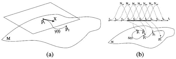
Recent work in [12] on continuous tensor field approximation achieves smoothness; however, a Riemannian framework is not employed for tensor calculations. In this section, we define tensor splines that are curves interpolating or approximating matrix valued functions, constructed using the geometry of the space of SPD tensors. Note that we are defining tensor-splines by doing weighted intrinsic averages on P(n) and choosing the weight functions to be B-splines. As an illustration of interpolation on a 1-D grid of tensors, Fig. 1(b) depicts the idea of using weight functions (B-splines here) to perform weighted average of tensors using the Riemannian metric. This weighted averaging leads to the desired degree spline interpolant (approximant when used in a fitting problem) of the diffusion tensor data.

Fig. 1.

(a) Tangent space of the manifold M of diffusion tensors at point p₁. The tangent vector X points to the direction of geodesic γ(t) between the points p₁ and p₂. (b) A cubic tensor spline S(t), that approximates p_is of a 1-D tensor field. The given points p_i and the points of the tensor spline S(t) are SPD matrices, elements of the Riemannian manifold M. Seven control points c_i and 11 knots t_i are required. The association between basis functions N_i,4(t), knots t_i and given data points p_i is displayed in this figure.

Let us assume that we have a set of N diffusion tensors (p₀, p₁, …, p_N−1) on a one-dimensional grid, and we need to interpolate between them. Linear (first degree) interpolation on the tensor space can be achieved by simply computing points on the geodesies connecting two consecutive diffusion tensors. Higher degree continuous interpolation can be achieved by using a set of control points and a knot vector. A k − 1th degree tensor spline that fits to our data requires N+k − 2 control points (c₀, c₁, … c_{N+k − 3}) that are also tensors and N + 2(k − 1) monotonically increasing knots (t_−k+1,t_−k+2, …, t_{N+k− 2}). A tensor S(t), where t ∈ [t_j, t_j+1), which is a point on a tensor spline, can now be computed by generalizing (1) to the space of tensors. We can compute the value S(t) of the k − 1th degree B-spline of tensors for a particular t value, by calculating a weighted intrinsic average, Σ̃, of the control tensors c_i, where the weights are the basis functions w_i = N_i,k(t), discussed earlier

$$S(t)={\mathrm{\sum }^{\sim }}_{i=0}^n{w}_i{\mathbf{c}}_i.$$ (4)

The intrinsic weighted average (4) of tensors is defined using the Riemannian distance instead of the Euclidean distance, and it is the minimizer of the function

$$\underset{\mu \in P(n)}{min}\rho (\mu )=\underset{\mu \in P(n)}{min}\frac{1}{2}\sum _{i=0}^n{w}_i\text{dist}{(\mathit{\mu },{\mathbf{c}}_{\text{i}})}^2$$ (5)

where dist(·, ·) is the Riemannian geodesic distance. The weighted average can be computed using a gradient descent algorithm that is an extension of the algorithm described in [3] for computing the mean of tensors. The gradient of ρ(μ) is given by

$${\nabla }_{\mu }\rho =-{\sum }_{i=0}^n{w}_i{\text{Log}}_{\mu }({\mathbf{c}}_i).$$ (6)

Thus, the intrinsic weighted average of a set of diffusion tensors can be computed using the following procedure:

C. Tensor Spline Approximation

In order to fit a tensor spline to the diffusion tensor data, we have to approximate the control tensors of such a spline. A tensor spline that fits to our data, minimizes the Riemannian distance of the given tensors from the tensor spline curve

$$E=\frac{1}{2N}\sum _{i=0}^{N-1}\text{dist}{(S(t_i),{\mathbf{p}}_i)}^2.$$ (7)

In (7), the Riemannian metric should be used for the distance calculation, since the tensor space, where the data and control points live, is a curved manifold (convex cone). We need to find a set of control points (c₀, c₁, …, c_{N − 1+k − 2}) that form the spline S(t) which minimizes the energy E. The gradient of E with respect to c_j is then given by

$${\nabla }_{{\mathbf{c}}_j}E=\frac{1}{2N}{\sum }_{i=0}^{N-1}{\nabla }_{S(t_i)}\text{dist}{(S(t_i),{\mathbf{p}}_i)}^2{\nabla }_{{\mathbf{c}}_j}S(t_i).$$ (8)

The gradient of the square distance between S(t_i) and p_i with respect to S(t_i) equals

$${\nabla }_{S(t_i)}\text{dist}{(S(t_i),{\mathbf{p}}_i)}^2=-2{\text{Log}}_{S(t_i)}({\mathbf{p}}_i)$$ (9)

where Log_S(ti)(p_i) is the Riemannian logarithmic map, which is a tangent vector at S(t_i). Since the gradient of the energy [see (8)] is with respect to c_j, we need to express the gradient in (9) by using tangent vectors at point c_j. Taking this into consideration, (9) can be approximated by the formula Λ_cj(p_i, S(t_i)) = Log_cj(p_i) − Log_cj(S(t_i)), so we obtain

$${\nabla }_{S(t_i)}\text{dist}{(S(t_i),{\mathbf{p}}_i)}^2\approx -2{\mathrm{\Lambda }}_{{\mathbf{c}}_j}({\mathbf{p}}_i,S(t_i)).$$ (10)

Furthermore, the gradient of S(t_i) with respect to c_j in (8) is

$${\nabla }_{{\mathbf{c}}_j}S(t_i)=N_{j,k}(t_i).$$ (11)

Using (11) and (10) in (8), we obtain

$${\nabla }_{{\mathbf{c}}_j}E=-\frac{1}{N}{\sum }_{i=0}^{N-1}{\mathrm{\Lambda }}_{{\mathbf{c}}_j}({\mathbf{p}}_i,S(t_i))N_{j,k}(t_i).$$ (12)

Starting with an initial guess of the control tensors, we can update them by using the gradient descent technique. The new values c′_j of control tensors will be

$${{\mathbf{c}}^{\prime }}_j={\text{Exp}}_{{\mathbf{c}}_j}\left(\frac{1}{N}{\sum }_{i=0}^{N-1}{\mathrm{\Lambda }}_{{\mathbf{c}}_j}({\mathbf{p}}_i,S(t_i))N_{j,k}(t_i)\right)$$ (13)

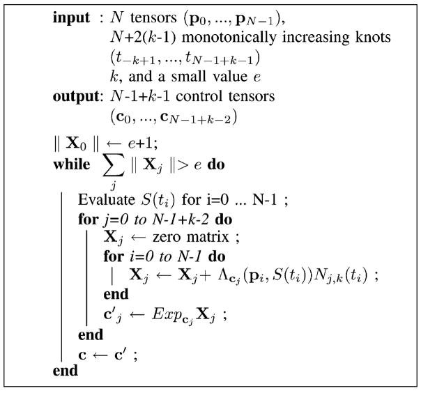
where Exp(.) is the Riemannian exponential map. The initial guess of the control tensors can be either the given data or the average tensor of the given tensors. The gradient descent algorithm is summarized as follows:

The time complexity for a single iteration of Algorithm 2 is of order O((k^dc)N), where k is the degree of the spline, d is the dimensionality of the dataset (for 3-D data d = 3) and c is the number of iterations of Algorithm 2, and N is the given input data size (number of tensors to be approximated). In the experiments that we performed, we found that Algorithm 2 converges in at most in five iterations (c ≤ 5), a CPU time of 9.37 s per iteration on a Pentium 2.4-GHz processor for fitting a cubic (k = 3) tensor spline in a dataset of size 128 × 128. As expected, the time complexity of Algorithm 2 increases as we increase the degree of the spline k or the dimensionality of the dataset d. Note that we chose to provide this machine independent measure of time complexity because execution time will depend on the machine architecture and therefore is not a preferred measure.

Algorithm 2.

Control tensors estimation.

The error introduced by the approximation of (10) can be large, if the tensor spline approximation S(t_i) is far from the target p_i. When S(t_i) tends (moves closer) to p_i during the spline fitting procedure, the error introduced by the approximation of (10) tends toward zero. By setting a small threshold e on the difference between consecutive iterates, the outer loop of Algorithm 2 will be iterated sufficient times in order for the error of (10) to be as small as needed. Thus, the control tensors c_j, which are obtained as the output of Algorithm 2, are estimated by taking the true geometry of P(n) into account.

Tensor splines can be easily extended to higher dimensional tensor fields. For example, consider the case of a 2-D N × M tensor field. A (k − 1)th degree tensor spline that fits to our data requires (N + k − 2) × (M + k − 2) control tensors and (N + 2(k − 1)) × (M + 2(k − 1)) monotonically increasing (in both the dimensions) knots (t_−k+1,_−k+1, …, t_{N+k−+2,M+k−2}). Note that in this case the knots are vectors with two elements, one for each parametric dimension. Finally, the new basis functions are formed by the tensor product of 1-D basis functions N_i,j,k([t₁t₂]) = N_i,k(t₁)N_j,k(t₂).

D. Log-Euclidean Splines

Recently, Arsigny et al. [16] proposed a new log-Euclidean metric for tensor calculations. In this framework, the diffusion tensors are first mapped using the matrix logarithmic map to the space of the symmetric matrices Sym(n). Thereafter, the Euclidean norm is used in all calculations in this space. Finally, by using the matrix exponential mapping, the computed values are mapped back to the manifold P(n). Using the log-Euclidean metric we can also fit a spline to the logarithmically mapped data in the space of symmetric tensors, and after that we can map the interpolated/approximated symmetric tensors back to the space of SPD tensors using the exponential mapping. In Section V, we provide a quantitative comparison between tensor splines and splines using the log-Euclidean metric that we will call “log-Euclidean splines.”

E. Robust Tensor Splines

The presence of outliers is common in DT-MRI data due to noise in the original data obtained from the MR scanners [25]. A robust algorithm should reject these outliers from further consideration in any processing algorithms applied to the dataset.

A robust function can be applied to the energy function, in order to weight the given data p_i appropriately. We can use a robust function that assigns weights in the interval [0, 1], where weights that are almost zero imply rejection of the corresponding data point. Furthermore, high weights should be assigned to the data points whose distance from the unknown spline curve is small and on the other hand lower weights should be assigned to the data points whose distance from the unknown spline is larger. Let us consider the following function φ(x) = e^{−(x2)/(σ2)}, whose derivative ψ(x) has the aforementioned properties. By using the above function φ, the energy function that we want to minimize can be written as

$$E=\frac{1}{2N}{\sum }_{i=0}^{N-1}\phi (\text{dist}(S(t_i),{\mathbf{p}}_i)).$$ (14)

The gradient of this energy with respect to the control tensors now becomes

$$\begin{array}{l}{\nabla }_{{\mathbf{c}}_j}E=-\frac{1}{N}{\sum }_{i=0}^{N-1}\psi (\text{dist}(S(t_i),{\mathbf{p}}_i))\\ \times {\mathrm{\Lambda }}_{{\mathbf{c}}_j}({\mathbf{p}}_i,S(t_i))N_{j,k}(t_i).\end{array}$$

In the above equation the quantity ψ(dist(S(t_i), p_i)), weights the given data points p_i, leading to a spline approximation that is robust to outliers. The distance function dist(.,.), as it was previously mentioned, measures the Riemannian distance between the tensors.

IV. Application to Segmentation of DTI Data

In this section, we pose the DT-MRI segmentation problem in a Bayesian estimation framework, which has many advantages over the deterministic segmentation schemes in that it naturally allows for incorporation of any specific domain knowledge in the form of priors. Moreover, estimates are provided along with the uncertainty in the estimate. Also, one can get a “soft” segmentation, i.e., a probabilistic segmentation when necessary. Our formulation of the segmentation problem is based on recent work on scalar-valued image segmentation work reported by Rivera et al. [26].

We assume that the given DT-MRI dataset p_i consists of K regions, where “i” is the lattice index. Furthermore, we assume that each region is represented by a model S_k(t_i), where k = 1 … K. There are different choices for the model, which can be either piecewise constant or a smoothly varying tensor field model. In the space of diffusion tensors, the piecewise constant model has a parameter θ_k which is a 3 × 3 SPD matrix. Therefore, for this model the equation S_k(t_i) = θ_k holds for all t_i. In the case of smoothly varying tensor fields, we chose a tensor product of tensor splines as our model S_k(t_i), whose parameters are the control tensors c_i defined in Section III-A. The relation between the control tensors and the tensor spline is given by (4).

Let b_ki be the label map, where b_ki = 1 indicates that the diffusion tensor at the ith lattice point belongs to the kth region class and b_ki = 0 otherwise. Considering the above notation, a diffusion tensor dataset can be modeled as being generated using a generative model given by the following equation:

$${\mathbf{p}}_i={\sum }_{k=1}^K{S}_k(t_i)b_{ki}+{\epsilon }_i$$ (15)

where ε_i is assumed to be an independent identically distributed noise process. In this framework, the parameters of the models and the labels b_ki are assumed unknown and must be estimated given a diffusion tensor dataset p_i. The goal then is to estimate these unknowns given the tensor field. A Bayesian framework has been popular in literature for solving such problems and an efficient solution for the scalar field segmentation was previously presented in [26]. Our formulation here extends their formulation to cope with tensor fields.

Let υ_ki be the probability that the diffusion tensor p_i was generated by the kth model. The likelihood of the label field is then given by

$$P_{p\mid b,\mathbf{c}}={\prod }_k{\prod }_i{(v_{ki})}^{b_{ki}}$$ (16)

where c are the control tensors (parameters of the tensor splines). In the case of tensor-valued images, we can define the probability υ_ki as

$$v_{ki}=\frac{1}{\sqrt{2\pi \sigma }}{e}^{-\frac{\text{dist}{({\mathbf{p}}_i,S_k(t_i))}^2}{2{\sigma }^2}}$$ (17)

where dist(.,.) is the Riemannian geodesic distance between two SPD tensors. If we can estimate the marginal probabilities p_ki, the label field for a hard segmentation (assigns labels in a yes/no fashion and not with a probability) can be estimated by the maximum posterior marginals (MPM) estimator [27] which is defined as

$$b_{ki}=\{\begin{array}{ll}1,\hfill & \text{if}{p}_{ki}\ge p_{li},\text{for}k\ne l\hfill \\ 0,\hfill & \text{otherwise}.\hfill \end{array}$$ (18)

By using the above label field estimator, the unknown variables of our problem are the parameters of the models and the marginal probabilities p_ki. There are two ways to estimate the marginals: a) the mean field approximation [28] and b) Gauss markov measure field (GMMF) model [27]. The mean field approximation leads to algorithms that are rather slow and sensitive to noise and the GMMF approach in [27] leads to significantly different (in the sense of entropy) distributions from the true ones. In [26], Rivera et al. developed a clever technique that controls the entropy of the solution distribution and constraints it to be closer to the true distribution. Using the formulation presented in [26], we can efficiently estimate the unknown parameters of the above mentioned GMMF model by minimizing the following energy function:

$$\begin{array}{l}E(p,c)={\sum }_k{\sum }_i({p_{ki}}^2(-\mathit{log}{v}_{ki}-\mu )\\ +\lambda {\sum }_{s\in N_i}{(p_{ki}-p_{ks})}^2)-{\sum }_i{\gamma }_i(1-{\sum }_k{p}_{ki})\end{array}$$

where μ controls the entropy of the marginals, λ controls the smoothness of the label field, and γ_i are Lagrange multipliers that were introduced to enforce the condition ${\sum }_k^K{p}_{ki}=1$.

The purpose of the entropy control is to bias the posterior marginals estimates toward distributions that have low entropy. Also, log υ_ki is introduced instead of υ_ki to make the data term quadratically depend on the model parameters (tensor spline control vertices) c and for the energy function to remain a quadratic positive definite function of the marginal probability υ and μ < 2λ. For a detailed discussion on the nuances of this energy function (for scalar fields that are also applicable here), we refer the reader to [26]. The energy can be minimized using the expectation maximization (EM) procedure or a generalized EM [29].

In this segmentation algorithm, the number of labels K is not a hidden variable and is predefined. This number can be set equal to or greater than the number of regions that a neuroanatomist expects to find in a particular dataset.

V. Experimental Results

This section is divided into two subsections. The first one contains experimental results obtained by testing the approximation of a diffusion tensor field using tensor splines. In the second subsection, the DT-MRI segmentation experiments performed using the proposed algorithm are described.

A. Tensor Spline Approximation Experiments

In this section, we present several tensor spline approximation experiments with noisy synthetic as well as real DT-MRI data. We also present comparisons with four other existing methods to demonstrate the performance of our proposed tensor spline approximation algorithm. We synthesized a tensor field on a 2-D lattice of size 33 × 33. For the generation of this field, a realistic simulation of the diffusion-weighted MR signal using the Söderman-Jönsson equation presented in [30] was performed. Using this process, at each voxel the MR signal was simulated as a function of the angle θ between the applied diffusion gradient and the orientation of the fiber. At each voxel of the 2-D synthetic field, the orientation of the fiber was assumed to be tangent to circles centered at the lower left corner of the field. Using this fiber structure, the diffusion-weighted MR signal attenuation was simulated for 21 orientations that correspond to the second-order tessellation of the icosahedron on a unit hemisphere, using b-value = 1500 s/mm². The diffusion tensor field was estimated from the 21 diffusion-weighted images using a linear least squares technique applied to the log linearized Stejskal–Tanner equation [23]. This diffusion tensor field will be considered as the ground truth field for the experiment described below.

Gaussian noise was added to the real and imaginary parts of the simulated diffusion MR signal and then the magnitude signal computed from this noisy complex-valued data. From this signal, we estimated the diffusion tensors as before and then subsampled it by a factor of 4. This process was repeated for different amounts of signal to noise ratios. The first column of Fig. 2 depicts the primary eigenvector field of the 9 × 9 subsampled noisy tensor fields corresponding to signal to noise ratios of 5.0 (top) and 3.0 (bottom). Our goal now is to compare our tensor spline approximation and interpolation method against existing methods in literature, as well as our own modifications of these techniques.

Fig. 2.

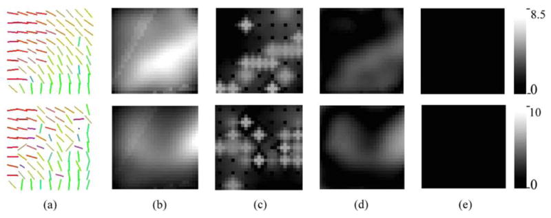
Comparison of approximation methods using a SNR = 5.0 (top) and a SNR = 3.0 (bottom), (a) Primary eigenvectors of the noisy tensor fields. The rest of the columns shows the error in robust approximation using (b) Euclidean spline, (c) PDE interpolation, (d) log-Euclidean spline, and (e) tensor spline. The Riemannian metric was employed for computing these errors.

We first approximated (fitted) the noisy tensor fields by using four different techniques including ours and then interpolated the approximation (fitted) results by a factor of 4. The four methods that we employed were: 1) linear approximation of the elements of the SPD tensors; 2) log-Euclidean geodesic approximation [16]; 3) Riemannian geodesic approximation [3]; and 4) PDE-based anisotropic nonlinear diffusion [17] (Table I). Following this, we present a table of results comparing our method with statistically robust implementation of all the methods (except the PDE-based diffusion filter as its not a simple matter to implement this filter in a robust framework). We also present the results of comparison of a spline version of others’ work with our own, all in a robust framework. In all these comparisons, as expected, our tensor splines algorithms outperformed the competing methods.

Table I.

Approximation Errors in Various Algorithms

	Riem. μ	Riem. σ	Forb. μ	Forb. σ
Euc. Geodesic Appr.	12.2023	10.5576	37.2502	51.8160
Log-Euc Geodesic Appr.	6.5117	7.3565	7.7040	31.4381
Riem. Geodesic Appr.	6.5115	7.3563	7.7037	31.4378
PDE interpolation	8.8490	6.5481	6.3611	29.4992
Non-Robust Tensor Spline	3.8652	2.7202	0.5082	0.8581
Approximation errors using robust function
Robust Euc. Geodesic Appr.	8.6782	0.7521	0.9201	0.1002
Robust Log-Euc Geodesic Appr.	3.8912	2.3191	0.6328	0.928
Robust Riem. Geodesic Appr.	3.4711	2.2534	0.6192	0.795
Robust Tensor Spline Appr.	0.1373	0.0463	0.0015	0.0006
Approximation errors of robust splines using different metrics
Robust Euc. Spline Appr.	7.4655	0.4931	0.0988	0.0927
Robust Log-Euc Spline Appr.	1.4651	0.9996	0.0328	0.0318
Robust Tensor Spline Appr.	0.1373	0.0463	0.0015	0.0006

We use two methods to measure the distance of the estimated tensor fields from the ground truth tensor field: a) the Riemannian metric and b) the Frobenius norm defined as $\sqrt{\text{trace}((\mathbf{A}-\mathbf{B}){(\mathbf{A}-\mathbf{B})}^T)}$, where A and B are two SPD matrices. These errors are computed at each voxel and the mean (μ) and standard deviation (σ) of these errors (denoted by Riem. μ, Forb. μ and Riem. σ, Forb. σ, respectively) are reported in Table I for the noisy dataset corresponding to a signal-to-noise ratio of 3.0. As evident, the error is much smaller for our algorithm in comparison to the others. These results demonstrate the superior performance of our algorithm over other existing methods.

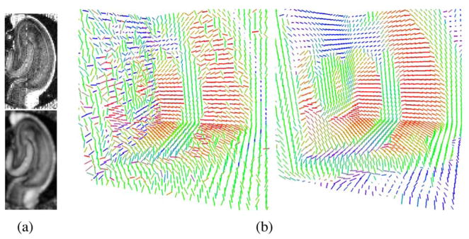
Fig. 3 shows a real data example from an isolated rat hippocampus. The diffusion weighted MR images for this example were acquired using the following protocol. This protocol included acquisition of 22 images using a pulsed gradient spin echo pulse sequence with repetition time (TR) = 1.5 s, echo time (TE) = 28.3 ms, bandwidth = 35 kHz, field-of-view (FOV) = 4.5 × 4.5 mm, matrix = 90 × 90 with 20–30 continuous 200-μm-thick axial slices (oriented transverse to the septotemporal axis of the isolated hippocampus). After the first image set was collected without diffusion weighting (b ~ 0 s/mm²), 21 diffusion-weighted image sets with gradient strength (G) = 415 mT/m, gradient duration (δ) = 2.4 ms, gradient separation (Δ) = 17.8 ms, and diffusion time (T_δ) = 17 ms were collected. Each of these image sets used different diffusion gradients (with approximate b values of 1250 s/mm²) whose orientations were determined from the second-order tessellation of an icosahedron projected onto the surface of a unit hemisphere. The image without diffusion weighting had 36 signal averages (time = 81 min), and each diffusion-weighted image had 12 averages (time = 27 min per diffusion gradient orientation) to give a total imaging time of 10.8 h per hippocampus. Temperature was maintained at 20 ± 0.2°C throughout the experiments using the temperature control unit of the magnet previously calibrated by methanol spectroscopy.

Fig. 3.

Real DTI from an isolated rat hippocampus: (a) FA maps before (top) and after (bottom) tensor spline approximation. (b) principal eigenvector field after log-Euclidean geodesic approximation (left), and nonrobust tensor spline approximation (right).

In Fig. 3, the proposed tensor spline approximation algorithm is compared with the recently proposed log-Euclidean metric based approximation algorithm [16], described earlier. Fig. 3(a) depicts the FA map of the original (noisy) and the approximated data. Note that the FA map after the approximation is much smoother that the FA map prior the approximation (3(a) bottom). Fig. 3(b) shows a 3-D view of the results using log-Euclidean geodesic approximation (left) and nonrobust tensor spline (right) algorithms. Notice that in the tensor spline approximation results the noise has been considerably smoothed out. This may be attributed to the higher order smoothness imposed by the tensor spline developed in this work.

B. DTI Segmentation Experiments

In this section, several segmentation experiments with noisy synthetic tensor fields as well as real diffusion tensor data of an isolated rat hippocampus are presented. Validation results are also presented to demonstrate the performance of our proposed algorithm for diffusion tensor field segmentation under different amounts of noise in the data.

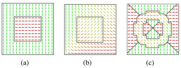
We synthesized several 2-D synthetic tensor fields of size 32 × 32, with different shapes of regions and different anatomy of the diffusion tensor field in each region. All synthetic tensor fields were generated by simulating the diffusion-weighted MR signal [30] as described earlier in Section V-A. Fig. 4(a) and (b) present tensor fields consisting of two piecewise constant regions: 1) a small square region in the center of the tensor field and 2) the region forming the rest of the tensor field. The FA is 0.6 in both regions. In Fig. 4(a), the tensor field within the regions is piecewise constant, while in Fig. 4(b) it is smoothly varying. Finally, Fig. 4(c) consists of the following regions: 1) a ring with principal eigenvectors tangent to circles centered in the lower left corner of the image; 2) two triangular regions with horizontal principal eigenvectors; and 3) two triangular regions with vertical principal eigenvectors. The last two regions have the same FA equal to 0.6, while within the ring the FA is 0.8.

Fig. 4.

Segmentation of various synthetic tensor fields. Figures depict the estimated boundaries between regions and the corresponding primary eigenvector fields.

We segmented the three tensor fields of Fig. 4 using the proposed entropy controlled segmentation algorithm described in Section IV. The parameters of the algorithm that we used are λ = 1 and μ = 0.1. The segmentation results (boundaries between segmented regions) are presented in Fig. 4. The results are as per expectation.

In order to demonstrate the segmentation performance of our proposed algorithm under partial voluming effects, we synthesized a 2-D field consisting of two rectangular regions; the region on the left consists of fibers with orientations parallel to x-axis, and the region on the right is composed of fibers with orientations parallel to y-axis (Fig. 5). Diffusion-weighted images for this 2-D field were obtained by simulating the MR signal, similarly to previous experiments. Then the diffusion-weighted images were averaged using a 10 × 10 kernel, which produces a single average measurement per image for every 10 × 10 pixels. This process was repeated for different locations of the averaging kernel and each time the corresponding tensor field was estimated from the averaged images (see illustration in Fig. 5). The estimated tensor fields were then segmented using our proposed algorithm. The segmentation performance defined as the ratio of the correctly classified area over the total area was computed for the pixels on the boundary between the two regions, and found to be 0.75. For the rest of the pixels (nonboundary pixels) this ratio was 1.0. Finally, we synthesized a 320 × 320 tensor field similar to the one in Fig. 4(c), and then by following the above averaging process we filtered the tensor field down to a) 32 × 32 and b) 64 × 64. After that, the two obtained tensor fields were segmented using our algorithm and the segmentation performance found to be 0.92 and 0.96, respectively. These high values indicate the relative insensitivity of our algorithm to partial voluming.

Fig. 5.

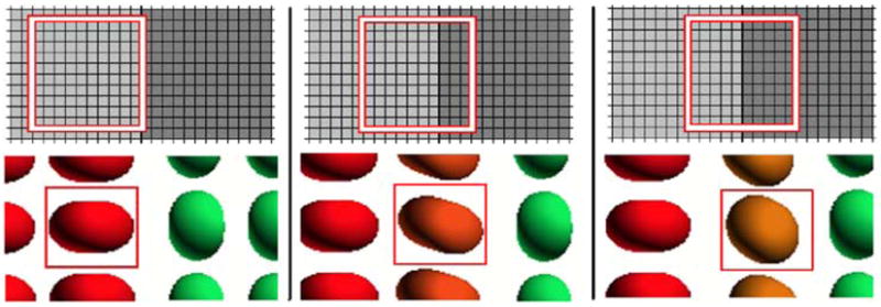
Illustration of segmentation under partial voluming effects. Top: averaging kernels at different locations of the diffusion-weighted images. Bottom: corresponding estimated tensor fields.

In the following experiments, we used the real diffusion tensor dataset from an isolated rat hippocampus, shown earlier in Fig. 3. Fig. 6 presents segmentation results on a 2-D slice selected arbitrarily from the 3-D dataset. Fig. 6(a) depicts the fractional anisotropy (FA) map segmentation obtained using the scalar field entropy-controlled segmentation algorithm presented in [26]. Since the FA map does not contain any information about the orientation of diffusion, as expected, its segmentation yields erroneous results when compared to the expert’s hand segmentation shown as an overlay in Fig. 6(d), taken as the ground truth. This example demonstrates that the tensor field segmentation obtained by segmenting a scalar-valued function computed from the tensors would not suffice in achieving the desired results. Fig. 6(b) depicts the segmentation result using a piecewise constant model in our tensor field segmentation algorithm described earlier and Fig. 6(c) depicts the segmentation result using a piecewise smooth segmentation model. Finally, in Fig. 6(d), we compare our results (shown in the background) with a manually labeled segmentation, based on expert knowledge of hippocampal anatomy (shown as an overlay).

Fig. 6.

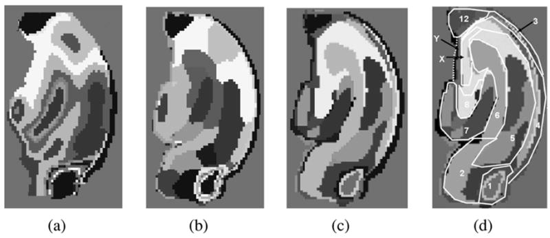
2-D segmentation of an isolated rat hippocampus DT-MRI: (a) FA map segmentation using algorithm in [26] (b) tensor field using piecewise constant models, (c) tensor field using a smoothly varying representation of the regions, and (d) comparison of our results (shown in the background) with a manually labeled image based on knowledge of hippocampal anatomy (shown as an overlay). The index of the labels corresponds to: 1) dorsal hippocampal commissure, 2) subiculum, 3) alveus, 4) stratum oriens, 5) stratum radiatum, 6) stratum lacunosum-moleculare, 7) molecular layer, 8) hilus, X) mixture of CA3 stratum pyramidale and stratum lucidum, Y) stratum oriens but ambiguous, 12) fimbria.

There were some differences between expert manual segmentation and the automatic segmentations of the rat hippocampus, although automatic segmentation based on the smoothly varying tensor spline model better matched the expert manual segmentation than the segmentation based on the piecewise constant model. Expert manual segmentation of the rat hippocampus was based on previous knowledge of hippocampal cytoarchitecture obtained from 2-D visualization of the hippocampus with contrast generated by immunochemistry, various histological staining methods, and tracer studies [11]. The differences appreciated and boundaries denoted by these older techniques offer only indirect or inferential information about the orientations of neurons and glia within the hippocampus. Thus, manual segmentation may differ significantly in certain hippocampal regions from automatic segmentation based on the tensor model of fiber coherences in the rat hippocampus. It must be further considered that study of the hippocampus using these new methods may produce novel insight into the cytoarchitecture of different hippocampal regions not previously known based on previous techniques.

Finally, we present results of segmenting the whole 3-D volume of the isolated rat hippocampus using our segmentation algorithm with the smoothly varying tensor spline representation of the regions. Fig. 7(a) presents a 3-D view of most of the regions detected by the proposed algorithm. Finally, Fig. 7(b) shows different views of the molecular layer contained in the segmentation result shown in Fig. 7(a). To the best of our knowledge, this is the first report on automatic segmentation of an isolated hippocapmus. The clinical significance of an algorithm for automatic segmentation of an isolated hippocapmus has already been discussed earlier.

Fig. 7.

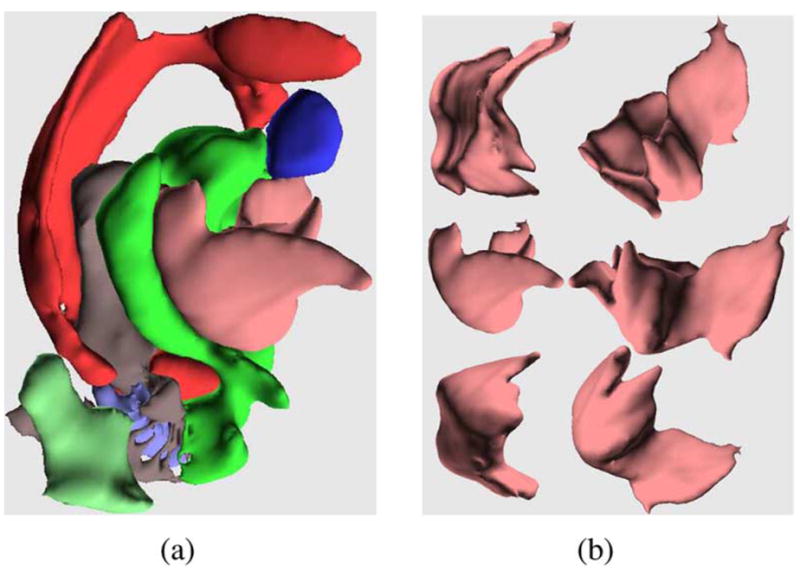
(a) View of the 3-D segmentation of an isolated rat hippocampus, (b) Different views of the molecular layer from the segmentation in (a).

VI. Discussion and Conclusion

Interpolation and approximation are fundamental problems in image analysis and arise in many applications such as DT-MRI registration, DT-MRI segmentation, DT-MRI atlas construction, etc. Scalar-valued and vector-valued image/function interpolation is quite popular in literature. Splines have distinguished themselves as the key ingredient in achieving these goals. To the best of our knowledge, there is no work to date on splines for interpolation and approximation of matrix-valued (second-order tensor valued) datasets using the Riemannian framework. In this paper, we presented a novel and robust spline interpolation and approximation algorithm that we dub tensor-splines, given a noisy symmetric positive definite tensor field. We evaluated the performance of our algorithms on several synthetic and real diffusion tensor field datasets. Our algorithms performed fairly accurately on all the datasets.

For the generation of all the synthetic datasets used in the experimental section, we simulated the diffusion-weighted MR signal using the Söderman-Jönsson equation [30]. The simulation performed by this equation is a simplified version of the process within a real neural tissue, and it can be used for validation of the algorithms proposed in this paper. Another advantage of using this simulation method is that the synthetic noise can be added directly to the diffusion-weighted images, and it has the same characteristics as the noise in real data.

A large amount of the noise that is present in the diffusion tensor datasets (synthetic and real) was removed by approximating the datasets with a robust tensor product of cubic tensor splines using the proposed tensor field approximation algorithm. We implemented this algorithm using different metrics: a) Euclidean, b) log-Euclidean, and c) Riemannian. In all our experiments, the Riemannian metric yielded the best results in approximating a given tensor field. The robust function presented in Section III-E was employed in our experiments, using for each metric the appropriate value for the parameter σ that yields the best results for the metric. The choice of this particular robust function is justified by the fact that it has been commonly used in literature. We have also performed experiments using other robust functions [31] and finding only minor differences in the results of our algorithm. In all our experiments we used cubic (degree = 3) tensor splines since continuity higher than the second order cannot be detected in general by the human eye and this degree of continuity has been commonly used.

An application of our tensor spline algorithm to segmentation of DT-MRI data was also presented. In the context of DT-MRI segmentation, there are a handful of segmentation techniques currently in literature, including work earlier from our own group. Most of these techniques use the level-set framework for segmentation and mostly handle bimodal situations i.e., images containing two classes of regions. In this paper, we presented a novel extension of an efficient GMMF-based Bayesian technique for scalar-valued image segmentation to the tensor valued case using our tensor spline model. DT-MRI segmentation yields much more than what one would obtain with segmentation of contrast-based MRI. It would reasonable to say that the former subsumes the later.

Automated segmentation of DT-MRI from an isolated hippocampus to date has not been reported in literature. Shape and volume changes in different hippocampal regions are thus far the best surrogate markers of hippocampal disease in patients with epilepsy, Alzheimer’s disease, depression, etc. [32], thus making these types of data extremely useful clinically. We presented results of segmentation from an application of our algorithm to an isolated rat hippocampus. We also presented visual comparison of our segmentation results to a hippocampal atlas, showing satisfactory performance of our algorithm. Our future work will be focused on applying our interpolation and approximation algorithms as a module in other applications such as registration of DT-MRI, tractography, etc.

Algorithm 1.

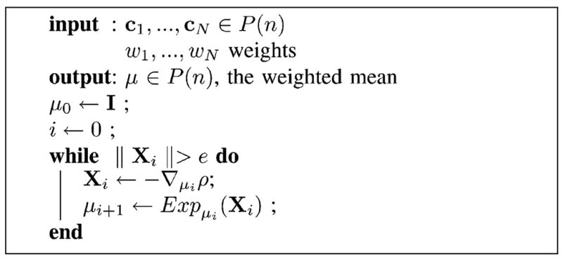
Intrinsic weighted mean of tensors.

References

- 1.Basser P, Mattiello J, Lebihan D. Estimation of the effective self-diffusion tensor from the NMR spin echo. J Magn Reson B. 1994;103:247–254. doi: 10.1006/jmrb.1994.1037. [DOI] [PubMed] [Google Scholar]
- 2.Terras A. Harmonic Analysis on Symmetric Spaces and Applications. II New York: Springer-Verlag; 1988. [Google Scholar]
- 3.Fletcher P, Joshi S. Principal geodesic analysis on symmetric spaces: Statistics of diffusion tensors. Proc CVAMIA. 2004:87–98. [Google Scholar]
- 4.Wang Z, Vemuri BC. An affine invariant tensor dissimilarity measure and its applications to tensor-valued image segmentation. Proc IEEE Comput Soc Int Conf Comput Vision Pattern Recognit. 2004;1:228–233. [Google Scholar]
- 5.Wang Z, Vemuri BC. DTI segmentation using an information theoretic tensor dissimilarity measure. IEEE Trans Med Imag. 2005 Oct;24(10):1267–1277. doi: 10.1109/TMI.2005.854516. [DOI] [PubMed] [Google Scholar]
- 6.Lenglet C, et al. Statistics on multivariate normal distributions: A geometric approach and its application to diffusion tensor MRI. INRIA Res Rep. 2004;5242 [Google Scholar]
- 7.Pennec X, et al. A Riemannian framework for tensor computing. Int J Comput Vis. 2005;65 [Google Scholar]
- 8.San-Jose Estepar R, et al. First International Symposium, ISVC 2005. Vol. 3804. New York: Springer–Verlag; 2005. Riemannian mean curvature flow; pp. 613–620. Lecture Notes in Computer Science. [Google Scholar]
- 9.Amaral D, Witter M. The Rat Nervous System. New York: Academic; 1995. Hippocampal formation; pp. 443–493. [Google Scholar]
- 10.Squire L, Stark C, Clark R. The medial temporal lobe. Annu Rev Neurosci. 2004;27:279–306. doi: 10.1146/annurev.neuro.27.070203.144130. [DOI] [PubMed] [Google Scholar]
- 11.Shepherd TM, et al. Structural insights from high-resolution diffusion tensor imaging and tractography of the isolated rat hippocampus. NeuroImage. 2006;32(4):1499–1509. doi: 10.1016/j.neuroimage.2006.04.210. [DOI] [PubMed] [Google Scholar]
- 12.Pajevic S, et al. A continuous tensor field approximation of discrete DT-MRI data for extracting microstructural and architectural features of tissue. J Magn Reson. 2002;154(1):85–100. doi: 10.1006/jmre.2001.2452. [DOI] [PubMed] [Google Scholar]
- 13.Barr AH, Currin B, Gabriel S, Hughes JF. Smooth interpolation of orientations with angular velocity constraints using quaternions. Proc SIGGRAPH. 1992:313–320. [Google Scholar]
- 14.Batchelor PG, et al. A rigorous framework for diffusion tensor calculus. Magn Reson Med. 2005;53:221–225. doi: 10.1002/mrm.20334. [DOI] [PubMed] [Google Scholar]
- 15.Lenglet C, et al. DTI segmentation by statistical surface evolution. IEEE Trans Med Imag. 2006 Jun;25(6):685–700. doi: 10.1109/tmi.2006.873299. [DOI] [PubMed] [Google Scholar]
- 16.Arsigny V, Fillard P, Pennec X, Ayache N. Proceedings of MICCAI. New York: Springer; 2005. Fast and simple calculus on tensors in the log-Euclidean framework; pp. 259–267. Lecture Notes in Computer Science. [DOI] [PubMed] [Google Scholar]
- 17.Weickert J, Welk M. Tensor field interpolation with PDEs. Preprint 142, Saarland Univ. 2005 [Google Scholar]
- 18.Westin C-F, Martin-Fernandez M, Alberola-Lopez C, Ruiz-Alzola J, Knutsson H. Tensor field regularization using normalized convolution and markov random fields in a bayesian framework. In: Weickert J, Hagen H, editors. Visualization Image Processing of Tensor Fields. New York: Springer-Verlag; 2005. [Google Scholar]
- 19.Alexander DC, Pierpaoli C, Basser PJ, Gee JC. Spatial transformations of diffusion tensor magnetic resonance images. IEEE Trans Med Imag. 2001 Nov;20(11):1131–1139. doi: 10.1109/42.963816. [DOI] [PubMed] [Google Scholar]
- 20.Zhukov L, Museth K, Breen D, BAH, Whitaker R. Level set segmentation and modeling of DT-MRI human brain data. J Electron Imag. 2003;12(1):125–133. [Google Scholar]
- 21.Feddern C, Weickert J, Burgeth B. Level-set methods for tensor-valued images. IEEE Workshop Variational, Geometric Level Set Methods Computer Vision. 2003:65–72. [Google Scholar]
- 22.Helgason S. Differential Geometry, Lie Groups, and Symmetric Spaces. Providence, RI: Amer. Math. Soc.; 2001. [Google Scholar]
- 23.Stejskal EO, Tanner JE. Spin diffusion measurements: Spin echoes in the presence of a time-dependent field gradient. J Chem Phys. 1965;42:288–292. [Google Scholar]
- 24.de Boor C. On calculating with b-splines. J Approx Theory. 1972;6:50–62. [Google Scholar]
- 25.Wang Z, Vemuri B, Chen Y, Mareci T. A constrained variational principle for direct estimation and smoothing of the diffusion tensor field from DWI. Inf Process Med Imag. 2003:660–671. doi: 10.1007/978-3-540-45087-0_55. [DOI] [PubMed] [Google Scholar]
- 26.Rivera M, Ocegueda O, Marroquí JL. Entropy controlled Gauss-Markov random measure field models for early vision. VLSM. 2005:137–148. [Google Scholar]
- 27.Marroquí JL, Velasco FA, Rivera M, Nakamura M. Gauss-Markov measure field models for low-level vision. IEEE Trans Pattern Anal Mach Intell. 2001 Apr;23(4):337–348. [Google Scholar]
- 28.Zhang J. The mean field theory in EM procedure for Markov random fields. IEEE Trans Signal Process. 1992 Oct;40(10):2570–2583. [Google Scholar]
- 29.Neal R, Barry R. Learning in Graphical Models. Dordrecht, The Netherlands: Kluwer; 1998. A vew of the EM algorithm that justifies incremental, sparse, and others variants; pp. 355–368. [Google Scholar]
- 30.Söderman O, Jönsson B. Restricted diffusion in cylindrical geometry. J Magn Reson. 1995;A(117):94–97. [Google Scholar]
- 31.Black MJ, et al. Robust anisotropic diffusion. IEEE Trans Image Process. 1998 Mar;7(3):421–432. doi: 10.1109/83.661192. [DOI] [PubMed] [Google Scholar]
- 32.Insausti R, Amaral D. The Human Nervous System. New York: Elsevier; 2004. Hippocampal formation; pp. 871–914. [Google Scholar]