Transmission Dynamics and Control of Severe Acute Respiratory Syndrome

Abstract

Severe acute respiratory syndrome (SARS) is a recently described illness of humans that has spread widely over the past 6 months. With the use of detailed epidemiologic data from Singapore and epidemic curves from other settings, we estimated the reproductive number for SARS in the absence of interventions and in the presence of control efforts. We estimate that a single infectious case of SARS will infect about three secondary cases in a population that has not yet instituted control measures. Public-health efforts to reduce transmission are expected to have a substantial impact on reducing the size of the epidemic.

SARS is a recently described illness of humans with a high case-fatality rate (1) that has spread widely since November 2002. Probable cases have been reported in 31 countries, with extensive ongoing transmission in Taiwan and China, continuing transmission in Hong Kong, and major outbreaks that are now under control in Singapore (Fig. 1A) and Vietnam (2). The causative agent of SARS appears to be a novel coronavirus (3-5).

Fig. 1.

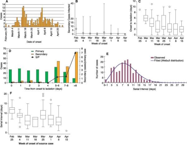
Quantitative epidemiology of SARS as reported from Singapore. (A) Epidemic curve for cases reported up to 5 May 2003. (B) The number of secondary cases infected by an index case reported by week (mean indicated by circles; minimum and maximum indicated by error bars); horizontal line indicates 1, the minimum for epidemic growth. (C) Time from onset of symptoms until hospital isolation of the case, stratified by week of onset. (D) Number of primary cases (green) by time from symptom onset to isolation, number of secondary cases infected by such cases (orange), and mean number of secondary cases per primary case. (E) Serial intervals for known transmissions in Singapore: time from onset of symptoms in index case to onset of symptoms in secondary case with fitted Weibull distribution. (F) Serial intervals stratified by week of onset in the index case. (B), (C), and (F) exclude the final week of data to avoid possible censoring bias. In the box-whisker plots [(C) and (F)], the box extends from the 25th to 75th percentile of observations [interquartile range (IQR)], with the center line indicating the median. The bars define the upper and lower adjacent values, defined as 75th percentile + 1.5 IQR and 25th percentile − 1.5 IQR. The circles denote observed points outside the adjacent values or single observations in a period.

We have used mathematical models of SARS transmission to estimate the infectiousness of SARS from the rate of increase of cases, to assess the likelihood of an outbreak when a case is introduced into a susceptible population, and to draw preliminary conclusions about the impact of control measures.

The basic reproductive number of an infection, R₀, is defined as the expected number of secondary infectious cases generated by an average infectious case in an entirely susceptible population. This quantity determines the potential for an infectious agent to start an outbreak, the extent of transmission in the absence of control measures, and the ability of control measures to reduce spread. R₀ can be expressed as R₀ = kbD, where k is the number of contacts each infectious individual has per unit time, b is the probability of transmission per contact between an infectious case and a susceptible person, and D is the mean duration of infectiousness. In contrast to R₀, the effective reproductive number, R, measures the number of secondary cases generated by an infectious case once an epidemic is underway. In the absence of control measures, R = R₀x, where x is the proportion of the population susceptible. During the course of an epidemic, R declines because of the depletion of susceptibles in the population and the implementation of specific control measures. To stop an outbreak, R must be maintained below 1.

We analyzed data on the first 205 probable cases of SARS reported in Singapore to obtain relevant epidemiologic parameters (6). The number of secondary SARS cases per index case was highly variable (Fig. 1B) in each week but fell from a mean of 7 for index cases with symptom onset in the first week of the Singapore outbreak to a mean of 1.6 in the second week to a mean below 1 in most weeks thereafter (Fig. 1B) (P < .04, Cuzick test for trend). This decline in secondary cases coincided with the application of control measures, including isolation of SARS cases and quarantine of their asymptomatic contacts. Enhanced surveillance of contacts for the development of symptoms resulted in a decline in the time from symptom onset until hospital isolation (Fig. 1C). Because control measures were rapidly applied, there are too few data from Singapore to provide a reliable estimate of R from the period before the institution of control measures.

We therefore used an alternate approach, estimating R from the rate of exponential growth in the number of cases in several other settings and with the use of data from Singapore on the mean serial interval, defined as the time from the onset of symptoms in an index case to the onset of symptoms in a subsequent case infected by the index patient (7). The mean serial interval (8) in Singapore was 8.4 days (SD = 3.8) (Fig. 1E), although, as expected, it was higher for episodes of transmission in which the index case had onset of symptoms in the first 2 weeks of the outbreak before full-scale interventions were in place (Fig. 1F; mean for first 2 weeks was 10.0 days; SD = 2.8 days).

With the use of these estimates, we estimated values of R on the basis of the number of cases that had been reported by a particular time, Y(t), under four assumptions: (i) Y(t) = 1358 cases reported in Hong Kong on 19 April, t = 63 days after the first case on 15 February (2); (ii) Y(t) = 425 cases reported in Hong Kong on 28 March (2), just before the application of specific measures to control SARS; and (iii) Y(t) = 7919 cases reported worldwide as of 20 May, t = 185 days after the first known case on 16 November 2002 (2). To assess the impact of possibly significant underreporting, we repeated the calculation (iv) under the arbitrary assumption that the true number of cases was Y(t) = 15,000 at t = 185 days.

The spread of SARS in a fully susceptible population in the absence of specific control measures is best reflected by assumption (ii), which provides an approximate estimate of R₀ ranging from 2.2 to 3.6 for serial intervals of 8 to 12 days (9). The other data sets, which reflect uncontrolled spread at the onset of local epidemics followed by increasing efforts at control over time, predictably provide lower estimates (Fig. 2). The effect of even substantial underreporting is relatively small because of the logarithmic contribution of the number of cases to the estimate of R. These values of R are considerably lower than those estimated for most other diseases with respiratory transmission, indicating that control measures have the potential to be more effective at blocking epidemic spread. On the other hand, even an infection with an R of 2, if allowed to spread unchecked in a fully susceptible population, is expected to infect a majority of the population (10).

Fig. 2.

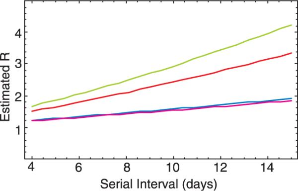
Estimated values of the reproductive number for SARS in the absence of specific control measures for a range of serial intervals from 4 to 15 days (SOM Text). Figure assumes f = 0.3 or 0.7; see fig. S1 for sensitivity analysis for different values of f . Green represents estimated R values for Y(41 days) = 425; red, Y(63 days) = 1358; magenta, Y(185 days) = 7919; and blue, Y(185 days) = 15,000.

The term “superspreading” has been used to describe situations in which a single individual has directly infected a large number of other people; in the Singapore epidemic, of the first 201 probable cases reported, 103 were infected by just five source cases (6). We used the Singapore data and a stochastic transmission model to quantify our uncertainty concerning R attributable to the large variance of the distribution of the number of secondary cases infected by each source case and the uncertainty in that distribution and the serial interval distribution due to sampling variability (11). We found that the credible intervals surrounding our deterministic approximations were wide (Table 1 and Fig. 3). This happens in part because superspreading can have a large influence on the early course of the epidemic. Moreover, the occurrence of index cases that produce large numbers of secondary cases is a rare event whose frequency is impossible to estimate precisely when the epidemic is in its early phases.

Table 1.

90% credible intervals for the value of R from stochastic simulations for four target values. Technical details are given in (11).

	90% credible interval
1358 cases at day 63	(1.4, 4.5)
425 cases at day 41	(1.5, 7.7)
7919 cases at day 185	(1.1, 1.5)
15,000 cases at day 185	(1.1, 1.5)

Fig. 3.

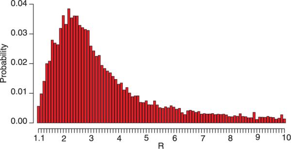
Marginal posterior distribution of R under the Bayesian procedure (11) for Y(41 days) = 425 based on 1000 simulations for each candidate value of R. The most notable feature of the posterior distribution is the considerable right skew, so that although the 90% credible interval spans (1.5, 7.7), the mode is about 2.2 and the expected value is 3.5. Thus, the mode is somewhat lower and the mean somewhat higher than the range obtained by the deterministic approach, which for a serial interval of 8.4 days is 2.2 to 2.6, depending on the value of f used.

If there is large variation in the number of secondary cases generated by each index case, the probability that a single introduction of an infectious case into a population will result in a large epidemic is lessened as compared to the case where the value of R is the same but there is less variation (Fig. 4A). This probability essentially depends on the likelihood that the first case does, indeed, give rise to secondary cases and that several generations of cases take hold before stochastic extinction of the epidemic (12). The probability of an outbreak from a single introduction (Fig. 4A) increases with R, reaching about 80% for R = 2 when the variance in the number of secondary cases is equal to the mean (Poisson distribution). However, if the variance is much larger than the mean, as suggested by the distribution of secondary cases described above, the risk of an outbreak falls significantly. Despite this, the probability of an epidemic increases rapidly when there are multiple introductions (Fig. 4, B to D), Thus, even when the variance is high, epidemic spread is highly likely when R exceeds ∼2 and there are as few as 20 introductions of the infection into a susceptible population. This finding suggests that, if repeated introductions of SARS cases into a population failed to result in ongoing transmission, it would be an indication that control measures have effectively reduced R to levels near, though not necessarily below, 1.

Fig. 4.

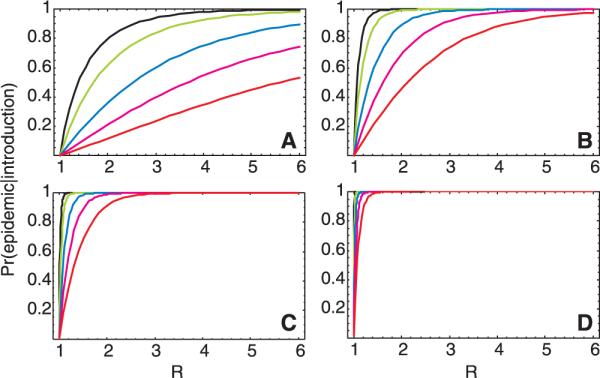
The probability of an outbreak of SARS in a susceptible population for a range of values of R, approximated by the probability of nonextinction of a branching process (22) in which the number of secondary cases is given by a negative binomial distribution with a mean of R and a variance-to-mean ratio ranging from 1 (for which the negative binomial reduces to the Poisson distribution) to 20 [from left to right: 1 (black), 2 (green), 4 (blue), 10 (magenta), 20 (red)] after the introduction of (A) a single infectious case, (B) 5 infectious cases, (C) 20 infectious cases, and (D) 100 infectious cases.

Our approach to estimating R is robust to the possibility that individuals may be asymptomatically infected with SARS and that such individuals may transmit infection. It is currently unknown whether individuals can be infected with SARS but remain asymptomatic and, if so, whether such asymptomatic persons can transmit infection. There is at present no direct evidence of transmission from an asymptomatic person. Indirect evidence that it may occur rarely in normal settings includes a case report of a transmission from an individual whose only symptom was mild fever but who was identified as a SARS case in retrospect (13). Extensive contact tracing in Hong Kong has failed to identify a known symptomatic SARS contact for 8.6% of reported cases (14). We considered the possibility that asymptomatic cases exist and constitute a fixed proportion a of all cases and that these asymptomatic cases transmit at rate kb_a. In this case, the estimated value of R, now given by R = [kb(1 – a) + kb_aa]xD, is unchanged (15). If asymptomatically infected persons become immune to subsequent infection without suffering from SARS, this will ultimately reduce transmission by reducing the susceptible population. However, if asymptomatic persons contribute substantially to transmission but are not readily identified as SARS cases, control measures will be hampered because they depend on the ready identification of people who have been exposed to potentially infectious cases.

Measures to contain SARS have taken two major forms: isolation of symptomatic cases to prevent further transmission and quarantine and close observation of asymptomatic contacts of cases so that they may be isolated as soon as they show possible signs of the disease. To assess the impact of such measures, we constructed a simple, deterministic, compartmental model for SARS transmission, in which a standard susceptible–exposed (noninfectious)–infectious–recovered (SEIR) structure (10) was modified to accommodate quarantine and isolation (Fig. 5). The infection process was modeled in a population (N₀) of 10 million individuals, consistent with the size of a large urban center. We assumed that an infectious individual has a mean of k potentially infectious contacts per day, that susceptible contacts are infected with probability b, and that the number of contacts was independent of population density. We further assumed that individuals are isolated at a fixed rate per day after becoming infectious and that isolated individuals are no longer at risk of transmitting infection. Infected individuals become noninfectious by either dying, recovering, or being isolated, and the mean duration of infectiousness is D days. Quarantine is modeled as follows: Of the bkS/N₀ susceptible contacts infected by an infectious individual each day, a proportion, q, will be sent into quarantine before they themselves become infectious and will remain there until they do become infectious, at which point they are isolated before they can transmit to others; thus, quarantine is assumed to be 100% effective for those contacts who are found before they become infectious. Additionally, a proportion, q, of an infectious individual's daily susceptible contacts who will not go on to develop disease are also quarantined for 10 days, temporarily removing them from the susceptible pool (16, 17).

Fig. 5.

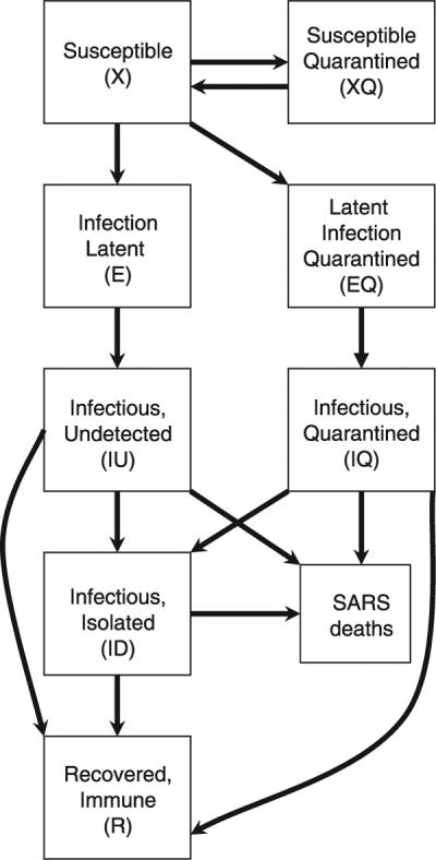
Mathematical model for SARS transmission. Susceptible individuals are infected by infectious, undetected individuals and become infectious themselves after a stage of latency. Infectious individuals lose infectiousness by death, recovery, or isolation. No births or deaths from non-SARS causes are considered. When quarantine is implemented, a proportion, q, of new infections are quarantined before they become infectious; additionally, the same proportion of susceptible individuals who were contacts of infectious persons but were not infected are also quarantined. Susceptible individuals are released from quarantine after 10 days; for simplicity, we assume that quarantined individuals are isolated before they can infect anyone else and that compliance with quarantine is complete (SOM Text).

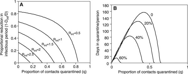
In this basic model, the impact of such control measures is almost completely captured by a simple expression for R in the presence of interventions: R_int = R(1 – q)D_int/D, where D_int is the mean duration of infectiousness in the presence of interventions (Fig. 6A). To reduce R from a value of, for example, 3 to below 1, the combined effect of reducing the infectious period of detected cases and quarantining their contacts (who will then presumably be isolated rapidly once symptomatic) must reduce total infectiousness by at least two-thirds, for example, by a 50% reduction in the infectious period combined with successful quarantine and prevention of transmission by one-third of all contacts. This calculation assumes that individuals are equally infectious throughout the period from the onset of symptoms to isolation. Some early studies of viral titers in nasopharyngeal aspirates suggest that viral shedding increases over the first 10 days after the onset of symptoms (4). If this is reflected as increasing infectiousness with time from onset of symptoms, as hinted by Fig. 1D, then reductions in the mean time to isolation will have disproportionate effects in reducing transmission. In most settings, both interventions will be needed, because both will have limited effectiveness. The effectiveness of quarantine will be compromised by an inability to trace all infected contacts before they become infectious, by any noncompliance with quarantine, and by the possibility that some individuals who comply with quarantine and remain asymptomatic for 10 days will later become symptomatic and infectious. The effectiveness of isolation will be limited by the availability of isolation facilities, by the speed of the isolation process, and by failures of infection control for isolated patients. The importance of health-care settings in the transmission of SARS has been repeatedly documented, and a number of transmission events have occurred even after the index patient had been isolated. Equally important, however, is that from an epidemiologic perspective, prevention of transmission need not be 100% effective, because the reproductive number does not need to be zero to bring the epidemic under control, only reduced and maintained below one.

Fig. 6.

Modeled public-health impact of interventions against SARS including isolation and quarantine. (A) Contour plot showing values of the reproductive number with interventions, R_int, as a function of the proportion of contacts effectively quarantined (q) and the reduction in infectiousness achieved by infection control and isolation. The aim of these interventions is to curtail the epidemic by reducing R_int to less than 1. A baseline value of R = 3 is assumed. (B) The total number of days spent in quarantine per person during the entire course of a SARS epidemic for a given level of effective quarantine. A threshold exists above which quarantining a larger fraction of each infectious case's contacts lowers the number of person-days in quarantine. This threshold is lowered as the duration of infectiousness for each case is reduced by faster isolation, which is indicated by the number next to each curve. Absolute values are for illustration only as they depend on several unknown parameters (SOM Text).

The scale of interventions required to control an epidemic depends on the number of infectious cases present at the time the control measures are instituted and on logistical constraints, such as availability of isolation facilities. Isolation and quarantine procedures will be less effective as more cases accrue (18). Therefore, stringent measures implemented early in the course of the epidemic prevent the need for more stringent measures as the epidemic spreads. Over the course of an epidemic in a closed, homogeneously mixing population, the number of person-days spent in quarantine depends in a complex way on the effectiveness of quarantine and other control measures (Fig. 6B). Above a particular threshold, quarantining a larger fraction of each infectious case's contacts actually results in a lower number of overall person-days in quarantine, because quarantine effectively controls the epidemic so that it more than compensates for the larger number of persons quarantined initially. This threshold and the overall number quarantined are lowered when isolation is used to further reduce transmission. Because the exact threshold value is a function of parameters that are not yet well defined, the model cannot be used to indicate what level of quarantine will be most effective and is meant for illustration only (fig. S2). Figure 6B does, however, suggest that if SARS were allowed to spread over a long period with an R exceeding 1 in a susceptible population, quarantine would impose a large burden on the population, with individuals being quarantined multiple times over the course of the epidemic.

We have used a simple approach based on exponential growth rates in cumulative case numbers to estimate the reproductive number of SARS in the early epidemic in Hong Kong as well as in settings in which initial uncontrolled spread was followed by periods of more effective control. We have further confirmed the robustness of these estimates by using stochastic simulations based on the observed distributions of critical parameters from these settings. These methods capture in simple distributions such complexities as restricted mixing patterns, heterogeneity of transmission in different settings (for example, households and hospitals), and the effects of individual characteristics such as age (1) on transmission and outcomes. Such simplifications allow us to measure the relative impact of a number of specific factors, such as the contributions of superspreading and asymptomatic cases. Future work should certainly focus on quantifying transmission and other epidemiological parameters in a variety of circumstances and use SARS-specific parameters to construct more detailed models of transmission that realistically incorporate the effects of heterogeneities in specific settings. In addition to the control measures considered here, we expect other aspects of SARS transmission, such as the duration of acquired immunity (19), the effect of seasonality on transmission rates (20), and the role, if any, of animal reservoirs, will be important determinants of the future course of the SARS epidemic. These uncertainties make long-term forecasting of the course of the epidemic premature.

The relatively low value we have estimated for R suggests that an achievable combination of control measures, including shortening the time from symptom onset to isolation of patients and effective contact tracing and quarantine of exposed persons, can be effective in containing SARS. Indeed, such measures appear to have formed the basis of effective control in Singapore and Vietnam and have, on a smaller scale, likely contributed to the prevention of major outbreaks in other countries. On the other hand, in the absence of such effective measures, SARS has the potential to spread very widely. Considerable effort will be necessary to implement such measures in those settings where transmission is ongoing, but such efforts will be essential to quell local outbreaks and reduce the risk of further global dissemination.

References and Notes

- 1.Donnelly CA, et al. Lancet. 2003;361 [Google Scholar]
- 2.See information from the World Health Organization (WHO), available online at www.who.int/csr/sarscountry/en/
- 3.Drosten C, et al. N. Eng. J. Med. 2003;348:1967. [Google Scholar]
- 4.Peiris JSM, et al. Lancet. 2003;361:1318. [Google Scholar]
- 5.Ksiazek TG, et al. N. Eng. J. Med. 2003;348:1953. [Google Scholar]
- 6.U.S. Centers for Disease Control and Prevention Morb. Mortal. Wkly. Rep. 2003;52:405. [Google Scholar]
- 7.The reproductive number can be estimated as R = 1 + λv + f(1 – f)(λv)2, where λ = ln[Y(t)]/t is the exponential growth rate of the epidemic, calculated as the logarithm of the cumulative number of cases by time t since the first case divided by the time required to generate these cases from a single case; v is the serial interval; and f is the ratio of the mean latent period, i.e., time from infection to onset of infectiousness, to the serial interval.
- 8.The serial interval is the sum of the mean latent period and the mean duration of infectiousness; neither of these time periods is well defined for SARS. However, there have been no reported cases of transmission of SARS during the presymptomatic period, whereas there is substantial evidence of transmission immediately after onset of symptoms, suggesting that the period of infectiousness begins with the onset of symptoms. The mean incubation period has been variously measured as 5 days (6) and 6.4 days (1), suggesting that reasonable values for f lie in the range of 0.5 to 0.8. Except for the longest serial intervals, estimates of R are relatively insensitive to varying assumptions about f (fig. S1).
- 9.Increasing the assumed serial interval results in a higher estimate of the value of R, because it implies that fewer generations of the infection have occurred in a given time. This range of estimates also includes values obtained for all possible values of f.
- 10.Anderson RM, May RM. Infectious Diseases of Humans: Dynamics and Control. Oxford Univ. Press; Oxford: 1991. [Google Scholar]
- 11.To try to assess the true uncertainty in our knowledge of R, we used a Bayesian approach. We began with a single case at time u = 0. We assumed that a case developing at time u led to a random number, n, of secondary cases at times u + si, i = 1, ..., n. An n was chosen according to a negative binomial distribution with a mean of R and a coefficient of variation (CV) of 3.5, the approximate maximum likelihood estimate (MLE) from the Singapore data. The si values were chosen independently according to a Weibull distribution with shape parameter a and scale parameter b. Let f (Y|R, a, b) denote the density of total number of cases Y by time T and let p(a, b, R) denote the prior. We took p(a, b, R) = p(R) p(a, b), with p(R) uniform on [1.1, 10], p(a, b) as a bivariate normal with a mean equal to the MLE of (a, b), and a covariance matrix equal to the inverse Hessian obtained by the application of Weibull maximum likelihood to the serial interval data from Singapore. Equal-tailed posterior credible intervals in Table 1 were made on the basis of the marginal posterior p(R|Y). The likelihood f (Y|R,a,b) is a complex function of R, a, and b, although draws from the density are easy to simulate. Therefore, to approximate the marginal posterior p(R|Y) ∝f (Y|R) for each value of R in a grid of values in [1.1, 10], we estimated f(Y|R), the integral of f (Y|R, a,b) p(a, b) over a and b, by drawing (aj, bj) from p(a,b), j = 1, ..., J; simulating Yj from f(Y|R, aj, bj), conditioned on fadeout not occurring by time T (i.e., excluding any trial j in which there were no cases in the 20 days preceding T); estimating the density of the Yj with a kernel smoother; and, finally, estimating f (Y|R) as the height of the kernel density estimator at Y. J was at least 200 for all estimates. When the CV of 3.5 was reduced, the credible intervals became smaller (21).
- 12.This can be approximated by the probability of persistence of a branching process (22) in which the number of secondary cases is given by a negative binomial distribution with a mean of R and a given variance. The persistence probability is given as one minus the smallest nonnegative fixed point of the probability-generating function of the branching process (22).
- 13.See information from WHO, available online at www.who.int/csr/sars/archive/2003_05_12/en/
- 14.See information from WHO, available online at www.who.int/csr/don/2003_04_09/en/
- 15.If a proportion a of infectious persons are asymptomatic and differ from symptomatics only in that they have infectiousness ba rather than b, then the fraction of the population ultimately symptomatically infected during the course of an epidemic in an SIR model is simply (1 – a)p, where p is the fraction of the population that is ultimately infected, given implicitly by the equation p = 1 – exp(–R0 p), where R0 is defined analogously to the definition of R in the main text. This is a direct generalization of the usual formula for the final size of an epidemic (10) and is linear because we assume that each case, regardless of its source, has equal probability (1 – a) of being symptomatic. More generally, if these assumptions are met, the ratio of symptomatic to asymptomatic cases will be (1 – a):a (discounting the latent cases).
- 16.If a proportion of infected individuals leave quarantine before they become infectious and are therefore not isolated immediately upon the onset of symptoms, the result is the same as if they had not been quarantined. Our assumption that the proportion of noninfected (still susceptible) contacts of each case who are quarantined will equal the proportion, q, of infected contacts of cases who are successfully quarantined likely represents an underestimate; if contacts are equally easy to trace whether or not they are infected, the proportion of infected contacts quarantined before they become infectious will likely be less than the proportion of susceptible contacts who are quarantined, since some infected contacts will become infectious before they are detected. Since quarantine of infected contacts is more important than quarantine of susceptible ones, we define q in terms of the former.
- 17.In this model, we assume that quarantine of contacts and isolation of cases are completely effective and that those quarantined are at no further risk of infection. These assumptions are made to illustrate the potential impact of control measures. Clearly, special measures will be required to prevent transmission in such situations, especially if large numbers of people are quarantined together.
- 18.Kaplan EH, Craft DL, Wein LM. Proc. Natl. Acad. Sci. U.S.A. 2002;99:10935. doi: 10.1073/pnas.162282799. [DOI] [PMC free article] [PubMed] [Google Scholar]
- 19.Callow KA, Parry HF, Sergeant M, Tyrrell DA. Epidemiol. Infect. 1990;105:435. doi: 10.1017/s0950268800048019. [DOI] [PMC free article] [PubMed] [Google Scholar]
- 20.Dowell SF. Emerg. Infect. Dis. 2002;7:369. doi: 10.3201/eid0703.010301. [DOI] [PMC free article] [PubMed] [Google Scholar]
- 21.Lipsitch M, et al. unpublished data.
- 22.Karlin S, Taylor HM. A First Course in Stochastic Processes. Academic Press; San Diego: 1975. [Google Scholar]
- 23.We thank N. Gay and the WHO SARS modeling working group for their support, S. Lambert of WHO for facilitating our collaboration, B. Bloom for guidance and encouragement in many aspects of this work, K. McIntosh for an introduction to coronaviruses, and R. Malley for helpful comments. Supported by the Ellison Medical Foundation (M.L.) and NIH grants R01 AI 48935 (M.L.), R21 AI 55825 (M.L. and B.C.), T32 AI07433 (T.C.), R01 AI 32475 (J.M.R.), and R01 AI 46669(M.M.). The views expressed in this paper do not necessarily represent those of the City of Hamilton.
Associated Data
This section collects any data citations, data availability statements, or supplementary materials included in this article.