

Abstract
A fast and accurate method to compute the total solvation free energies of proteins as a function of pH is presented. The method makes use of a combination of approaches, some of which have already appeared in the literature; (i) the Poisson equation is solved with an optimized fast adaptive multigrid boundary element (FAMBE) method; (ii) the electrostatic free energies of the ionizable sites are calculated for their neutral and charged states by using a detailed model of atomic charges; (iii) a set of optimal atomic radii is used to define a precise dielectric surface interface; (iv) a multilevel adaptive tessellation of this dielectric surface interface is achieved by using multisized boundary elements; and (v) 1:1 salt effects are included. The equilibrium proton binding/release is calculated with the Tanford–Schellman integral if the proteins contain more than ∼20–25 ionizable groups; for a smaller number of ionizable groups, the ionization partition function is calculated directly. The FAMBE method is tested as a function of pH (FAMBE-pH) with three proteins, namely, bovine pancreatic trypsin inhibitor (BPTI), hen egg white lysozyme (HEWL), and bovine pancreatic ribonuclease A (RNaseA). The results are (a) the FAMBE-pH method reproduces the observed pKa's of the ionizable groups of these proteins within an average absolute value of 0.4 pK units and a maximum error of 1.2 pK units and (b) comparison of the calculated total pH-dependent solvation free energy for BPTI, between the exact calculation of the ionization partition function and the Tanford–Schellman integral method, shows agreement within 1.2 kcal/mol. These results indicate that calculation of total solvation free energies with the FAMBE-pH method can provide an accurate prediction of protein conformational stability at a given fixed pH and, if coupled with molecular mechanics or molecular dynamics methods, can also be used for more realistic studies of protein folding, unfolding, and dynamics, as a function of pH.
Introduction
About 30% of the residues (namely, Asp, Glu, His, Lys, Tyr, and Arg) of proteins are ionizable.1 The ionization equilibria depend on several solution variables such as the pH, salt concentration, temperature, and so forth, as well as on the conformation of the protein. In particular, ionization equilibria are an important determinant of protein structure and function because they define the charges of the ionizable groups and, consequently, the long-range electrostatic interactions that characterize intra- and intermolecular interactions and protein–solvent interactions. A realistic estimation of the stability of a protein in aqueous solution has to take account of both the solvation free energy, as an interaction with the surrounding solvent, and the ionization free energy of the protein at a given pH, that is, as the free energy of the proton binding/release equilibrium. The observed pKa's of the ionizable groups depend on the conformation of the molecule and on the environment of these groups in the macromolecule;2 that is, the folding pathway of a polypeptide in aqueous solution is tightly coupled with its ionization equilibria. Traditional approaches for treating polypeptides and proteins in molecular mechanics and molecular dynamics neglect this interdependency between conformation and ionization equilibrium by simply assuming that the charges on the amino acid residues are invariant to conformational changes. For a given pH, the residues are assumed to be charged or neutral at the beginning of a simulation, and this charge distribution is kept constant throughout the entire simulation.
The reason for such a crude approximation is very simple: there is a large computational price to pay when the more realistic approach is used. The 2ζ possible ionization states of the whole molecule for every conformation have to be considered, with ζ being the number of ionizable groups in the molecule. As a consequence, adoption of a fixed charge distribution during a simulation may introduce an undesired bias to the folding process. Hence, because of its importance in the study of biological processes, the theory of protein titration has been the subject of extensive research for many decades.3–12 Recent evidence12–14 indicates that a correct description of electrostatic interactions that considers all states of ionization may be crucial for understanding protein stability and, consequently, for discriminating the native state from non-native conformations. To alleviate the effort required for the computation of the 2ζ possible ionization states in large molecules, different research groups15–18 have developed approximate solutions to solve the proton binding/release equilibrium problem. Among them, molecular dynamics (MD) with Monte Carlo (MC) sampling of the protonation states has been adopted.15–18 In these applications, the ionization states are selected by using a MC procedure with a Metropolis criterion based on the free-energy difference between protonation states. With the newly selected distribution of charges, a series of MD steps is carried out in an implicit or explicit water solvent. The procedure is repeated iteratively. It is worth noting that MD simulations at fixed pH make use of several other approximations, such as the use of a set of additional continuous coordinates, 0 > λi > 1, to describe the ionization degree of site i, with λi representing the charge state of site i.19–22
There are two major issues that must be addressed before carrying out simulations in which proton binding/release equilibrium is considered. First, the enormous number of ionization states, that is, ∼2[N/3] for a protein with N residues (of which ∼30% are ionizable), should be treated properly,13,14 recognizing that, because its exact treatment is prohibitively expensive, an exact solution to this problem is restricted to proteins with no more than ∼25 residues.14 Any approximation used to surmount such a problem forces us to deal with the accuracy of the computed results.20 A solution to this problem, in the treatment of large proteins, relies on the method adopted to calculate the average ionization degree of each of the ionizable sites, for example, by use of a MC random walk in the ionization space and of the Tanford–Schellman integral method, given by Tanford23 and later by Schellman,24 with an explicit expression by Yang and Honig.25
Second, a fast and accurate method to compute the solvent polarization free energy, for a given fixed protein conformation, is needed. A solution to this problem, representing a further development of the treatment given in refs 10 and 26 will be provided.
A practical implementation of such approaches requires answers to some questions, which are addressed here: (a) what is the optimal algorithm to compute the multisite ionization energy and (b) what is the optimal set of parameters to produce a fast and accurate method? Solutions of these problems, for a given protein conformation at a fixed pH, are provided here by a new algorithm that generalize the fast adaptive multigrid boundary element (FAMBE) method.26 This new algorithm enables one to increase the speed of electrostatic calculations markedly for large proteins without loss of accuracy. It will provide us with both the solvation free energies of the ionizable residues in water and an accurate solution to the free energy of ionization equilibrium, with the use of the Tanford–Schellman23–25 integral. A test on three proteins, which differ in the number of residues, the three-dimensional topology, and the biological function, illustrates the accuracy of the method.
Methods Section
Theoretical Background
The process of dissolving a protein in water in the presence of hydrogen ions can be modeled as a four-stage thermodynamic process:10 (1) creation of a solutesized cavity in water; (2) insertion of the zero-charged protein (with all atoms having zero partial charge) into the cavity in water; (3) charging of the protein to the gas-phase partial atomic charges in which all ionizable groups are maintained neutral; and (4) an equilibrium titration of the protein from pH = ∞ (i.e., zero hydrogen ion concentration) to a given pH value. The first three stages of this partition describe the solvation of a neutral protein. The whole thermodynamic cycle defines the total free energy G(x,pH) of a single protein molecule in water at a given fixed pH in an instantaneous microscopic conformation x
| (1) |
where U0mol(x) is the intramolecular conformational potential energy of the protein computed in a gas-phase approximation, Gcav(x) is the free energy for creation of the molecular cavity in water (stage 1), Gs,vdw(x) is the free energy of van der Waals interactions between the uncharged protein and the water solvent (stage 2),27 G0pol(x) is the free energy of polarization of the water solvent by the protein with gas-phase partial charges on all atoms but with the ionizable groups in the neutral state (stage 3), and the last term ΔG inz(x,pH) is the free energy of ionization of the protein at a given pH with respect to the gas-phase atomic charges as a reference state in which all ionizable groups are neutral (stage 4). The sum of all terms but the first one of eq 1 is equal to the total free energy of protein solvation for a given conformation x at fixed pH.10,27
The only terms of eq 1 that are considered here are G0pol(x) and ΔGinz(x,pH). In addition, since eq 1 pertains to a single conformation x, it is necessary to average over the ensemble of all such conformations.27 However, in interpreting a titration curve, the present practice is to use a single molecular conformation as a representative of the conformational ensemble, although some progress has been made with MC and MD simulations and different electrostatic treatments to treat the whole conformational ensemble.15–22
Multiple-Site Ionization Equilibrium to Compute ΔGinz(x,pH)
To define the ionization free energy ΔGinz(x,pH), we assume that a protein has ζ ionizable groups, and the available 2 ionization microstates are described by the vector z = (1,0,0,1,…,0), where 1 at position i indicates that site i is charged. The underlying theory of multiple proton equilibrium can be found in several previous publications.6–8 The free energy for dissociation of hydrogen ions from an amino acid side chain Si, of the protein P, can be defined relative to the dissociation of hydrogen ions from the isolated amino acid Si by the following scheme
| (2) |
The value of pKa(Si+) of the reference system, that is, of the model compound Si+, is taken from experimental data.5,6 The pKa(1) of a given single ionizable group, indicated by the superscript (1), with all other groups kept neutral, is shifted by ΔpKa(1) due to the protein structure, that is
| (3) |
where the value of pKa(Si+) of the reference system, that is, of the model compound Si+, is taken from experimental data5,6 and the parameter γi is equal to 1 or −1 if the ionizing group is a base or an acid, respectively. Usually, the structure of a model compound Si+ for side chain i is equal to that of the entire residue in the same conformation as it is in the protein PSi+. The free energies in eq 3 consist of two components, namely, the electrostatic intramolecular interactions and the interactions with the solvent. Finally, the free energy of ionization of the single site Si+ in protein P at a given pH, that is, with all other ionizable groups in the protein kept neutral, is given by
| (4) |
The multiple-site free energy of ionization of the protein, ΔGPS+(x,z,pH), from the neutral state z = 0 to the ionization microstate z, is computed as
| (5) |
where GPS(x) is the free energy of the nonionized neutral protein. The energy ΔGPS+(x,z,pH) is a sum of energies of ionization of single sites and pairwise electrostatic interactions between the ionized sites; hence, eq 5 can be rewritten as
| (6) |
where ΔG(PSi+,pH) is given by eq 4 and Δwij(x) is the excess electrostatic potential between ionized sites i,j, with respect to the nonionized sites. By inserting eq 4 into eq 6, the final expression for the free energy of ionization is given by
| (7) |
The ionization free energy of the protein in the conformational microstate x can be calculated exactly from the ionization partition function Zinz as
| (8) |
where the partition function is a sum over all 2ζ ionization microstates z
| (9) |
If the total number of ionizable sites is larger than ∼25, then the number of ionization microstates is greater than 107, and hence, it is prohibitively expensive to evaluate the summation in order to calculate pKa's.10 An alternative accurate and fast approximation to solve this problem for proteins with more than ∼25 ionizable groups follows.
Fast Approximate Method to Calculate pKa's
The ionization free energy, , can be calculated by the thermodynamic integration method as a titration process from zero hydrogen ion concentration to a given value of pH by means of the Tanford–Schellman integral.23–25 From eqs 7–9, the following relations can be obtained:
| (10) |
where 〈ɀi(x,pH)〉 is the average ionization degree of site i, and
| (11) |
From eqs 10 and 11, the Tanford–Schellman integral23–25 can be deduced:
| (12) |
with the functions 〈ɀi(x,pH)〉 and representing the average ionization degree of site Si+ in the protein (PSi+) in conformational microstate x and in the isolated model compound Si+, respectively, and
| (13) |
In eq 13, the free energy term for the sum of all isolated ionizable residues is given by
| (14) |
For site i in protein conformation x at a given pH, the average ionization degrees 〈ɀi(x,pH)〉 can be calculated by a Monte Carlo random walk in the space of the ionization microstates. For pH = ∞, there is only one populated ionization microstate, namely za = (a−,b0), that is, when all acidic residues, za, are negatively charged, a−, while all of the basic residues are neutral, b0. Therefore, a solution for ΔΔGinz(x,∞) can be obtained with eq 6 by computing
| (15) |
For the complementary situation (a0,b+), when all acidic residues are neutral, a0, while all the basic residues are positively charged, b+, an alternative expression for the free energy of ionization can be obtain by integration in eq 12 over the pH interval (−∞,pH) as
| (16) |
while the corresponding ΔΔG inz(x,−∞) value is given by
| (17) |
where the ionization state is zb = (a0,b+).
The ionization free energy can be calculated in two different ways, namely, by integrating from +∞ or from −∞, that is, by using eqs 12 and 15 and 16 and 17, respectively. This offers the opportunity to test the accuracy as well as the internal consistency of the procedure because both ways of integration should give the same results.
Finally, the value of the pKa(PSi+) of ionizable site Si+ in protein P with multiple-site ionization is defined from a titration curve of eq 11 as the value of the pH, that is, pH1/2, at which
| (18) |
In order to compute 〈ɀi(x,pH1/2)〉, it is necessary to compute ΔGPS+(x,z,pH) of eq 7.
Computation of 〈ɀi(x,pH1/2)〉
Continuum Dielectric Model
For a protein embedded in a polar (water) solvent, it is common practice8–10,26,28 to use a continuum dielectric model (Figure 1) to calculate the electrostatic potential φ(r) and the solvent reaction field by solving the Poisson equation
Figure 1.
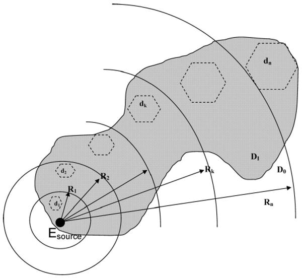
Tessellation of the dielectric interface surface by multisized boundary elements di, with i = 1, 2,…, n, used in the FAMBE-pH method. The large black-filled dot indicates the source Esource. The distances, Ri, from the charged group are shown. Values of di and Ri are reported in Table 4. The shaded region represents the dielectric interface surface of a protein surrounded by water; DI and D0 are the dielectric constants inside and outside of the surface, respectively.
| (19) |
where the charges are qi at position ri in the protein conformation x, with r being the Cartesian coordinates at given positions, ∇ is the gradient, and the dielectric function D(r) is modeled as a sharp dielectric interface, that is, as the surface S(t) of the protein molecular cavity created, in stage 1, by excluding water. The internal volume of this excluded solvent cavity has a low dielectric constant DI, while the solvent has the bulk water dielectric constant D0. The position of the dielectric boundary separating the solute protein from the solvent is chosen empirically in the dielectric model and is defined by the set of atomic radii RDi which are used for calculating the smooth dielectric interface surface.29 The method used to compute the dielectric interface must be defined with precision because it is a crucial component for an accurate prediction in macromolecular applications.27,29–31 For this reason, we use the smooth invariant molecular surface (SIMS) method29 in this work for calculating the dielectric interface surface, that is, the surface of the cavity consisting of the solvent-excluded volume of the protein molecule and an optimized set of Born atomic radii for an accurate modeling of the solvent polarization energy of the protein in water. The SIMS method constitutes an improved algorithm over that of the Richards–Connolly method for calculating molecular surfaces (MS); it smooths all singularities of the Richards–Connolly MS by rolling a probe sphere inside of the MS in order to detect and remove discontinuities in the vector normal to the MS at each point, aimed at producing a uniform distribution of equal-sized surface elements.29
Fast Adaptive Multigrid Boundary Element Method for Solution of the Poisson Equation
The Poisson equation (eq 19) can be converted into an integral equation26 for the induced charge density ζ(t) on the dielectric surface S(t), where t is a surface point
| (20) |
where f = (1/2π)(DI − D0)/(DI + D0), Ei(t) is the electrostatic field [Σk qi,k(t − ri,k)/|t − ri,k|3, where k runs over all charges belonging to ionizable groups i] generated by the set of charges belonging to the charged group i (i = 1,…, Ng; where Ng is the total number of charged groups)26 of the solute, and n(t) is the vector normal to the molecular surface at point t. The induced charge density ζ(t) approximates the average solvent-induced charge density. Since the term Ei(t) is linear in the charges qi, it is possible to split ζ(t) given by eq 20 into a sum of terms, each one of which represents the polarization charge density, ζi(t), generated by a single group of charges of ionizable group i.26 Hence, eq 20 for ζ(t) can be decomposed into a set of independent minor integral equations, one for each of the polarization charge densities, ζi(t)26,27
| (21) |
The reason for such a representation is that the integral in eq 21 for each component ζi(t) can be converted into a discrete linear equation of low dimensionality of a matrix Mi. By this representation over only the set i of adaptive multisized boundary elements,26 we obtain
| (22) |
as an analogue of eq 9 of ref 26. For each charge group, i, the size of the boundary element increases steadily with the distance from the source of the molecular electrostatic field of that charged group, as shown in Figure 1. Hence, for any charge group i, the number of multisized boundary elements, that is, the dimensions of the vectors σi and Ei and the matrix Mi in eq 22, is significantly lower (see Result and Discussion section) than the total number of surface elements that would be encountered if the surface was tessellated by the finest uniform boundary elements of surface area s in eq 21. The number of multilevel boundary elements NMBE which tessellate a MS with area AS scales as
| (23) |
where nloc and Aloc are the average number of boundary elements and the size of the local area with the finest tessellation, respectively, if within R1.
The present adaptive tessellation algorithm is a generalization of the tessellation method by the boundary elements of three size levels, that is, small, large, and surface patches described in ref 26 (a surface patch represents the whole surface of one surface atom). The current tessellation method considers a generalized set of mutually inserted surface boundary elements (BE), that is, surface grids, of different average sizes, with average BE dimensions of di, i = 1, 2, 3,…, n, where i is the level of the BE and n is the total number of levels. The BEs of level i are a set of surface elements with areas and coordinate of center , so that the whole molecular surface can be completely covered by the BEs of each level. Each BE has an average value of polarization charge density which is assumed to be constant over this BE. The BEs of the first, finest level i = 1 are calculated as a set of surface elements by the SIMS29 method with high dot density and small average dimension d1; the BEs of the second level are also calculated by the SIMS29 method with low dot density, with average dimension d2. Each BE of the third level represents the whole surface of one surface atom. Each BE of levels 4, 5, and so forth represent a united surface of a group of nearest atoms. Each BE of level i is a collection of integer numbers of BEs of the previous level i − 1. The surface area, average polarization charge density, and position of the BE of level i are defined as the average values over the respective set of BEs of level i − 1 and are inserted into the BE of level i. That is why the total number of variables in eq 22 is small.
The FAMBE method constructs the adaptive tessellation, which depends on a specific center on the protein surface, for each σi (as given by eq 22). The FAMBE method uses a set of distances Ri for level i (Figure 1), using the boundary element set of level i to tessellate the molecular surface (MS) in the vicinity of point t if the distance rit from the charged group qi to the point t of the MS is in the range of Ri−1 > rit > Ri (the region between two arcs in Figure 1). The dimensions di of the multisized BEs and Ri determine both the accuracy of the numerical solution and the CPU time. The important primary parameters are the size of the finest BEs, d1, and the surface area covered by d1 and defined by R1. All other parameters di and Ri are defined from d1 and R1 recursively by the relations di/di−1 and Ri/Ri−1 described below. An analysis of the dependence of the accuracy and CPU time on the tessellation parameters d1 and R1 for the three-level version of the FAMBE method has been carried out in ref 26. The optimization of the primary parameters of the method for determining d1 and R1 was carried out by Vorobjev and Scheraga26 by comparing the numerical solution of eq 22 with an analytical one for a sphere with a single charge off center. The optimal values obtained for d1 and R1 were ∼0.5 and ∼5.0 Å, respectively. These optimal values of the parameters d1 and R1 are independent of the total number of multisized levels n. Each boundary element (BE) of level i consists of an integer number of boundary elements of the previous level i − 1, in the range of 3–6, with an average value of ∼4; therefore, the average ratio for sizes di/di−1 is ∼2, based on the square root of the ratio of the areas of BE i and i − 1. The relation Ri/Ri−1 ∼ 2 – 1.5 follows from the ratio di/di−1 ∼ 2 and from the required numerical accuracy of the solution of eq 22.
In summary, the use of the SIMS29 method to compute the molecular surface area and the whole tessellation procedure described above are improvements of the corresponding methods used in previous work.26
Each linear equation for σi, as given by eq 22, can be solved iteratively by the preconditioned biconjugated gradient method26 after a few iterations, namely, 4–6. Therefore, the total numerical complexity of the FAMBE method scales linearly with the size of the protein, that is, the number of such equations is linear in protein size, which grows linearly with the number of ionizable groups.
Calculation of the Ionization Equilibrium
The key advantage of the FAMBE method over other solutions of the Poisson equation7–9 is that this method calculates the full set of minor charge densities σi(t) simultaneously, that is, the system of Ng independent equations, given by eq 21 for σi(t), can be solved simultaneously in Ng processors. These quantities are needed for calculating individual polarization free energies of the ionizable groups as well as for computing the electrostatic potential of the mean force Δwij between ionized groups i and j, in eq 7.10,26
The partial charges on all atoms of an ionizable group differ depending on whether the group is charged or neutral, that is, qi+ and qi0, respectively, as in the model compounds Si+ and Si. The set of charges of the whole structure, PSi+, can be represented by qi+ plus the set of all of the other charges QiP of the protein; likewise the total charge of PSi is qi0 plus QiP. Each set of atomic charges induces a corresponding set of solvent polarization charges, namely, σi+, σiP, and σi0, on the boundary elements of the MS, of the molecule (PSi+ or PS, respectively). The set of charges in microstate z can be represented by the set of qz+ charges containing the atomic charges of all ionized groups in the ionization microstate z, while the rest of all of the atomic charges of the protein, except the atoms that belong to the ionized groups z, are represented by QzP. For the neutral state of the molecule, the set of charges in microstate z is represented by the set of qz0 charges, while the rest of all of the atomic charges of the protein, except the atoms that belong to the groups z, are represented by the same QzP. The set of atomic charges qz+, QzP, qz0 induces a corresponding set of solvent polarization charges, namely, σz+, σzP, σz0, on MS (PSz+ or PS, respectively). Using this definition of charges, the total electrostatic free energy of the protein can be represented as a sum of charge–charge interactions between any pair of sets of atomic charges plus the interactions between the charges and the surface-induced charges. After using the reciprocal relation for the product between potential and charge,32 the product of a set of atomic charges with a set of induced charges over the corresponding MS can be described by the following equation
| (24) |
where
| (25) |
is the product between the set qi+ and the set of induced charges σiP on the MS of the structure PSi+, and the subindex α runs over all atoms of the ionizable group i. With these equations, the excess free energy ΔGPS+(x,z,pH) of eqs 5 and 6 can be written as
| (26) |
where an example of the charge–charge product is
| (27) |
where the index η runs over all ionizable atomic charges in the ionization microstate z and Pβ runs over all of the remaining atomic charges of the protein. A similar expression pertains to the other terms of eq 26. It should be noted that the terms in eq can be rearranged into the first sum of eq 6 and the sum of the pair interactions between ionizable sites, that is, the last term of eq 6. With the aid of eq 3, the value of pKa(1)(PSi+) for the ionizable group in eq 7 can be reduced exactly to the following expression
| (28) |
where ΔpKi(1) is the shift in the pKa of the ionizable group Si+ due to the protein environment while all other ionizable groups are neutral, and
| (29) |
| (30) |
| (31) |
The term ΔgP+ is the desolvation penalty for ionization of residue Si+ in the protein environment, relative to the model compound, and is given by the first two terms of eq 29. On the other hand, the last two terms of eq 29 describe the effect of the protein field on the ionizable residue Si+. Similarly, the terms of eq 30 describe the desolvation penalty and the protein field effect for the neutral residue Si. The two terms in eq 31 represent the difference in polarization free energy because of the change in the MS due to protonation of the ith group and have been found to be negligible (see Results and Discussion section).
Rearranging expression 26 as a sum of pair terms gives the excess potential of mean force Δwij(x), shown in eq 6, as
| (32) |
Where
| (33) |
It should be noted that the potential w++ consists of a sum of two terms, representing the direct charge–charge Coulomb interaction, plus representing the solvent reaction field effect, as given by the interaction with the polarization charge density on the protein surface. The term w+0 represents a correction to the interaction between ionized group i and group j due to atomic charges in the neutral state8 and is given by
| (34) |
The 1:1 Salt Effect in the FAMBE Method
The FAMBE method solves the Poisson equation by considering the solvent polarization under zero salt conditions. A rigorous generalization of the boundary element method to an electrolyte solutions is considered in a number of papers.33,34 The main results of such a generalization can be summarized as follows: (i) the conversion of the linear Poisson–Boltzmann equation into the boundary element method gives rise to two coupled integral equations and becomes considerably more complicated than that given by eq 21; (ii) at physiological concentrations of a 1:1 salt, that is, ∼0.1–0.2 M, the free-energy contribution to the total free energy due to the mobile salt ions is small, about 1–2% of the value of the polarization energy of the water solvent in the linear Poisson–Boltzmann method;33,34 and (iii) the major salt effect on the pair of electrostatic interactions is the Debye–Hückel screening of the electrostatic interactions between charged sites.35,36
The 1:1 salt effect is included, indirectly, in the FAMBE-pH method, as was done for the salt-dependent generalized Born method.22 The correction consists of two terms; the first one is a correction of the free energy due to interactions of the ionizable group i with the mobile salt ions and is given by
| (35) |
where the Debye screening constant (inverse length) is given by κD = 8πI/D0kT, with I being the ionic strength, k the Boltzmann constant, T the temperature in K, and D0 the bulk dielectric constant; RQi is the effective radius of the charged group i due to the protein structure and includes the radius of the Stern layer, as explained below in eq 37. The radius RQi is defined in the framework of the generalized Born (GB) method37–39 by calculation of the solvent polarization free energy of the ionized group as
| (36) |
where Gpol,i(x) is the solvent polarization free energy of the ionizable group i, for the protein in conformation x, in the FAMBE method. The effective Born radius, RBi, should be increased by the radius of the hydrated salt ion Rion as
| (37) |
where the value of Rion represents the Stern radius (∼2 Å).28 The contribution of the salt ions to the pK shift is given by
| (38) |
This term should be added to ΔpKi(1) of eq 28. This contribution is usually low (∼0.01 pK unit) because of the small magnitude of the free energy and the mutual cancelation of two terms in eq 38, that is, one of them corresponding to the energy for the isolated site Si+ and the other one as the energy corresponding to this site in the protein, PSi+. Another contribution from the 1:1 salt correction is related to the electrostatic potential of mean force, Δwij, between two ionized sites i and j, which is known35 to be modified by the Debye–Hückel screening factor as
| (39) |
where b = RQi + RQi is an effective distance of minimal approach. This correction is valid for the linear regime of screening, when the Poisson–Boltzmann equation can be linearized under the assumption that the magnitude of the electrostatic potential at the ion-accessible surface of the ionized protein in water is about kT.35,36 At physiological pH, most proteins are in the vicinity of their isoelectric pH with a total charge of only a few units, and hence, they are expected to have a moderate electrostatic surface potential. At low or large values of pH, compared to the isoelectric pH, proteins can have large positive or negative total charge and possess a large electrostatic surface potential, that is, significantly greater than kT. Under these extreme pH conditions, an accurate treatment of the protein electrostatic energy is challenged since the Poisson–Boltzmann equation for mobile ions is no longer valid because it does not take into account the ion–ion correlations. Some discussion of this problem is given in ref 40, but analysis of these limits deserves more research and is beyond the goal of the current work.
Effective Dielectric Constant for the Protein
To compare computed pH-dependent effects of a protein with experimental data, the thermal fluctuations and the response of the protein–solvent system to the protein ionization must be taken into account, that is, the protein dynamics cannot be ignored. Thus, the dynamic response of the polar groups to the ionization of one of the groups in the sequence can be treated, equivalently, as the polarization response of a polar solvent to the charging of a solute atom.41 In this respect, and in the context of the dielectric continuum model, the protein polarization response can be modeled by assigning an appropriate dielectric constant. For example, according to explicit simulation of the dielectric properties of a protein–water system, proper consideration of the polarization response can be obtained by assigning a dielectric constant of DI ∼ 15 and D0 ∼ 50–100 for the protein and water surrounding the protein, respectively.41 For this reason, in the FAMBE method, the pH-dependent properties are computed for a given fixed conformation x, although the protein dynamic polarization response is taken into account implicitly by assigning a dielectric constant of DI = 16 to the volume occupied by the protein and D0 = 80 for the solvent-excluded volume outside of the protein.
Results and Discussion
Optimal Set of Dielectric Interface Atomic Radii RBi
The optimal set of atomic radii RBi for calculating the dielectric surface was determined by fitting the polarization free energy of the FAMBE method, as given by eq 35 of ref 26, to the “experimental” polarization free energies obtained for a set of terminally blocked amino acid residues.42 The “experimental” polarization free energies were simulated by a slow charging process30,43,44 with the molecular dynamics program SigmaX,45 in explicit SPC water,46 with periodic boundary conditions, and with the particle-mesh Ewald (PME)47 approximation to treat long-range electrostatic interactions. On the basis of the hypothesis that the optimal radius RBi should be independent of both the charge distribution and the molecular conformation, the calculation of the solvent polarization free energy shown in Table 1 was carried out for each listed amino acid residue X in the sequence Ac-X-NMe in an extended conformation with the charges taken from the SigmaX45 force-field. Fifteen out of the 30 groups in Table 1 were taken as the training (fitting) set for the calculation of the atomic radii RBi to be used by the FAMBE method. During the fitting procedure, the dielectric constant of the solute cavity, defined by the FAMBE method, was set equal to DI = 1.0, to be consistent with the dielectric constant for a fixed protein conformation in a molecular dynamics simulation of the charging process in explicit water solvent, while the value of the solvent dielectric constant was set to D0 = 80.0. The calculated atomic radii RBi are listed in Table 2, together with the radii obtained by the PARSE48 method shown for comparison. The overall error of the FAMBE method (compared to the slow-charging method) in reproducing the polarization free energies of terminally blocked amino acids (given in Table 1) is equal to 1.6% for the training set (indicated by asterisks in Table 1) and about 2% for the set of 13 groups in Table 1 not included in the fitting procedure.
TABLE 1. Solvent Polarization Free Energy (kcal/mol)a.
| groupb | X | slow-charging method | FAMBE method |
|---|---|---|---|
| AcCO | ALA | −2.98 | −2.93 |
| pepc CO | ALA | −2.96 | −2.95 |
| AcCO-pepc CO* | ALA | −5.40 | −5.66 |
| pepc NH | ALA | −1.73 | −1.74 |
| NMeNH | ALA | −1.89 | −1.94 |
| H2Od | −8.50 | −8.46 | |
| AcALANMe* | ALA | −10.7 | −10.30 |
| pepc NHCO* | ALA | −3.65 | −3.74 |
| pepc NHCO* | GLY | −3.83 | −3.90 |
| pepc NHCO* | VAL | −3.50 | −3.58 |
| pepc NHCO* | LEU | −3.74 | −3.73 |
| sidee COH | SER | −8.20 | −8.22 |
| sidee COH* | THR | −7.31 | −7.15 |
| pepc CONH-sidee CHOH* | THR | −11.30 | −11.58 |
| pepc CONH-sidee CHOH* | SER | −11.60 | −12.04 |
| sidee ASP | ASP | −88.4 | −88.3 |
| sidee GLU−* | GLU | −96.1 | −96.9 |
| sidee LYS+ | LYS | −90.5 | −90.6 |
| sidee ARG+ | ARG | −62.1 | −63.4 |
| sidee HIS0 | HIS | −10.8 | −10.8 |
| sidee NH2 | GLN | −6.35 | −6.22 |
| sidee GLN* | GLN | −8.95 | −8.59 |
| AcGLNNMe* | GLN | −16.1 | −16.1 |
| pepc CONH-sideb | GLN | −10.8 | −10.8 |
| AcASNNMe* | ASN | −21.1 | −20.6 |
| sidee ASN | ASN | −8.90 | −9.03 |
| sidee(NH2)* | ASN | −5.2 | −5.23 |
| pepc-sidee ASN* | ASN | −13.7 | −13.45 |
| sidee PHE | PHE | −0.24 | −0.32 |
| sidee TYR | TYR | −5.75 | −5.63 |
Computed for the charged groups in the terminally blocked amino acid X in Ac-X-NMe by slow-charging simulations31 and also by using the dielectric model (FAMBE) method as described in the Results and Discussion section in the subsection entitled “Optimal Set of Dielectric Interface Atomic Radii RBi”. Asterisks denote the groups used for fitting; “pep” indicates backbone groups, and “side” indicates side-chain groups.
Atomic group undergoing the slow-charging process. The rest of the atoms of the terminally blocked amino acids have zero partial charges. This set covers all polar and ionizable groups in proteins.
Peptide main chain, for example, pepCO is the CO group, and pepNHCO is NH and CO of the peptide main chain, and so forth.
Internal water molecule in proteins.
Group of atoms from the side-chain X.
TABLE 2. Optimal Set of Atomic Radii (RBi)a.
| atom type | (RBi)b (Å) | (RBi)c (Å) |
|---|---|---|
| CH, CH2, CH3 aliphatic (united-atom) | 2.21 | 2.0 |
| CH, C aromatic | 1.72 | 1.70 |
| N | 1.50 | 1.50 |
| N (NH3+) | 1.70 | 2.00 |
| O= | 1.53 | 1.40 |
| O− (COO−) | 1.30 | 1.58 |
| –O– water (SPC) | 1.73 | |
| –O– TYR | 1.65 | |
| –O– SER, THR | 1.45 | |
| H–polar atomd | 1.10 | 1.0 |
| H–O SER, THR | 0.85 | |
| H (NH3+) | 0.87 |
Computed as described in subsection “Optimal Set of Dielectric Interface Atomic Radii RBi.”
Computed in this work.
PARSE set of radii.48
Any H atom bonded to an electronegative donor other than SER and THR, for example, N–H2, N–H, O–H, and so forth.
Internal Self-Consistency Test of the FAMBE Method
The asymptotical form for the total electrostatic potential φ(r) at a large distance from a protein is equal to the sum of the classical multipole terms due to the protein charges qi at the points ri scaled by a factor 1/D0. This condition imposes limits on the multipole moments of induced charge density distribution σ(t) over the dielectric interface surface. Thus, a test (called a Q test) for computing the total charge requires that Qσ ≡ Qq, defined in eq 40
| (40) |
In the FAMBE method, σ(t) satisfies the Q test exactly26 by using a sum rule normalization and smoothing of the matrix elements of Mi of eq 22 to increase the accuracy and numerical stability of the solution. Moreover, the surface-induced dipole moment Mσ should be proportional to the dipole moment of the protein for the set of atomic charges. Then, the M test requires that Mζ ≡ Mq, defined in eq 41
| (41) |
By contrast with eq 40, eq 41 depends on the numerical accuracy of the method. Table 3 shows the results for the self-consistency test for the calculations of the total charge Q and the induced dipole moments M for a set of five proteins. It can be seen from Table 3 that the FAMBE method exactly satisfies the Q test given by eq 40. Moreover, the average error for the M test, given by eq 41, namely, the average ratio |(Mq − Mσ)|/|Mq| (given in the last column of Table 3), does not exceed 2% for the optimal parameters given in Table 4, which provides a compromise between speed, scalability, and accuracy of the solution.
TABLE 3. Total Charge and Induced Dipole Moment on the Dielectric Surface Interfacea.
| protein | Qσb (e.u.) | Qσc (e.u.) | Mσb (Å e.u) | Mqc (Å e.u) | |(ΔM|/|M| | ||||
|---|---|---|---|---|---|---|---|---|---|
| 4PTId | −0.4875 | −0.4875 | −12.982 | −13.432 | 1.290 | −12.887 | −13.361 | 1.279 | 0.005 |
| −0.9750 | −0.9750 | −7.883 | −9.350 | −29.321 | −7.706 | −9.416 | −29.120 | 0.007 | |
| 0.0000 | 0.0000 | 0.851 | −0.357 | −1.641 | 0.814 | −0.430 | −1.618 | 0.035 | |
| 2LZTe | −0.3000 | −0.3000 | −0.083 | −4.517 | −4.296 | −0.103 | −4.682 | −4.512 | 0.038 |
| 0.2375 | 0.2375 | 5.225 | 4.607 | 1.746 | 5.158 | 4.630 | 1.691 | 0.011 | |
| −0.2375 | −0.2375 | 0.373 | −3.556 | −2.845 | 0.321 | −3.571 | −2.842 | 0.012 | |
| 3RN3f | −0.4750 | −0.4750 | −2.744 | 10.053 | 1.017 | −2.603 | 9.699 | 0.650 | 0.035 |
| −0.2375 | −0.2375 | −6.161 | −2.048 | −0.385 | −6.166 | −2.051 | −0.379 | 0.004 | |
| 0.2375 | 0.2375 | 7.489 | 5.457 | 5.614 | 7.502 | 5.510 | 5.742 | 0.008 | |
| 1UBQg | 0.000 | 0.000 | −15.317 | 0.895 | −1.219 | −15.545 | 0.966 | −1.276 | 0.019 |
| 1EA1h | 17.7750 | 17.7750 | −82.532 | −68.768 | 1144.115 | −76.276 | −67.969 | 1147.880 | 0.008 |
Computed by the FAMBE method for different charged states (chosen arbitrarily) of proteins, indicated by each horizontal line for the proteins listed in column 1 by their Protein Data Bank code.
Qσ and Mσ are the induced total charges and dipole moment components computed with eqs 40 and 41, respectively. The three columns under Mσ represent components of the dipole moment Mσ.
Qq and Mq are the total molecular charges and the molecular dipole moment components, computed with eqs 40 and 41, respectively, while |ΔM|/|M| represents the relative error of the induced dipole moment with respect to the value (Mq) given by eq 41. The three columns under Mq represent components of the dipole moment Mq.
Bovine pancreatic trypsin inhibitor (BPTI).
Hen egg white lysozyme (HEWL).
Bovine pancreatic ribonuclease A (RNase A).
Ubiquitin.
Cytochrome P450.
TABLE 4. Multigrid Surface Boundary Elements on the Dielectric Surface Interfacea.
| protein | protein | Nres | nlevd | NBEne | dif | Rig | NMBEh | Ninzi | CPUtimej (s) | |||
|---|---|---|---|---|---|---|---|---|---|---|---|---|
| sizeb (Å) | MSc (Å2) | min | aver | max | ||||||||
| 4PTI | 33.7 | 3119.7 | 58 | 1 | 12720 | 0.500 | 5.000 | 407 | 863 | 1128 | 20 | 242 |
| 2 | 3835 | 1.000 | 9.000 | |||||||||
| 3 | 269 | 2.000 | 12.000 | |||||||||
| 4 | 108 | 4.968 | 16.968 | |||||||||
| 5 | 32 | 9.935 | 26.903 | |||||||||
| 2LTZ | 46.3 | 5672.4 | 129 | 1 | 23477 | 0.500 | 4.500 | 401 | 861 | 1085 | 32 | 508 |
| 2 | 7173 | 1.000 | 8.500 | |||||||||
| 3 | 539 | 2.000 | 12.000 | |||||||||
| 4 | 379 | 3.272 | 15.272 | |||||||||
| 5 | 124 | 6.543 | 21.815 | |||||||||
| 6 | 33 | 13.087 | 34.902 | |||||||||
| 3RN3 | 45.5 | 5711.5 | 124 | 1 | 23457 | 0.500 | 4.500 | 346 | 744 | 1076 | 37 | 417 |
| 2 | 7086 | 1.000 | 8.500 | |||||||||
| 3 | 518 | 2.000 | 12.000 | |||||||||
| 4 | 399 | 3.219 | 15.219 | |||||||||
| 5 | 123 | 6.437 | 21.656 | |||||||||
| 6 | 36 | 12.874 | 34.530 | |||||||||
| 1EA1 | 69.9 | 17943.3 | 448 | 1 | 75377 | 0.500 | 4.000 | 705 | 869 | 1502 | 150 | 3581 |
| 2 | 22587 | 1.000 | 8.000 | |||||||||
| 3 | 1758 | 2.000 | 15.000 | |||||||||
| 4 | 715 | 4.744 | 19.744 | |||||||||
| 5 | 171 | 9.488 | 29.232 | |||||||||
| 6 | 43 | 18.976 | 48.208 | |||||||||
Generated by the FAMBE method. Proteins in column 1 are named by their Protein Data Bank code.
Largest dimension of the globular protein in its native conformation (Å).
Total area (Å2) of the dielectric interface surface, computed by using the SIMS smoothed molecular surface method.29
Number of levels of the multisized tessellation (see Figure 1).
Number of boundary elements of level n which completely cover the tessellated dielectric interface surface.
Average size (Å) of the boundary element of level i.
Distance (Å) from the central charged group for region i which is tessellated by boundary elements of size di (Å).
Number of multisized boundary elements in the tessellated dielectric surface.
Number of ionizable residues;
Time in seconds to calculate the ionization free energy of a single conformation for the full pH range in a single processor of a 2 GHz Pentium IV computer.
Table 4 shows the set of optimal parameters of the FAMBE adaptive tessellation method for four proteins containing 58–448 residues. The dimensions NMBE of the matrices Mi of eq 22 for the adaptive tessellation are low, in the range of 346–1502, while the average size NMBE of the matrix Mi is about 744–869 for proteins of dimensions of 33–70 Å, as shown in Table 4. Thus, the adaptive tessellation by the multisized boundary elements considerably reduces the dimensions NMBE of the matrices Mi of eq 22, compared to the dimensions for the uniform and three-level tessellation method of ref 26, and greatly increases the speed for solving the primary boundary element eq 20 within an error of ∼1–2%.
Calculations of pKa Shifts of Proteins
Three proteins, BPTI (PDB code 4PTI), hen egg white lysozyme HEWL (PDB code 2LZT), and bovine pancreatic ribonuclease RNaseA (PDB code 3RN3), for which experimental data are available, have been used as a test set for the calculation of pKa's in several published works.9,12,49–52 Our results for this set of proteins, using the new FAMBE-pH method, follows.
The BPTI Protein
The structure of BPTI was used here to compute the pKa's of the ionizable groups in the multiple-site titration equilibrium to determine the optimal value of the solvent-excluded cavity dielectric constant DI of the protein. This optimal value was estimated as the value for which the average absolute deviation and the maximum absolute error in the pKa's each reach minima. A detailed description of the calculation of the ΔpKi(1) shift, as a function of DI using the FAMBE-pH method for each of the 20 ionizable residues of this protein is shown in Table 5. From Table 5, it can be seen that the major factors affecting the ΔpKi(1) shift are the free energy of desolvation of the ionized site PSi+ (the first two terms of eq 29), the reaction-field free energy (the third and fourth term of eq 29), the desolvation free energy of the respective neutral site PSi, (the two first terms in eq 30), and the reaction-field free energy (the third and fourth term of eq 30). The term Δgpp (given by eq 31) represents a negligible contribution, and it is omitted in Table 5. It should be noted that the desolvation penalties have large magnitudes for buried residues such as GLU7, TYR23, and TYR35. As a consequence, the ΔpKi(1) shifts for these buried residues are large (see Table 5); the desolvation free energies of the buried groups decrease significantly with increasing dielectric constant DI, as shown in Table 5 for DI = 2 and 4. The term describes the interaction between the nonionized neutral group and the protein and indicates that such interactions, for example, involving ARG1, GLU7, and so forth, are favorable.
TABLE 5. The Terms of the pK(1) Shift of the Titratable Groups of BPTI.
| residue | DIa = 2 | DIa = 4 |
DIa = 8 ΔpK(1)f |
DIa = 16 ΔpK(1)f |
|||||||||
|---|---|---|---|---|---|---|---|---|---|---|---|---|---|
|
|
|
|
|
ΔpK(1)f | ΔpK(1)f | ||||||||
| NEND1 | 1.82 | −0.39 | 0.27 | 0.09 | −0.78 | 0.83 | 0.19 | −0.46 | −0.29 | −0.19 | |||
| ARG 1 | 5.22 | −5.21 | 2.06 | −2.46 | −0.27 | −0.08 | −0.17 | −0.07 | −0.03 | −0.02 | |||
| ASP 3 | 0.11 | −0.45 | 0.10 | 0.14 | −0.43 | −0.15 | 0.13 | −0.21 | −0.10 | −0.05 | |||
| GLU 7 | 17.13 | −5.67 | 1.28 | −1.96 | 8.80 | 5.54 | −0.30 | 4.21 | 1.97 | 0.82 | |||
| TYR 10 | 4.55 | −0.26 | 1.11 | −0.24 | 2.48 | 2.23 | 0.42 | 1.31 | 0.71 | 0.38 | |||
| LYS 15 | 0.57 | −0.32 | 0.03 | 0.03 | −0.14 | 0.06 | 0.02 | −0.03 | 0.02 | 0.04 | |||
| ARG17 | 0.16 | −0.05 | 0.02 | 0.04 | −0.05 | 0.04 | 0.04 | 0.0 | 0.02 | 0.04 | |||
| ARG20 | 5.44 | −3.30 | 2.34 | −2.07 | −1.35 | 1.08 | 0.11 | −0.70 | −0.38 | −0.20 | |||
| TYR21 | 3.51 | −0.82 | 0.20 | 0.78 | 1.75 | 1.54 | 0.37 | 0.85 | 0.39 | 0.14 | |||
| TYR23 | 16.84 | 2.22 | 1.83 | −0.36 | 12.75 | 9.74 | 0.72 | 6.55 | 3.41 | 1.78 | |||
| LYS26 | 0.83 | −0.20 | 0.09 | 0.02 | −0.36 | 0.23 | 0.04 | −0.14 | −0.13 | −0.04 | |||
| TYR35 | 16.36 | −8.82 | 1.37 | −2.60 | 6.36 | 3.67 | −0.60 | 3.10 | 1.50 | 0.64 | |||
| ARG39 | 0.30 | 0.24 | 0.23 | −0.01 | −0.23 | 0.31 | 0.12 | −0.15 | −0.11 | −0.09 | |||
| LYS41 | 0.52 | 0.12 | 0.39 | −0.04 | −0.22 | 0.48 | 0.21 | −0.19 | −0.22 | −0.19 | |||
| ARG42 | 0.89 | −0.10 | 0.27 | 0.03 | −0.36 | 0.50 | 0.15 | −0.25 | −0.20 | −0.16 | |||
| LYS46 | 0.10 | −0.02 | 0.07 | 0.12 | 0.09 | 0.01 | 0.10 | 0.06 | 0.01 | 0.00 | |||
| GLU49 | 2.79 | −1.00 | 0.28 | −0.36 | 1.28 | 0.69 | −0.07 | 0.55 | 0.18 | −0.01 | |||
| ASP50 | 4.29 | −2.72 | 0.43 | −1.50 | 1.88 | 0.61 | −0.52 | 0.82 | 0.29 | 0.17 | |||
| ARG53 | 2.37 | −1.81 | 1.48 | −1.17 | −0.19 | 0.35 | 0.14 | −0.15 | −0.13 | −0.11 | |||
| CEND58 | 0.64 | 0.31 | 0.31 | 0.20 | 0.31 | 0.62 | 0.23 | 0.26 | 0.23 | 0.21 | |||
Dielectric constant value for the (solvent-excluded) protein cavity volume used by the FAMBE method. Values of each of the free-energy components are given only for DI = 2 and only the desolvation free-energy components for DI = 4. All of the free-energy contributions are omitted for DI = 8 and 16 to make the table clear. The term Δgpp (given by eq 31) is not shown in this table because it represent a negligible contribution to the computation of the pK(1) shifts.
Desolvation free energy of the ionized group due to the protein structure and computed as the sum of the first two terms in eq 29.
Electrostatic interaction of a given ionized group in the protein with the electrostatic reaction field (due to the solvent) and computed as the sum of the third and fourth terms in eq 29.
Desolvation free energy of the neutral group due to the protein structure and computed as the sum of the first two terms in eq 30.
Electrostatic interaction of the neutral group in the protein with the electrostatic field (due to the solvent) and computed as the sum of the third and fourth terms in eq 30.
The ΔpKi(1) is calculated by using eq 28.
Results for the calculations of the potential of mean force, Δwij, eq 32, are shown for BPTI in Table 6, in which it can be seen that the value of the PMF, w++, is a result of a mutual cancelation of two terms: the direct Colombic interaction, terms , and the solvent reaction field term , eq 33. The PMF term w+0 describes the correction to the electrostatic interaction between groups i and j and has a small value for the majority of interacting sites. The large value of the PMF term w+0 for some pairs reflects strong interaction between those pairs, for example, hydrogen bonds for the pair ASP50-ARG53, in Table 6. The values of the PMF Δwij are less sensitive than the values of ΔpKi(1) to the value of the protein dielectric constant DI, as can be seen from Tables 5 and 6.
TABLE 6. Potential of Mean Force (in kcal/mol) Between Selected Pairs of Ionized Residues in BPTI.
| DIb = 2 | DIb = 4 | DIb = 8 | DIb = 16 | |||||||||
|---|---|---|---|---|---|---|---|---|---|---|---|---|
| residue pair | (rij)a(Å) |
|
|
(w++)e | (w+0)f | (Δwij)g | Δwij | Δwij | Δwij | (uCL)h | ||
| NEND1–ARG1 | 5.24 | 29.98 | −28.19 | 1.79 | 0.01 | 1.78 | 1.34 | 1.10 | 0.97 | 0.79 | ||
| NEND1–ASP3 | 8.53 | −19.65 | 19.07 | −0.57 | 0.00 | −0.57 | −0.56 | −0.55 | −0.54 | −0.49 | ||
| NEND1–TYR23 | 8.37 | 20.06 | 19.25 | −0.81 | 0.01 | −0.82 | −0.66 | −0.59 | −0.55 | −0.50 | ||
| NEND1–CEND58 | 7.43 | −21.55 | 21.04 | −0.51 | 0.00 | 0.51 | −0.53 | −0.55 | −0.55 | −0.56 | ||
| ARG1–TYR23 | 4.14 | −43.11 | 34.59 | −8.52 | −0.06 | −8.46 | −4.93 | −3.13 | −2.15 | −1.0 | ||
| ARG1–CEND58 | 7.73 | −21.40 | 20.54 | −0.86 | −0.05 | −0.81 | −0.72 | −0.66 | −0.62 | −0.54 | ||
| GLU7–ASP 3 | 9.78 | 16.27 | −15.74 | 0.53 | 0.01 | 0.52 | 0.48 | 0.45 | 0.43 | 0.42 | ||
| GLU7–TYR 10 | 9.91 | 15.79 | −15.19 | 0.60 | −0.01 | 0.59 | 0.52 | 0.47 | 0.44 | 0.42 | ||
| GLU7–LYS41 | 5.89 | −27.08 | 25.64 | −1.44 | −0.01 | −1.43 | −1.14 | −0.98 | −0.88 | −0.70 | ||
| GLU7–ARG42 | 8.76 | −19.69 | 18.93 | −0.76 | −0.02 | −0.74 | −0.66 | −0.60 | −0.56 | −0.47 | ||
| TYR10–TYR35 | 8.55 | 18.65 | −18.00 | 0.65 | −0.06 | 0.71 | 0.65 | 0.51 | 0.49 | 0.49 | ||
| TYR10–ARG39 | 9.47 | −18.83 | 18.45 | −0.36 | 0.01 | −0.37 | −0.44 | −0.47 | −0.48 | −0.44 | ||
| TYR10–LYS41 | 5.46 | −28.17 | 26.68 | −1.49 | −0.00 | −1.49 | −1.16 | −0.98 | −0.88 | −0.76 | ||
| ARG20–TYR35 | 5.45 | −27.42 | 25.13 | −2.28 | −0.08 | −2.20 | −1.59 | −1.25 | −1.04 | −0.76 | ||
| ARG20–LYS46 | 5.40 | −29.24 | 27.78 | 1.46 | 0.11 | 1.35 | 1.12 | 0.99 | 0.90 | 0.77 | ||
| TYR21–GLU49 | 7.00 | 24.59 | −23.39 | 1.20 | −0.01 | 1.19 | 0.99 | 0.88 | 0.80 | 0.59 | ||
| TYR35–ARG39 | 9.63 | −18.60 | 17.85 | −0.75 | −0.00 | −0.75 | −0.63 | 0.60 | −0.53 | −0.43 | ||
| LYS46–ASP50 | 8.65 | −19.68 | 18.99 | −0.69 | 0.00 | −0.69 | −0.65 | −0.62 | −0.59 | −0.48 | ||
| GLU49–ASP50 | 7.64 | 21.44 | −20.84 | 0.60 | −0.00 | 0.60 | 0.58 | 0.57 | 0.56 | 0.54 | ||
| GLU49–ARG53 | 7.54 | 20.80 | 20.29 | −0.50 | −0.01 | −0.49 | −0.50 | −0.51 | −0.52 | −0.55 | ||
| ASP50–ARG53 | 4.70 | −41.18 | 36.57 | −4.61 | −1.31 | −3.29 | −2.24 | −1.70 | −1.40 | −0.88 |
Distance in Angstroms between ionizable groups.
Value of the intramolecular dielectric constant.
Energy of the intramolecular Coulombic interaction between two ionized groups, given by the first term of eq 33.
Solvent reaction field energy of the interaction between two ionized groups, given by the second term of eq 33.
Potential of mean force due to the interaction between the ionized groups, computed by eq 33.
Correction to the potential of mean force between pairs of ionized groups, computed by eq 34.
The total potential of mean force, computed by eq 32.
The energy of the Coulombic interaction, uCL = qiqj/D0rij, between ionized groups using a solvent dielectric constant of D0 = 80.
For a pair of ionizable groups, the ratio of the PMF Δwij to the value of the direct Coulombic electrostatic energy, uCL = qiqj/D0rij, is shown in Figure 2. Here, the distance rij is taken as the distance between the centers of charges of groups i and j. As seen from Figure 2, for pairs of residues at distances of rij > 20 Å, there is a significant deviation (up to 100%) with respect to the ratio 1.0. On the other hand, at large distances, rij < 25 Å, the PMF can be approximated by the Coulomb energies for the interaction of the ionized groups in water.
Figure 2.
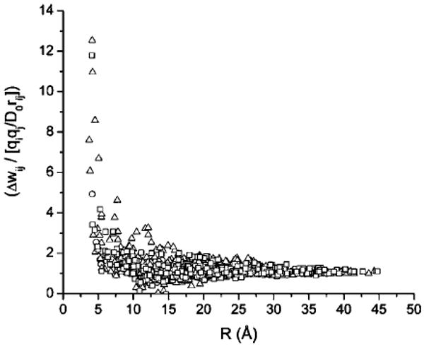
The ratio of the PMF Δwij to the Coulombic energy (uCL = qiqj/D0 rij) as a function of the distance between pairs of ionizable residues (i,j) is plotted for BPTI (open circles), HEWL (open squares), and RNase A (open triangles).
It should be noted that, in the range of 10 > rij > 20 Å, the PMF values for some charged surface groups i,j are over-screened. In other words, they have an effective dielectric constant larger than the water solvent dielectric constant D0. A similar effect was found for the PMF between charged LYS+-LYS+ pairs at positions (1,3), (1,6), and (1,7) of α-helical polylysine, which interact through the low dielectric protein cavity, calculated on the basis of a finite difference solution of the Poisson equation.35,36 It should be noted that the generalized Born (GB) approximation37–39 cannot reproduce such an overscreening effect between two charges, as shown in ref 38 because the GB approximation is a smooth interpolation of the effective dielectric constant between two limits, that is, Di and D0.
Table 7 shows the results of calculations of the ionization constants pKa for the ionizable residues of BPTI for different values of the dielectric constant DI of the protein with and without 1:1 salt effects. From Table 7, it can be seen that the calculated pKacal's are sensitive to the value of the protein dielectric constant DI. The 1:1 salt corrections, from eqs 35, 38, and 39 [column (pKacal)e in Table 7] show improvement of the agreement between the calculated pKacal values and the experimental, pKaexp, as indicated by both the average absolute deviation, Δav = 0.3, and the maximum absolute error in the pKa's, Δmax = 0.8, with respect to the same values calculated without salt [see Table 7, (pKacal)d columns]. For BPTI, better agreement is obtained between pKacal and pKaexp for DI = 16. This value is close to the values of the protein dielectric constant DP ∼ 15 found by direct simulations of the dielectric response of the protein molecule in water solution.41 The necessity to use a high value for the protein dielectric constant, namely, ∼20, to obtain results for pKa which are comparable to experimental data has been pointed out in a number of publications.9,12,49–51 The results of the calculations presented here for the pKa's, in Table 7, are in a good agreement with experimental data, as indicated by the average absolute deviation, Δav = 0.3 and the maximum absolute error in pKa's, Δmax = 0.8 pK units. In particular, this accuracy is better than the one reported by Antonisiewitcz et al.50 for the same system, namely, BPTI, as shown in Table 7, footnote f. Their results were obtained by using the standard two-dielectric continuum model and the finite difference method for solution of the linear Poisson–Boltzmann equation for electrostatic calculations in a water solution of a 1:1 salt and a detailed model for atomic charges of ionized and neutral groups. The method of Demchuck and Wade51 shows an accuracy similar to that of the present work. However, the Demchuck and Wade method assigns a different dielectric constant for different ionizable groups of the protein in order to improve the accuracy. On the other hand, the recent empirical method of Li et al.52 shows large errors in the predictions of the pKa's for BPTI.
TABLE 7. Comparison Between Computed and Observed pKa's in BPTIa.
| residue | (pKa0)b | (pKaexp)c | (pKacal)d | (pKacal)e | (pKa)f | (pKa)g | (pKa)h | ||||||
|---|---|---|---|---|---|---|---|---|---|---|---|---|---|
| DI = 2 | DI = 4 | DI = 8 | DI = 16 | DI = 2 | DI = 4 | DI = 8 | DI = 16 | ||||||
| NEND1 | 7.5 | 8.1 | 5.3 | 6.5 | 7.1 | 7.6 | 5.8 | 6.6 | 7.2 | 7.3 | 7.2 | 7.5 | – |
| ARG1 | 12.0 | – | 12.8 | 16.1 | 15.8 | 15.4 | 12.8 | 15.6 | 14.8 | 14.5 | 18.1 | 13.6 | – |
| ASP3i | 4.0 | 3.0 | 1.8 | 1.8 | 1.9 | 2.0 | 2.4 | 2.5 | 3.3 | 3.2 | 3.4 | 3.3 | – |
| GLU7 | 4.4 | 3.7 | 14.9 | 6.1 | 4.1 | 2.9 | 14.4 | 6.4 | 5.3 | 4.1 | 5.4 | 3.7 | – |
| TYR10 | 9.6 | – | 12.7 | 9.5 | 8.8 | 8.5 | 12.5 | 9.6 | 9.4 | 9.2 | 9.9 | 9.6 | – |
| LYS15 | 10.4 | 10.6 | 9.4 | 10.4 | 10.8 | 10.8 | 9.9 | 10.4 | 10.7 | 10.6 | 10.4 | 10.5 | – |
| ARG17 | 12.0 | – | 12.2 | 12.6 | 12.6 | 12.6 | 12.0 | 12.4 | 12.3 | 12.0 | 12.2 | 12.2 | – |
| ARG20 | 12.0 | – | 9.4 | 12.8 | 13.4 | 13.5 | 9.5 | 12.6 | 12.6 | 12.7 | 13.1 | 12.9 | – |
| TYR21 | 9.6 | – | 12.6 | 10.5 | 9.7 | 9.4 | 12.5 | 10.7 | 9.9 | 9.7 | 10.1 | 9.5 | – |
| TYR23 | 9.6 | – | 21.5 | 13.0 | 10.2 | 9.5 | 21.2 | 13.0 | 10.2 | 9.7 | 11.3 | 10.6 | – |
| LYS26 | 10.4 | 10.6 | 10.5 | 10.7 | 11.1 | 10.9 | 10.6 | 10.8 | 10.8 | 10.7 | 10.4 | 10.6 | – |
| TYR35 | 9.6 | – | 17.1 | 10.9 | 8.8 | 8.1 | 16.8 | 11.1 | 9.5 | 8.9 | 9.5 | 8.5 | – |
| ARG39 | 12.0 | – | 11.9 | 12.8 | 12.9 | 12.8 | 11.8 | 12.5 | 12.2 | 12.2 | 12.2 | 12.4 | – |
| LYS41 | 10.4 | 10.8 | 8.8 | 11.3 | 11.5 | 11.4 | 9.0 | 11.3 | 11.2 | 11.1 | 10.2 | 10.8 | – |
| ARG42 | 12.0 | – | 11.8 | 12.9 | 12.9 | 12.9 | 11.7 | 12.6 | 12.1 | 12.1 | 13.0 | 12.5 | – |
| LYS46 | 10.4 | 10.6 | 8.9 | 9.8 | 10.2 | 10.6 | 9.3 | 9.9 | 10.3 | 10.4 | 10.0 | 10.3 | – |
| GLU49 | 4.4 | 3.8 | 4.4 | 3.6 | 3.5 | 3.2 | 4.9 | 4.3 | 4.3 | 4.1 | 3.8 | 3.7 | – |
| ASP50 | 4.0 | 3.4 | 1.8 | 1.5 | 1.8 | 2.4 | 2.5 | 2.5 | 2.7 | 2.6 | 2.3 | 2.6 | – |
| ARG53 | 12.0 | – | 15.1 | 14.7 | 14.2 | 13.9 | 14.8 | 14.3 | 13.3 | 13.1 | 12.9 | 13.0 | – |
| CEND58 | 3.8 | 2.9 | 1.5 | 1.7 | 1.8 | 2.1 | 2.3 | 2.4 | 3.0 | 2.9 | 3.9 | 3.3 | – |
| (Δav)j | 2.5 | 1.0 | 0.8 | 0.6 | 2.0 | 0.8 | 0.5 | 0.3 | 0.7 | 0.3 | 0.6 | ||
| (Δmax)k | 3.2 | 2.4 | 1.6 | 1.0 | 3.1 | 2.7 | 1.4 | 0.8 | 1.7 | 0.8 | 1.5 | ||
In pK units, computed by eq 18.
Value of pKa0 of the residues at T = 300 K.51
Experimental values of pKaexp for the residue in 0.2 M NaCl and at T = 300 K.51
Calculated pKa for BPTI using D0 = 80 and DI = 2, 4, 8, and 16 in 0.0 M salt at T = 300 K.
Calculated pKa for BPTI using D0 = 80 and DI = 2, 4, 8, and 16 in 0.15 M of 1.1 salt at T = 300 K.
Calculated in ref 50 at 0.15 M ionic strength and T = 293 K.
Calculated in ref 51.
Calculated in ref 52. Dashes indicate that the pKa's for these ionizable groups were not reported in ref 52.
Average value of the absolute difference between observed and computed pKa's.
Maximum deviation between observed and computed pKa's.
The optimal value of 16 for DI, obtained for BPTI, has been adopted for the remaining tests on HEWL and RNase A.
Proteins HEWL and RNase A
HEWL
The calculated ionization constants pKa of lysozyme (HEWL) and ribonuclease (RNase A) are shown in Tables 8 and 9, respectively. It can be seen in Table 8 that the average absolute deviation from the experimental pKa's, Δav, is equal to 0.5 pK units for HEWL and that the maximum deviation, Δmax, is equal to 1.2 pK units. The achieved accuracy is better than those of other methods for the same protein12,50–52 (see (Δav) and (Δmax) in Table 8). Six residues, namely, GLU7, ASP18, GLU35, TYR53, ASP66, and ASP119, have the largest shift for pKaexp with respect to the corresponding pKa0, namely, more than 1.5 pK units. For these six residues (indicated with the superscript j in Table 8), the average absolute deviation (Δav) of the calculated values, pKacal, from the experimental data, pKaexp, is 0.7 pK units.
TABLE 8. Comparison Between the Computed and Observed pKa in HEWLa.
| residue | (pKa0)b | (pKaexp)c | (ΔpK(1))d | (pKacal)e | (pKa)f | (pKa)g | (pKa)h | (pKa)i |
|---|---|---|---|---|---|---|---|---|
| NEND1 | 7.5 | 7.9 | −0.89 | 6.8 | 5.6 | 8.2 | 7.3 | – |
| LYS1 | 10.4 | 10.7 | −0.36 | 10.5 | 10.1 | 10.6 | 10.5 | – |
| ARG5 | 12.0 | – | 0.14 | 12.4 | 12.8 | – | 12.8 | – |
| GLU7j | 4.4 | 2.6 | −0.06 | 3.4 | 2.8 | 2.6 | 2.9 | 3.7 |
| LYS13 | 10.4 | 10.5 | 0.38 | 11.5 | 10.7 | 11.6 | 10.8 | – |
| ARG14 | 12.0 | – | −0.10 | 12.3 | 12.4 | – | 12.6 | – |
| HIS15 | 6.6 | 5.8 | −0.26 | 5.9 | 5.1 | 5.4 | 5.8 | – |
| ASP18j | 4.0 | 2.0–2.9 | 0.09 | 3.6 | 2.7 | 3.4 | 2.6 | – |
| TYR20 | 9.6 | 10.3 | 1.71 | 9.8 | 12.4 | 13.0 | 11.8 | – |
| ARG21 | 12.0 | – | 0.26 | 13.2 | 12.7 | 13.2 | – | |
| TYR23 | 9.6 | 9.8 | 0.48 | 9.3 | 9.7 | 10.0 | 9.4 | – |
| LYS33 | 10.4 | 10.6 | 0.04 | 10.4 | 10.9 | 11.1 | 10.5 | – |
| GLU35j | 4.4 | 6.1 | 0.58 | 5.0 | 5.6 | 4.6 | 4.5 | 5.0 |
| ARG45 | 12.0 | – | −0.65 | 11.7 | 12.2 | – | 12.4 | – |
| ASP48 | 4.0 | 3.4–4.3 | 0.50 | 3.4 | 1.5 | 1.3 | 2.7 | 1.4 |
| ASP52 | 4.0 | 3.5 | −0.39 | 3.3 | 3.6 | 5.4 | 3.0 | – |
| TYR53j | 9.6 | 12.1 | 0.41 | 12.5 | 20.5 | 16.0 | 11.9 | – |
| ARG61 | 12.0 | – | −0.18 | 13.4 | 13.7 | – | 13.1 | – |
| ASP66j | 4.0 | 1.9 | 1.05 | 3.0 | 1.9 | 1.5 | 2.9 | 1.3 |
| ARG68 | 12.0 | – | −0.44 | 13.8 | 13.0 | – | 13.3 | – |
| ARG73 | 12.0 | – | 0.14 | 12.3 | 12.5 | – | 12.5 | – |
| ASP87 | 4.0 | 2.1–3.7 | −0.20 | 2.6 | 2.4 | 0.5 | 2.3 | – |
| LYS96 | 10.4 | 10.7 | 0.35 | 11.3 | 13.6 | 11.8 | 11.2 | – |
| LYS97 | 10.4 | 10.2 | 0.07 | 11.4 | 11.2 | 11.4 | 11.1 | – |
| ASP101 | 4.0 | 4.3 | 0.98 | 3.9 | 4.4 | 6.9 | 3.8 | – |
| ARG112 | 12.0 | – | −0.24 | 12.2 | 11.2 | – | 12.4 | – |
| ARG114 | 12.0 | – | 0.04 | 12.2 | 13.3 | – | 12.5 | – |
| LYS116 | 10.4 | 10.3 | −0.21 | 10.3 | 9.3 | 10.4 | 10.4 | – |
| ASP119j | 4.0 | 2.5 | 0.04 | 2.9 | 3.7 | 3.1 | 2.8 | – |
| ARG125 | 12.0 | – | −0.05 | 12.8 | 12.9 | – | 12.6 | – |
| ARG128 | 12.0 | – | 0.13 | 12.4 | 12.2 | – | 12.3 | – |
| CEND129 | 3.8 | 3.0 | −0.09 | 2.8 | 3.1 | 2.9 | 2.6 | |
| (Δav)k | 0.5 (0.7)m | 1.0 | 1.0 | 0.5 | 0.7 | |||
| (Δmax)l | 1.2 (1.1)n | 2.9 | 2.7 | 1.6 | 1.7 |
In pK units, computed by eq 18 with DI = 16, 0.15 M salt concentration at T = 300 K.
Value of pKa0 of the residues at 300 K.51
Experimental values of pKaexp for the residues in 0.15 M NaCl and at T = 300 K.12
ΔpK(1) is the shift in pKa0 due to the transport of the ionizable residue from the solution into the protein and is computed by using eq 28.
Calculated pKa for HEWL by using D0 = 80, DI = 16, and 0.10 M 1:1 salt, at T = 300 K.
Calculated in ref 50.
Calculated in ref 12. Dashes indicate that the pKa's for these ionizable groups were not reported in ref 12.
Calculated in ref 51.
Calculated in ref 52. Dashes indicate that the pKa's for these ionizable groups were not reported in ref 52.
Average value of the absolute difference between observed and computed pKa's.
Maximum deviation between observed and computed pKa's.
Average value of the absolute difference between observed and computed pKa's only for those residues indicated by footnote j in column 1.
Maximum deviation between observed and computed pKa's only for those residues indicated by footnote j in column 1.
TABLE 9. Comparison Between the Computed and Observed pK in RNase Aa.
| residue | (pKa0)b | (pKaexp)c | (ΔpK(1))d | (pKacal)e | (pKacal)f | (pKacal)g | (pKa)h | (pKa)i | (pKa)j | (pKa)k | (pKa)l |
|---|---|---|---|---|---|---|---|---|---|---|---|
| NEND1 | 7.5 | 7.6 | 0.05 | 7.0 | 7.1 | 7.0 | 6.3 | 7.1 | – | – | – |
| LYS1 | 10.4 | – | 0.01 | 10.7 | 10.8 | 10.7 | 10.5 | 10.6 | – | – | – |
| GLU2m | 4.4 | 2.8 | 0.62 | 1.3 | 3.2 | 3.0 | 2.0 | 2.6 | 2.6 | 0.0 | 2.4 |
| LYS7 | 10.4 | – | −0.34 | 9.9 | 10.7 | 10.1 | 9.6 | 10.7 | – | – | – |
| GLU9 | 4.4 | 4.0 | 0.04 | 3.9 | 4.1 | 3.9 | 4.7 | 4.3 | – | 2.6 | 2.8 |
| ARG10 | 12.0 | – | −0.24 | 14.8 | 12.6 | 12.3 | 17.6 | 13.7 | – | – | – |
| HIS12 | 6.6 | 6.2 | −0.31 | 4.8 | 6.0 | 4.8 | 4.2 | 6.2 | 5.8 | 5.1 | 6.6 |
| ASP14m | 4.0 | 2.0 | 1.22 | 2.1 | 1.8 | 1.9 | 0.0 | 2.3 | 1.7 | 3.1 | 0.8 |
| TYR25 | 9.6 | – | 1.65 | 16.0 | 16.1 | 16.1 | 19.6 | 15.0 | – | – | – |
| LYS31 | 10.4 | – | −0.28 | 10.3 | 10.3 | 10.3 | 9.7 | 10.2 | – | – | – |
| ARG33 | 12.0 | – | 0.24 | 13.5 | 13.7 | 13.7 | 13.4 | 13.7 | – | – | – |
| LYS37 | 10.4 | – | −0.04 | 10.9 | 11.0 | 11.0 | 10.9 | 11.0 | – | – | – |
| ASP38 | 4.0 | 3.1 | 0.10 | 2.9 | 3.0 | 2.9 | 3.2 | 2.8 | – | 1.5 | 2.2 |
| ARG39 | 12.0 | – | −0.12 | 12.4 | 12.7 | 12.5 | 12.5 | 12.9 | – | – | – |
| LYS41 | 10.4 | – | −0.98 | 8.8 | 8.9 | 8.5 | 9.7 | 9.3 | – | – | – |
| HIS48 | 6.6 | 6.3 | −1.33 | 7.3 | 7.2 | 7.4 | 9.7 | 4.9 | – | 6.3 | 8.3 |
| GLU49 | 4.4 | 4.7 | 0.67 | 4.8 | 4.7 | 4.8 | 5.4 | 5.1 | – | 5.0 | 3.7 |
| ASP53 | 4.0 | 3.9 | 0.18 | 3.9 | 3.9 | 3.9 | 3.9 | 3.5 | – | 3.8 | 3.6 |
| LYS61 | 10.4 | – | 0.31 | 11.4 | 11.1 | 11.4 | 10.4 | 11.2 | – | – | – |
| LYS66 | 10.4 | – | 0.05 | 11.7 | 11.7 | 11.6 | 12.6 | 11.4 | – | – | – |
| TYR73 | 9.6 | – | 1.13 | 11.6 | 11.6 | 11.6 | 14.0 | 11.0 | – | – | – |
| TYR76 | 9.6 | – | 0.74 | 9.9 | 9.7 | 9.8 | 10.3 | 10.1 | – | – | – |
| ASP83 | 4.0 | 3.5 | 1.39 | 3.0 | 2.9 | 3.1 | 1.7 | 1.8 | – | −0.9 | 2.2 |
| ARG85 | 12.0 | – | −0.05 | 13.3 | 13.2 | 13.3 | 13.2 | 13.2 | – | – | – |
| GLU86 | 4.4 | 4.1 | 0.67 | 4.1 | 4.3 | 4.1 | 4.7 | 3.4 | – | 3.9 | 3.2 |
| LYS91 | 10.4 | – | −0.02 | 10.7 | 10.8 | 10.8 | 11.2 | 11.0 | – | – | – |
| TYR92 | 9.6 | – | 0.86 | 9.8 | 9.8 | 9.8 | 10.8 | 10.4 | – | – | – |
| TYR97 | 9.6 | – | 2.37 | 13.6 | 13.9 | 13.8 | 17.6 | 12.7 | – | – | – |
| LYS98 | 10.4 | – | 0.06 | 10.5 | 10.4 | 10.4 | 10.2 | 10.5 | – | – | – |
| LYS104 | 10.4 | – | 0.55 | 11.9 | 10.7 | 11.9 | 10.7 | 11.3 | – | – | – |
| HIS105 | 6.6 | 6.6 | 0.66 | 7.8 | 7.6 | 7.8 | 5.6 | 6.6 | – | 7.3 | 8.3 |
| GLU111 | 4.4 | 3.5 | −0.14 | 3.7 | 3.7 | 3.5 | 4.2 | 3.7 | – | 3.7 | 3.3 |
| TYR115 | 9.6 | – | 1.12 | 12.3 | 12.6 | 12.3 | 10.8 | 10.1 | – | – | – |
| HIS119 | 6.6 | 6.1 | −0.68 | 7.5 | 6.8 | 6.3 | 6.3 | 6.2 | – | 5.7 | 6.8 |
| ASP121 | 4.0 | 3.1 | 0.76 | 0.7 | 2.9 | 2.6 | 1.1 | 2.1 | 3.7 | 0.4 | 1.0 |
| CEN124m | 3.8 | 2.4 | 0.39 | 2.4 | 2.6 | 2.3 | 2.3 | 2.4 | 0.0 | 1.6 | |
| (Δav)n | 0.7 | 0.4 | 0.4 | 1.1 | 0.5 | 0.7 | 1.3 | 1.0 | |||
| (Δmax)o | 2.4 | 1.0 | 1.4 | 3.4 | 1.7 | 1.2 | 4.4 | 2.1 |
In pK units, computed by eq 18 with DI = 16, 0.15 M salt concentration at T = 300 K.
Value of pKa0 of the residues at 300 K.51
Experimental values of the pKaexp for the residues in 0.15 M NaCl and at T = 300 K.51
ΔpK(1) is the shift in pKa0 due to the transport of the ionizable residue from the solution into the protein and is computed by using eq 28.
Calculated pKa for RNase A with the SO42– ion taken with an occupancy of 0.57 and the HIS119 taken in position A. The calculation was carried out for D0 = 80, DI = 16, 0.15 M 1:1 salt, and at T = 300 K.
Calculated pKa for RNase A with the SO42– ion taken with an occupancy of 0.57, the HIS119 taken in position B, and with the ionized group of ARG10 displaced by about 1.5 Å, resulting in rupture of the GLU2–···ARG10+ hydrogen bond. The calculation was carried out for D0 = 80, DI = 16, 0.15 M 1:1 salt, and at T = 300 K.
Calculated pKa for the same structure as described in footnote f but with the SO42– ion removed.
Calculated in ref 49.
Calculated in ref 51.
Calculated in ref 52. Dashes indicate that the pKa's for these ionizable groups were not reported in ref 52.
Calculated in ref 20. Dashes indicate that the pKa's for these ionizable groups were not reported in ref 20.
Calculated in ref 22. Dashes indicate that the pKa's for these ionizable groups were not reported in ref 22.
Average value of the absolute difference between observed and computed pKa's.
Maximum deviation between observed and computed pKa's.
RNase A
The results for RNase A (PDB code 3RN3), shown in Table 9, were obtained by considering both the SO42− ion and two alternative, observed side-chain positions of HIS119, namely, positions A and B, shown in Figure 3. Positions A and B of HIS119, as computed from their PDB coordinates, have different torsion angles χ1, namely, 158.5 and −72.6°, respectively. In position A, HIS119 is involved in a hydrogen bond with ASP121, and the distance between atoms NE2 of HIS119 and OD1 of ASP121 is equal to 2.59 Å. On the other hand, in position B, HIS119 is exposed to the solvent, and the hydrogen bond between NE2 of HIS119 and OD1 of ASP121 is broken. In both positions, HIS119 interacts electrostatically with the SO42− ion. In the structures reported in the PDB, the SO42− ion was bound to the protein surface at 57% occupancy in both positions A and B. Both conformations, namely, with HIS119 in positions A or B, were used to compute the pKa shifts. Without considering HIS119 in position B, the computed pKacal values are significantly less accurate, as shown in column (pKacal)e (Δav = 0.7, Δmax = 2.4). In fact, the best average deviation computed with HIS119 in position B gave a Δav equal to 0.4 and Δmax = 1.0 pK unit, as shown in column (pKacal) f of Table 9. The results presented in columns (pKacal)e, (pKacal) f, and (pKacal)g in Table 9 show the importance of taking into account the counterion SO42− and the conformational mobility of the protein structure, that is, through multiple positions of HIS119, for the calculation of the pK 's. Taking HIS119 in the B position, the hydrogen bond between the surface residues HIS119 and ASP121 is disrupted. This should not be unexpected since, in water, this hydrogen bond is probably unstable primarily because of exchange with neighboring water molecules. Moreover, a small conformational move of the side chain of ARG10 also disturbs the hydrogen bond between GLU2 and ARG10. Breaking the hydrogen bond between GLU2 and ARG10 induces changes of the pKa's of the partners, as shown by comparing columns (pKacal)e and (pKacal)f of Table 9 for GLU2 and ARG10 and also for HIS119 and ASP121; for example, the pKa of GLU2 is shifted down, and the pKa of ARG10 is shifted up by formation of the hydrogen bond. In general, such shifts upon formation of a hydrogen bond were predicted in ref 2. Such up/down shifts are as large as ∼2 pK units. The SO42− ion decreases the pKa's of the neighboring residue HIS12, at the distance of ∼4.5 Å, by about 1.2 pK units and affects other more distant residues (such as GLU86, HIS119, and ASP121) in the range of 0.2–0.4 pK units. It should be noted that recent methods,20–22 which combine molecular dynamics with ionization equilibrium calculations, do not lead to better accuracy for predicted pKa's for RNase A; the values reported22 for Δav and Δmax are equal to 1.0 and 2.1 pK units, respectively.
Figure 3.
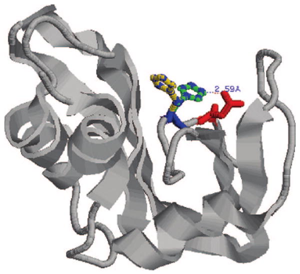
Structure of RNase A (PDB code 3RN3), showing two positions of the side chain of HIS119. In position A (blue), NE2 is hydrogen-bonded to OD1 of ASP121 (red) within 2.59 Å. In the alternative position B, this hydrogen bond does not exist.
Calculation of the pH-Dependent Ionization Free Energy
The pH-dependent ionization free energy was calculated from a direct summation over all ionization states, as given by the partition function in eq 9, only for protein BPTI, while the Tanford–Schellman integration method, eqs 12 and 16, was used for BPTI, HEWL, and RNase A. The partition function method cannot be used for HEWL and RNase A because these proteins contain more than 25 ionizable groups, as shown in Tables 7–9. The calculated ionization free energies are shown in Figure 4. A comparison of the calculations of by different methods enabled us to test the self-consistency and accuracy of the Tanford–Schellman method. From Figure 4, for example, it can be seen that, for BPTI, there is good agreement between the exact computation of the free energy, that is, calculated from the partition function, and the results of the Tanford–Schellman integral method by using both intervals of integration, namely, (−∞, pH) and (+∞, pH). The pH-dependent free energies of ionization of BPTI, calculated by the back and forth integrals (+∞, pH) and (−∞, pH), respectively, differ within only 0.2 kcal/mol and are equal to the exact free energy, calculated from the partition function, within a difference of only 1.2 kcal/mol. The differences between the back and forth ionization free energy for lysozyme and RNase are within 0.4 kcal/mol. From this analysis, we conclude that the implemented Monte Carlo method of calculation of the free energy of ionization by the Tanford–Schellman integral gives reasonable accuracy for pH-dependent effects in proteins. The calculations of the average ionization degrees 〈ɀi(x,pH)〉 of residues (by eq 11) were carried out with a Monte Carlo (MC) random walk in the ionization microstate space, that is, by partitioning the pH range of integration given by eqs 12 and 16, for example, between −25 and 25 pH units, in small increments, that is, ΔpH = 0.25. Since the ionization microstates at extremely large and low pH values are known, the MC titration method coupled with small pH increments constitutes an accurate approximation since it enables us to explore the ionization microstates more efficiently.
Figure 4.
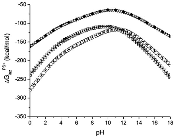
The free energy of ionization as a function of pH is shown for the proteins BPTI, HEWL, and RNase A. The upper curve shows the results obtained for BPTI (the black-filled diamonds represent the values computed by using the exact partition function, while the open up and down triangles are the result of calculations using the Tanford–Schellman integral approach after back and forth integration intervals, respectively). The results obtained for HEWL are shown in the middle curve (the squares, and dots within them, represent the results of the calculations using the Tanford–Schellman integral approach over back and forth integration intervals, respectively). The results obtained for RNase A are shown in the lower curve (the circles, and the dots within them, represent the results of the calculations using the Tanford–Schellman integral approach over back and forth integration intervals, respectively).
The relative stability of the pH-dependent ionization free energy, ΔΔGinz(x,pH), shown in Figure 5, was computed by using eq 13, which describes the ionization free energy of the folded protein conformation with respect to the unfolded reference state , in which all ionizable groups are well exposed to solvent and do not have electrostatic interactions between them. It can be seen from Figure 5 that the calculated ionization free energy stabilizes the respective native structures [ΔΔGinz(x, pH) > 0] in the pH range of ∼4 to ∼10 for BPTI, ∼5 to ∼7.5 for RNase A, and ∼7 to ∼9.5 for HEWL. For the particular case of HEWL, the calculated stabilization ΔΔGinz(x,pH) in this pH range is in good agreement, that is, within ∼2 kcal/mol, with the experimental free energy of stabilization in the pH range of ∼4 to ∼6. Although the calculated pH of maximum stability is shifted with respect to the experimental one ,53 the pH range for which the structure is stable is in qualitative agreement, for example, and , between the calculated and experimental free energy of stabilization (see Figure 5). It is worth noting that the experimental pH-dependent relative stability for HEWL was calculated with the Tanford–Schellman integral method from the experimental average ionization charge53 at 0.1 M salt concentration and 298 K, which is shown in Figure 6. In this figure, the calculated total charge as a function of the pH, , is also shown. The results indicate that, in the pH range of 4–10, in which there is an ensemble of different ionization states, the calculated charge (shown with small black-filled squares) is lower than the experimental charge (shown with large black-filled diamonds), which are both in the charge range of +6 to +10 units. Conceivably, a possible explanation of the systematic low charge for in this pH range is due to a nonlinear effect or specific counterion effects, which are not included in the current method.
Figure 5.
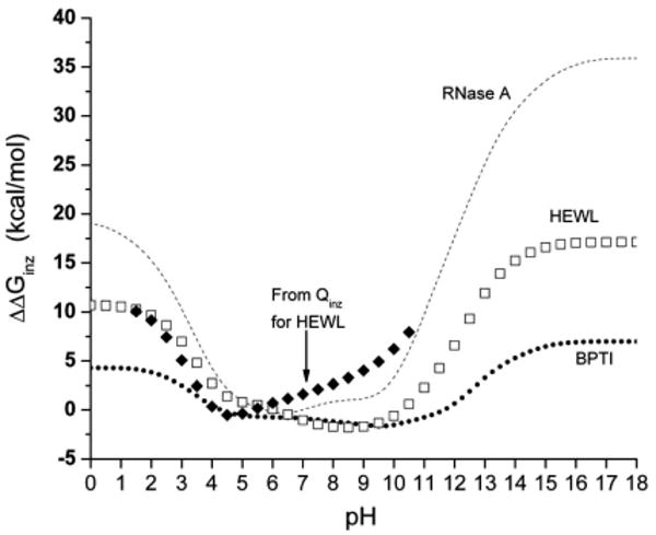
The computed stabilization free energy of ionization (ΔΔGinz, eq 13) of the native structure with respect to the non-native (unfolded one), as a function of pH, is shown for three proteins, namely, BPTI, HEWL, and RNase A. For the non-native representation of the protein structure, the average ionization was approximated by of eq 14. The dotted line is the result for BPTI, the dashed line is for RNase A, and the open squares are for HEWL. The black-filled diamonds represent the computed ΔΔGinz from the observed titration curve, Qinz(pH) (see Figure 6), only for HEWL.
Figure 6.
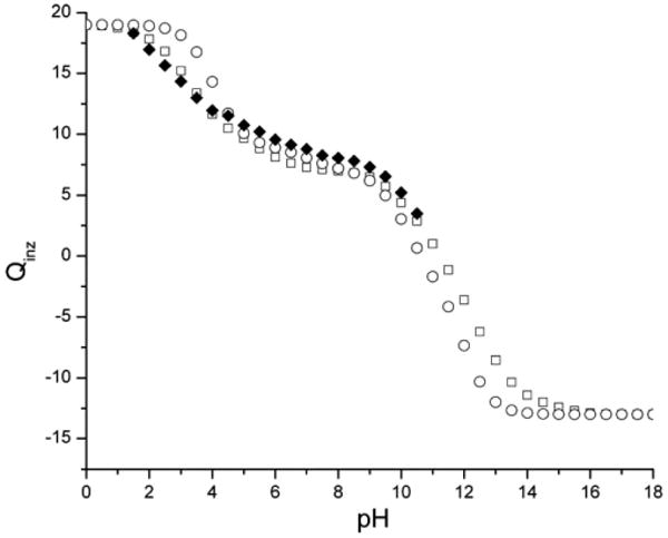
The pH-dependent total ionization charge for HEWL is shown as small black-filled squares for the curve computed by the FAMBE-pH method, the observed 53 as large black-filled diamonds, and the curve for free groups in solution as open circles.
Conclusion
The FAMBE-pH method, described for the calculation of the pH-dependent properties of proteins, is based on the dielectric continuum model of a protein in a water solvent and on the efficient boundary element method FAMBE to solve the Poisson equation taking into account 1:1 salt effects. The FAMBE-pH method shows internal self-consistency and is faster and more accurate to compute pH-dependent properties in proteins than existing methods.6–9,12,22,25,49–54 Moreover, it can also be implemented together with any existing force field to study a variety of applications such as protein stability, protein folding, and protein–ligand binding. However, it should be noted that, despite the good accuracy for the prediction of pKa's for ionizable residues, that is, with an average error of ∼0.5 pH unit for lysozyme (as shown in Table 8), such accuracy is not good enough for a precise prediction of the pH value of maximum stability in a protein such as lysozyme (as shown in Figure 5). In addition, the importance of considering the counterion effect was shown in Table 9 for RNase A. Here, it was shown that counterion effects become a significant contribution if the pH is far from the isoelectric point, and such effects certainly cannot be ignored for an accurate treatment of pH-dependent protein stability. We have also been able to show (Table 9) that, taking the conformational mobility of the protein side chains into account, for example, by considering small changes of ∼2–3 Å, could lead to significant changes in the hydrogen bond network. Such changes in the hydrogen bond network might be very important for calculating pH-dependent phenomena, as was shown for RNase A.
The solvent polarization free energy of the protein 1FCS (fasciculin II, consisting of 153 residues) was computed by Lu and McCammon55 in ∼20 s on a 2 GHz Pentium IV computer by using an improved boundary element method for solving the Poisson–Boltzmann equation at 0.0 M salt concentration. We subsequently computed the solvent polarization free energy of this protein on a 2 GHz Pentium IV computer by using the FAMBE method in a comparable time. Although we cannot compare the total free energy from both laboratories because we both used different sets of charges and atomic radii, our FAMBE-pH method presented here is not limited to computing only the solvent polarization free energy but can also compute the total free energy of solvation. In addition, the FAMBE-pH method provides a very efficient and accurate computational treatment of the multiple-site titration problem for proteins containing a large number of ionizable groups, for example, 150 for a 448 residue protein 1EA1 (Table 4). As noted in the subsection “Calculation of pKa Shifts of Proteins”, our FAMBE-pH method shows internal self-consistency in the computation of the free energy of ionization and accurate prediction of the pKa shifts in three proteins, namely, BPTI, HEWL, and RNase A. Moreover, very good agreement was found for the computation of the free energy of ionization by using both the exact calculation of the partition function and the Tanford–Schellman integral method.
All of the accumulated results indicate that the FAMBE-pH method presented here could lead to a more realistic treatment of pH-dependent phenomena, when used together with molecular dynamics or Monte Carlo conformational sampling.
Acknowledgments
This work are supported by the Russian Academy of Sciences and the Russian Fund for Basic Research, Grant 05-04-48322 (Y.V.) and by grants from the National Science Foundation (MCB05-41633) and the National Institutes of Health (GM-14312 and GM-24893). Support was also received from the National Research Council of Argentina (CONICET), FONCyT-ANPCyT (PAE 22642/22672), and from the Universidad Nacional de San Luis [UNSL] (P-328501), Argentina. The authors are grateful to J. Hermans for providing the Sigma program.
References and Notes
- 1.Rost B, Sander C. J Mol Biol. 1993;232:584. doi: 10.1006/jmbi.1993.1413. [DOI] [PubMed] [Google Scholar]
- 2.Laskowski M, Scheraga HA. J Am Chem Soc. 1954;76:6305. [Google Scholar]
- 3.Hill TL. J Am Chem Soc. 1956;78:5527. [Google Scholar]
- 4.Tanford C, Kirkwood JG. J Am Chem Soc. 1957;79:5333. [Google Scholar]
- 5.Warshel A. Biochemistry. 1981;20:3167. doi: 10.1021/bi00514a028. [DOI] [PubMed] [Google Scholar]
- 6.Bashford D, Karplus M. Biochemistry. 1990;29:10219. doi: 10.1021/bi00496a010. [DOI] [PubMed] [Google Scholar]
- 7.Beroza P, Fredkin DR, Okamura MY, Feher G. Proc Natl Acad Sci U S A. 1991;88:5804. doi: 10.1073/pnas.88.13.5804. [DOI] [PMC free article] [PubMed] [Google Scholar]
- 8.Yang AS, Gunner MR, Sampogna R, Sharp K, Honig B. Proteins: Struct, Funct, Genet. 1993;15:252. doi: 10.1002/prot.340150304. [DOI] [PubMed] [Google Scholar]
- 9.Antosiewicz J, McCammon JA, Gilson MK. J Mol Biol. 1994;238:415. doi: 10.1006/jmbi.1994.1301. [DOI] [PubMed] [Google Scholar]
- 10.Ripoll DR, Vorobjev YN, Liwo A, Vila JA, Scheraga HA. J Mol Biol. 1996;264:770. doi: 10.1006/jmbi.1996.0676. [DOI] [PubMed] [Google Scholar]
- 11.Zhou HX, Vijayakumar M. J Mol Biol. 1997;267:1002. doi: 10.1006/jmbi.1997.0895. [DOI] [PubMed] [Google Scholar]
- 12.Alexov EG, Gunner MR. Biophys J. 1997;72:2075. doi: 10.1016/S0006-3495(97)78851-9. [DOI] [PMC free article] [PubMed] [Google Scholar]
- 13.Ripoll DR, Vila JA, Scheraga HA. J Mol Biol. 2004;339:915. doi: 10.1016/j.jmb.2004.04.002. [DOI] [PubMed] [Google Scholar]
- 14.Vila JA, Ripoll DR, Arnautova YA, Vorobjev YN, Scheraga HA. Proteins: Struct, Funct, Bioinf. 2005;61:56. doi: 10.1002/prot.20531. [DOI] [PubMed] [Google Scholar]
- 15.Baptista AM, Teixeira VH, Soares CM. J Chem Phys. 2002;117:41840. [Google Scholar]
- 16.Bürgi R, Kollman PA, VanGunsteren VF. Proteins: Struct, Funct, Bioinf. 2002;47:469. doi: 10.1002/prot.10046. [DOI] [PubMed] [Google Scholar]
- 17.Dlugosz M, Antosiewicz JM. Chem Phys. 2004;302:161. [Google Scholar]
- 18.Mongan J, Case DA, McCammon JA. J Comput Chem. 2004;25:2038. doi: 10.1002/jcc.20139. [DOI] [PubMed] [Google Scholar]
- 19.Leezfn MS, Salsbury FR, Jr, Brooks CL., III Proteins: Struct, Funct, Bioinfor. 2004;56:738. doi: 10.1002/prot.20128. [DOI] [PubMed] [Google Scholar]
- 20.Khandogin J, Brooks CL., III Biophys J. 2005;89:141. doi: 10.1529/biophysj.105.061341. [DOI] [PMC free article] [PubMed] [Google Scholar]
- 21.Khandogin J, Chen J, Brooks CL., III Proc Natl Acad Sci U S A. 2006;103:18546. doi: 10.1073/pnas.0605216103. [DOI] [PMC free article] [PubMed] [Google Scholar]
- 22.Khandogin J, Brooks CL., III Biochemistry. 2006;45:9363. doi: 10.1021/bi060706r. [DOI] [PubMed] [Google Scholar]
- 23.Tanford C. Adv Protein Chem. 1970;24:1. [PubMed] [Google Scholar]
- 24.Schellman JA. Biopolymers. 1975;14:999. doi: 10.1002/bip.1975.360140113. [DOI] [PubMed] [Google Scholar]
- 25.Yang SA, Honig B. J Mol Biol. 1993;231:459. doi: 10.1006/jmbi.1993.1294. [DOI] [PubMed] [Google Scholar]
- 26.Vorobjev YN, Scheraga HA. J Comput Chem. 1997;18:569. [Google Scholar]
- 27.Vorobjev YN, Almagro JC, Hermans J. Proteins: Struct, Funct, Bioinfor. 1998;32:399. [PubMed] [Google Scholar]
- 28.Sharp KA, Honig B. Annu Rev Biophys Chem. 1990;19:301. doi: 10.1146/annurev.bb.19.060190.001505. [DOI] [PubMed] [Google Scholar]
- 29.Vorobjev YN, Hermans J. Biophys J. 1997;73:722. doi: 10.1016/S0006-3495(97)78105-0. [DOI] [PMC free article] [PubMed] [Google Scholar]
- 30.Vorobjev YN, Hermans J. Biophys Chem. 1999;78:195. doi: 10.1016/s0301-4622(98)00230-0. [DOI] [PubMed] [Google Scholar]
- 31.Vorobjev YN, Hermans J. Protein Sci. 2001;10:2498. doi: 10.1110/ps.15501. [DOI] [PMC free article] [PubMed] [Google Scholar]
- 32.Landau LD, Lifshitz EM. Electrodynamics of Continuous Media Landau and Lifshitz Corse of Theoretical Physics Volume 8 Translated from the Russian. Pergamon Press; Oxford, U.K.: 1984. pp. 34–36.pp. 39 [Google Scholar]
- 33.Yoon BJ, Lenhoff AM. J Comput Chem. 1990;11:1080. [Google Scholar]
- 34.Juffer AH, Botta EFF, Bert AM, van Keulen BAM, van der Ploeg A, Berendsen HJC. J Comp Phys. 1991;97:144. [Google Scholar]
- 35.Vorobjev YN, Scheraga HA, Hitz B, Honig B. J Phys Chem. 1994;98:10940. [Google Scholar]
- 36.Vorobjev YN, Scheraga HA, Honig B. J Phys Chem. 1995;99:7180. [Google Scholar]
- 37.Qiu D, Shenkin PS, Hollinger FP, Still WC. J Phys Chem A. 1997;101:3005. [Google Scholar]
- 38.Sigalov G, Scheffel P, Onufriev A. J Chem Phys. 2005;122:094511. doi: 10.1063/1.1857811. [DOI] [PubMed] [Google Scholar]
- 39.Onufriev A, Case DA, Bashford D. J Comput Chem. 2002;23:1297. doi: 10.1002/jcc.10126. [DOI] [PubMed] [Google Scholar]
- 40.Scheraga HA, Katchalsky A, Alterman Z. J Am Chem Soc. 1969;91:7242. [Google Scholar]
- 41.Loffler G, Schreiber H, Steinhauser O. J Mol Biol. 1997;270:520. doi: 10.1006/jmbi.1997.1130. [DOI] [PubMed] [Google Scholar]
- 42.Nina M, Beglov D, Roux B. J Phys Chem B. 1997;101:5239. [Google Scholar]
- 43.Hummer G, Pratt LR, Garcia AE. J Phys Chem. 1995;99:14188. [Google Scholar]
- 44.Aqvist J, Hansson T. J Phys Chem. 1996;100:9512. [Google Scholar]
- 45.Hermans J. University of North Carolina; 1999. Sigma Documentation. http://hekto.med.unc.edu/HERMANS/software/SIGMA/index.html. [Google Scholar]
- 46.Berendsen HJC, Postma JPM, van Gunsteren WF, Hermans J. In: Jerusalem Symposia on Quantum Chemistry and Biochemistry. Pullmann B, editor. D Reidel; Dordrecht, The Netherlands: 1981. [Google Scholar]
- 47.Essmann U, Perera L, Berkowitz L, Darden T, Lee H, Pedersen LG. J Chem Phys. 1995;103:8577. [Google Scholar]
- 48.Sitkoff D, Sharp KA, Honig B. J Phys Chem. 1994;98:1978. [Google Scholar]
- 49.Antosiewicz J, McCammon JA, Gilson MK. Biochemistry. 1996;35:7819. doi: 10.1021/bi9601565. [DOI] [PubMed] [Google Scholar]
- 50.Antosiewicz J, Briggs JM, Elcock AH, Gilson MK. J Comput Chem. 1996;17:1633. [Google Scholar]
- 51.Demchuk E, Wade RC. J Phys Chem. 1996;100:17373. [Google Scholar]
- 52.Li H, Robertson AD, Jensen JH. Proteins: Struct, Funct, Bioinfor. 2005;61:704. doi: 10.1002/prot.20660. [DOI] [PubMed] [Google Scholar]
- 53.Tanford C, Roxby R. Biochemistry. 1972;11:2192. doi: 10.1021/bi00761a029. [DOI] [PubMed] [Google Scholar]
- 54.Schafer M, Sommer M, Karplus M. J Phys Chem B. 1997;101:1663. [Google Scholar]
- 55.Lu B, McCammon A. J Chem Theory Comput. 2007;3:1134. doi: 10.1021/ct700001x. [DOI] [PubMed] [Google Scholar]