Nonparametric Residue Analysis of Dynamic PET Data With Application to Cerebral FDG Studies in Normals

Abstract

Kinetic analysis is used to extract metabolic information from dynamic positron emission tomography (PET) uptake data. The theory of indicator dilutions, developed in the seminal work of Meier and Zierler (1954), provides a probabilistic framework for representation of PET tracer uptake data in terms of a convolution between an arterial input function and a tissue residue. The residue is a scaled survival function associated with tracer residence in the tissue. Nonparametric inference for the residue, a deconvolution problem, provides a novel approach to kinetic analysis—critically one that is not reliant on specific compartmental modeling assumptions. A practical computational technique based on regularized cubic B-spline approximation of the residence time distribution is proposed. Nonparametric residue analysis allows formal statistical evaluation of specific parametric models to be considered. This analysis needs to properly account for the increased flexibility of the nonparametric estimator. The methodology is illustrated using data from a series of cerebral studies with PET and fluorodeoxyglucose (FDG) in normal subjects. Comparisons are made between key functionals of the residue, tracer flux, flow, etc., resulting from a parametric (the standard two-compartment of Phelps et al. 1979) and a nonparametric analysis. Strong statistical evidence against the compartment model is found. Primarily these differences relate to the representation of the early temporal structure of the tracer residence—largely a function of the vascular supply network. There are convincing physiological arguments against the representations implied by the compartmental approach but this is the first time that a rigorous statistical confirmation using PET data has been reported. The compartmental analysis produces suspect values for flow but, notably, the impact on the metabolic flux, though statistically significant, is limited to deviations on the order of 3%–4%. The general advantage of the nonparametric residue analysis is the ability to provide a valid kinetic quantitation in the context of studies where there may be heterogeneity or other uncertainty about the accuracy of a compartmental model approximation of the tissue residue.

1. Introduction

The ability to image radiolabeled forms of important biological molecules with positron emission tomography (PET) has immense potential for the study and treatment of human disease (Phelps 2000). The PET reconstruction problem, introduced to statisticians by Vardi, Shepp, and Kaufman (1985), focused on the estimation of a single static image of the uptake of the radiotracer in the field of view. By following the tracer uptake, dynamic PET studies offer the opportunity to evaluate local biochemical and physiologic processes associated with the metabolism of a radiolabeled molecule. Quantitative interpretation of data from dynamic PET experiments may not be straightforward. The dynamic uptake data measured by PET scanning reflects a combination of local metabolic processes and the time-course of delivery, via the blood plasma, of the radiotracer to the local tissue. Often the time-course of the radiotracer in the plasma is affected by processes at remote organs, such as first-pass extraction and transient retention in membrane lipids. Thus PET uptake data do not merely represent the local metabolic process that is of interest and so the separation of the plasma time-course from the PET uptake data become essential. The most widely used approach is kinetic analysis with compartmental models (Cunningham, Gunn, and Matthews 2004; Huang and Phelps 1986; Mazoyer, Huesman, Budinger, and Knittel 1986; Mankoff, Muzi, and Zaidi 2005; Murase 2003). Here the metabolic processes in the tissue are represented by a series of compartments within the tissue. The compartments may represent physical regions (capillary segments, cells, etc.) or phases of biochemical transformation (unmetabolized tracer, products of tracer metabolism) that are distributed over elements within the tissue. Given the PET uptake data and a measured plasma function, the kinetic constants controlling the rate of transfer between compartments can be estimated using nonlinear weighted least squares fitting techniques. Although there are certain situations where the approach is well established, when there is limited understanding of the kinetic behavior of target tissue with respect to the radiotracer under consideration, there is a danger that interpretations of PET data obtained by compartmental kinetic analysis will be misleading.

In the PET literature one finds the two-compartment model, proposed for ¹⁸F-Fluoro-deoxyglucose (FDG) metabolism in normal brain tissue (Phelps et al.1979), being applied in circumstances with different tissues and even different radiotracers, without substantive biological support for the underlying assumptions. This is inappropriate given the high degree of complexity associated with both the biology and with the analysis of dynamic PET studies. The resolution of PET is ultimately limited by dose constraints and it is clear that the typical noise associated with PET time-course data often provides limited power to statistically discriminate between alternative model formulations for a given dataset. Thus, even though a two-compartment model may provide a satisfactory fit to a given dataset, this does not validate the biological assumptions of that model. For validation, supplementary in-vitro and in vivo experimentation is required. With FDG, the basic biochemistry of the model has been validated by test-tube experimentation (Huang et al. 1980). However, in vivo tissue data do not necessarily behave as a well-stirred test-tube and indeed tissue heterogeneity also has been raised as a particular concern; see Lucignani et al. (1993) for example. Thus the hypothesis of the FDG model even for brain tissue, where the greatest degree of validation work has been undertaken, might be questioned. In the context of exploring potential alternatives to narrowly formulated compartmental models, a general technique that includes the compartmental approach as a special case, is potentially helpful. This provides the motivation for the work presented here.

Dynamic PET data are measurements of the concentration of an isotope in tissue over time, and this data include noise from the statistical nature of radioactive decay and from the image reconstruction process. The indicator dilution theory of Meier and Zierler, reviewed and generalized in this article, focuses on the representation of PET uptake data as a convolution between the tissue residue function of the isotope and the plasma input function. Technically, the residue is a scaled survival function. Given regional PET data and a measured plasma curve, it should be possible to use deconvolution to recover an estimate of the tissue residue. A particular technique for realizing such a measurement is described here. The approach uses regularized cubic B-spline approximation of the residence time distribution and employs quadratic programming to solve for unknown coefficients. An assessment of the sampling variation in the residence time or the residue function can be obtained by simulation. Functional inferences for specific hypotheses can be developed. In particular, hypotheses of specific compartmental model representations for PET residue functions can be considered. The methodology is applied to data from a series of cerebral dynamic PET FDG studies in normal subjects (Graham et al. 2002). The data allow regional statistical comparisons to be made between analyses produced by the standard two-compartment model for FDG of Phelps et al.(1979) and the proposed nonparametric technique. Evidence of statistically significant differences between regional means of functional parameters produced by alternative analysis techniques are found. Remarkably, the impact on flux is only on the order of 3%–4% and this is of little practical significance. Substantive deviations are found in the measurement of flow. Whereas a number of factors might contribute to this result, the literature (e.g., King, Raymond, and Bassingthwaighte 1996; Ostergaard, Weisskoff, Chesler, Gyldensted, and Rosen 1996; Ostergaard, Chesler, Weisskoff, Sorensen, and Rosen 1999) does not support the assumption of exponential flow distributions in vascular networks—an essential part of the compartmental approach. The nonparametric analysis estimates residue patterns that are consistent with more realistic nonexponential lognormal type patterns. Whereas nonparametric residue analysis leads to some increased variability, this is a small price for a more accurate and consistent result. Notably, in the context of cerebral FDG, the determination of flux by the nonparametric residue approach carries only a minimal increase in variance. Overall these results are highly satisfactory and indicate that, in the absence of a well-validated compartmental kinetic model or in the presence of substantial tissue heterogeneity, direct quantitation of PET data based on functionals of nonparametrically reconstructed residues is a practical and reliable alternative.

2. Theory

In a seminal paper Meier and Zierler (1954) introduced a theoretical basis for the analysis of indicator dilution studies. This entailed the description of the residual indicator in a vascular network in terms of a survival function. Here we show how this probabilistic view of indicators is readily adapted to PET radiotracers and leads to a general connection to an associated survival function. We begin with a review of indicator dilution theory and then present the generalization to PET radiotracers. Connections between this approach and linear compartmental models are also discussed.

2.1 Vascular Tracers Without Loss

Meier and Zierler were concerned with the description of an intravascular indicator flowing through a vascular network within a tissue region. The concentration of indicator at time t, denoted C_T(t), in the tissue region is considered. Using assumptions of linearity and time-invariance, a convolution integral representation describing C_T(t) in terms of the input concentration, C_P(t), in the arterial supply to the region, was developed. The basic equation is

$$C_T(t)=K{\int }_o^{t}R(t-s)C_P(s)ds$$ (1)

where K is a proportionality constant, interpretable as an overall flow, and R(t) is the tissue residue function. Physically the residue function describes the fraction of indicator, which remains in the tissue in response to an idealized bolus (Dirac delta function) input concentration at time t = 0. Initially the residue must be unity (R(0) = 1) and from there it decreases (at least does not increase) as t increases. Assuming the residue is differentiable, it can be represented in the form

$$R(t)=1-{\int }_o^{t}h(\tau )d\tau$$ (2)

where h(τ) is a probability density function. An interpretation of h in terms of the residence time distribution associated with an ensemble of capillary transport paths within the region was developed by Meier and Zierler. Indicator molecules are assumed to randomly sample such paths. Once a path is selected, the travel time of the molecule in the tissue is determined. Either due to flow or volume variations, the transit time of the indicator in each transport path is considered to be distinct. From the distribution of transport paths there arises a distribution of transit times that would be experienced by a randomly chosen indicator molecule. The probability that an indicator molecule ends up on a path with transit time between t and t + Δt is proportional to h(t)Δt as Δt gets small. Hence if a collection of indicator molecules are introduced in trace amounts, so they do not interact, the fraction of molecules that experience transit times greater than t is given by $R(t)=1-{\int }_o^{t}h(\tau )d\tau$.

The interpretation of K as a flow, when the tracer is confined to the intravascular space, is obtained by considering the structure of the tissue concentration in response to a constant concentration in the arterial supply, C_P(t) = C_P. If the fractional vascular volume within the tissue is V_B, then the concentration in tissue will eventually equilibrate in the tissue vasculature so that the total amount in the tissue will be V_BC_P and no tracer will be distributed outside of V_B. But assuming that the residence time distribution has a finite first moment, which implies (Rao 1973) ${lim}_{t\to \infty }[1-{\int }_o^{t}h(\tau )d\tau ]t=0$, then application of integration by parts gives

$$\begin{array}{l}\underset{t\to \infty }{lim}{C}_T(t)=V_B{C}_P=K\underset{t\to \infty }{lim}{\int }_o^{t}R(t-s)C_P(s)ds\\ =K{\int }_o^{\infty }R(t)dt\cdot C_P=K{\mu }_T{C}_P\end{array}$$ (3)

where μ_T is the mean transit time over all available transport paths. Hence Kμ_T = V_B and K = (V_B / μ_T) is the net flow of the intravascular indicator through the tissue region. This relation is referred to as the central volume theorem. The theory of Meier and Zierler has been applied to develop techniques for determination of cerebral flow and volume with dynamic magnetic resonance (MR) and computerized tomography studies (Axel 1980; Keeling, Bammer, Kogler, and Stollberger 2004; Larson et al. 1994; Ostergaard et al. 1996).

2.2 General Tracers Including Loss

The distributional viewpoint underlying Meier and Zierler's approach to intravascular dilutions readily extends to indicators that pass out of the vasculature and indeed to radioactive tracers used in PET. In the case that the labeled indicator is metabolized, the fate of the label (isotope) must be considered. Suppose the tissue region presents an ensemble of possible pathways that the indicator label can follow during the course of the study. Each such pathway could entail a complex set of specific interactions with transporters, flows in microvasculature, receptor ligands, enzymes etc. that are present in the tissue. If biochemical transformation takes place on a particular pathway, then the label may become attached to a different molecular structure, which may or may not be retained in tissue. Depending on the indicator and the tissue, there may be pathways where label at the end of the study is bound to a receptor or otherwise trapped in a subcellular structure that may not even be in communication with the capillary bed of the tissue. The distribution of the entire set of pathways is a characteristic of the tracer and the tissue region.

For each pathway consider the length of time, its residence time, that the label will remain in the tissue region. The distribution of pathways within the tissue induces a probability distribution function, denoted H(·), for these residence times. If a trace quantity of labeled molecules is introduced to the tissue, the residence times of the attached labels will behave as a random sample from this distribution. Formally, because the study has limited time of duration, the sample of residence times for labeled molecules will be right censored. So if T_e represents the end of the study, then the observable residence time for a randomly selected tracer molecule label lies between 0 and T_e. Let U be an indicator that measures if the label on a particular tracer molecule has an actual residence time, T, exceeding T_e. U is a Bernoulli random variable with success probability ε = 1 − H(T_e). For t ∈ [0, T_e], the residue function is the probability that T is greater than t

$$\begin{array}{l}R(t)=P\left[T>t\right]\\ =1-H(t)\\ =1-P\left[T\le t|T\le T_e\right]P\left[T\le T_e\right]\\ =1-H_o(t)(1-\epsilon )\end{array}$$ (4)

where H_o(·) represents the conditional residence distribution of labels that have residence times less than T_e. Note the second to last step follows because since t ≤ T_e, P[T ≤ t] = P[T ≤ t and T ≤ T_e]. If H_o(·) is differentiable then $H_o(t)={\int }_o^{t}h(\tau )d\tau$ where h represents the residence time probability density for pathways with residence times less than or equal to T_e. Thus the concentration in tissue becomes

$$C_T(t)=K{\int }_o^{t}R(t-s)C_P(s)ds,$$ (5)

which looks like Equation (1) but now $R(t)=1-\zeta {\int }_o^{t}h(\tau )d\tau$ with the parameter ζ = H(T_e) = 1 − ε reflecting the proportion of tracer, which is returned from the tissue by time T_e. Following Gjedde (1987), we refer to ζ as the exchange ratio of the tissue. The fraction of indicator extracted (bound) at time T_e by the tissue is ε = 1 − ζ = R(T_e). It is important to appreciate that both ζ and ε are functions of T_e. Thus there is no way to objectively infer the nature of the residue at times after T_e. Obviously, if the measurement interval is extended then the corresponding exchange ratio may well be larger. An asymptotic assessment of extraction or exchange cannot be deduced from the data gathered in a finite time period. Meier and Zierler's theory focused on intravascular indicators. In this setting there is no net loss of indicator from the region, i.e. ζ = 1 and ε = 0.

Application of integration by parts to (5), gives that the concentration in tissue at time t in response to a constant arterial supply (C_P(t) = C_P) as

$$\begin{array}{l}{C}_T(t)=[1-\zeta H_o(t)]K{C}_{P}t+(1-\epsilon )K{\int }_o^t\tau h(\tau )d\tau C_P\\ ={\epsilon }^{(t)}K{C}_{P}t+(1-\epsilon )K{\mu }_T^{(t)}{C}_P\end{array}$$ (6)

where ε^(t) = [1 − ζH_o(t)] and ${\mu }_T^{(t)}={\int }_o^t\tau h(\tau )d\tau$. For large t (≤ T_e), because H_o(T_e) = 1, ε^(t) → ε, ${\mu }_T^{(t)}\to {\mu }_T$, the mean transit time associated with the conditional (unbound) residence and the Equation (6) becomes

$$C_T(t)\approx \epsilon K{C}_{P}t+(1-\epsilon )K{\mu }_T{C}_P$$

By analogy with a flow network with loss, K is the flow rate and εK is a flux representing the net rate of loss from the network. Because the tracer accumulates in tissue over time, the interpretation of Kμ_T as a physically measurable distribution volume, based on constant infusion, is problematic. If the residence density is partitioned into quantiles, the volumes occupied by fast, intermediate, and slow moving radiotracer label can be separately assessed. To obtain a volume that is comparable to the approach used with the two-compartment FDG model, described later, we propose a distribution volume, ${\text{V}}_D^F$, using the scaled first quantile of the residence density as the reference transit time

$${\text{V}}_D^F=K{\mu }_T^F\equiv K\frac{{\mu }_T^{[0.25]}}{log(4/3)}$$

where ${\mu }_T^{[0.25]}$ is the first quantile of the residence. The scaling ensures that if the residence density is exponential, h(t) = (1/α)e^−αt, then ${\mu }_T^F$ is equal to (1/α), the mean of the residence distribution.

2.3 Incorporation of a Blood Volume and Delay

In the case that passage through the tissue region can proceed without significant interaction with a capillary network, or that indicator molecules are extracted slowly from the vascular space, relative to the flow in the vasculature and the time resolution of acquisition, the residence distribution, H_o, may initially have an apparent jump corresponding to label attached to molecules that are effectively passed without interaction with tissue. Here H_o(·) will not be differentiable at t = 0 and it is reasonable to separately focus on the distribution for residence times strictly between 0 and T_e. The tissue concentration formula becomes:

$$C_T(t)=V_B{C}_P(t)+K{\int }_o^{t}R(t-s)C_P(s)ds$$ (7)

where V_B is the fractional volume occupied by indicator labels that are not slowed by passage through the tissue and the residue function is

$$R(t)=1-\zeta {\int }_o^{t}h(\tau )d\tau$$ (8)

with ζ = 1 − ε and h is the probability distribution of residence times in (0,T_e). For slowly metabolized indicators, V_B is effectively the fractional blood volume in the tissue.

The sampled blood plasma concentration is often undertaken at a site that is remote from the tissue region under study. Thus there are possibilities for delay and dispersion. The delay is readily incorporated. With delay, Δ, the tissue concentration formula becomes

$$C_T(t)=V_B{C}_P(t-\Delta )+K{\int }_o^{t}R(t-s)C_P(s-\Delta )ds.$$ (9)

It may also be the case that, due to dispersion in blood vessels, the plasma concentration at the measurement site may only provide a convolved view of the concentration seen at the tissue. This leads to the consideration of a correction for dispersion before analysis. Dispersion is relevant in studies where temporal sampling frequency is comparable with the scale of dispersion. For the FDG studies considered here the issue is not practically significant but for extension to fast tracers, such as water this point would need to be addressed. Important functionals of the residue are the flow, distribution volume, flux, a representative transit time (here we use the median transit time), and extraction.

2.4 Compartmental Models and their Residues

The most widely used approach for kinetic analysis of PET data are linear compartmental modeling (Cunningham et al. 2004, Mazoyer et al. 1986, Mankoff et al. 2005). In this approach, the tissue region is represented as a well-mixed volume in which tracer label is assumed to exist in a discrete number of states called compartments. Compartments associated with vascular, extracellular, and various intracellular constructs are common. A compartmental model specifies a system of (typically linear) differential equations describing the rate of transfer of tracer from one compartment to another over the time-course of the study. Solving the system of equations leads to a representation for the total tissue concentration of the tracer over time. In the case of linear compartmental models, solutions can always be expressed in the convolution form of Equation (8). In fact the residue function corresponds to the impulse response for the compartmental model. Elementary analysis shows the impulse response for a linear compartmental model is a sum of decaying exponentials. Using Equation (9) the residence density associated with a linear compartmental model is a mixtures of exponential densities.

By way of illustration, consider the two-compartment model proposed by Phelps et al. (1979) for analysis of FDG data. A schematic for this model is shown in Figure 1. The residue function, R_C, is a convex combination of two exponential functions—see Equation A(13) of Huang et al. 1980—

Figure 1.

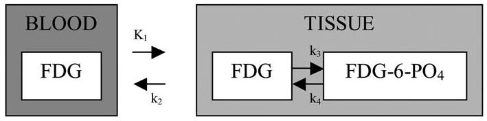
The compartmental model of Phelps et al.(1979) for FDG in human brain tissue. It describes transfer of FDG between blood and tissue and between ordinary and phosphorylated forms. Kinetic constants are rates of transfer between compartments (indicated by arrows).

$$R_C(t)=\pi e^{-t{\alpha }_1}+(1-\pi )e^{-t{\alpha }_2}$$ (10)

where

${\alpha }_{1(2)}=(1/2)(k_2+k_3+k_4\pm \sqrt{{(k_2+k_3+k_4)}^2-4k_2{k}_4})$ and π = (k₃ + k₄ − α₂)/(α₁ − α₂). Using (9), the residence density over the study period [0, T_e] is proportional to a mixture of exponentials. Thus the two-compartment model approximates the residence density of the radiotracer by a mixture of exponential densities

$$h_C(t)={\lambda }_1{e}^{-t{\alpha }_1}+{\lambda }_2{e}^{-t{\alpha }_2}$$ (11)

where (λ₁, λ₂) = (π/α₁, (1 − π)/α₂). Note that due to the time-constants, the residence density function is nonlinear in the coefficients. Thus nonlinear optimization techniques are required for compartmental model analysis. Issues of multiple minima are commonly encountered in practical applications of compartmental models to real datasets.

The standard residue functionals, flow, flux, etc., continue to be of primary interest with the two-compartment FDG model (Gjedde 1987). In the case of the distribution volume, it is the practice to only focus on the quickly cleared α₁-component. The distribution volume for this component is

$${\text{VD}}^1=\frac{K}{{\alpha }_1}$$

Note K/α₁ → (K/k₂ + k₃) as k₄ → 0. This latter formula is used to define the distribution volume of unphosphorylated deoxyglucose from an FDG study (Gjedde 1987). An analytic model allows for extrapolation so functionals can be computed for the period of observation [0, T_e], typically T_e = 90 min, as well as in the limit as T_e → ∞. The Phelps et al. (1979) approach to computation of glucose metabolic rates from FDG PET studies involves an extrapolation of the FDG computed residue with k₄ set to zero. The accuracy of this technique has been the subject of extensive debate in the literature and it remains unclear if valid assessments for human brain are even possible with this approach (Nelson, Dienel, Mori, Cruz, and Sokoloff 1987; Graham et al. 2002). Table 1 compares functional parameters of the two-compartment FDG model residue over a finite period of observation and the corresponding asymptotic values obtained by extrapolation with k₄ = 0. Note that all functionals, apart from flow, have a dependence on the period of observation. A numerical comparison for a specific choice of kinetic constants, corresponding to whole-brain (Graham et al. 2002) is presented in Table 2. Note, apart from flow, other quantities, including flux, mean transit time and extraction fraction clearly depend on the observation window. The estimated flux at T_e = 90 min is significantly lower than the value that would be generated by assuming no loss (k₄ = 0). This merely confirms that there is no way to objectively specify asymptotic extraction based on a finite experiment, in practice only studies with equivalent study durations can be compared.

Table 1.

Correspondence between functional parameters of the general residue function model, Equation (5), and kinetic constants in the two-compartment FDG residue model, Equation (11). Asymptotic values, as T_e → ∞, of functional parameters when k₄ = 0 are also shown.

Functional Parameter	General Residue Model (Equation 5)	Comp. Model (k4 ≠ 0)	Comp. Model (k4 = 0,Te ↑ ∞)
Flow (K) (ml·g−1 · min−1)	K	K1	K1
Extraction (ε)	R(Te)	RC(Te) = πe−Teα1 + (1 − π)e−Teα2	$\frac{k_3}{k_2+k_3}$
Flux (ml·g−1 · min−1)	KR(Te)	K1RC(Te)	$\frac{K_1{k}_3}{k_2+k_3}$
Median Transit Time ( ${\mu }_T^{[1/2]}$)(min)	${\mu }_T^{[0.5]}=R^{-1}(1/2)$	${\mu }_T^{[0.5]}=R_C^{-1}(1/2)$	$\frac{log(2)}{k_2+k_3}$
Distribution Volume (VDF) (ml·g−1)	$K\frac{R^{-1}(1/4)}{log(4/3)}$	$K_1\frac{R_C^{-1}(1/4)}{log(4/3)}$	$\frac{K_1}{k_2+k_3}$

Table 2.

Functional parameters corresponding to the two-compartment FDG residue model with normal brain values kinetic constants (K₁ = 0.121, k₂ = 0.172, k₃ = 0.125, k₄ = 0.0089—from Graham et al. 2002). Observable values for a T_e = 90 min study period and hypothetical (k₄ = 0) extrapolated (T_e = ∞) values are shown. The latter are obtained from the last column of Table 1.

Functional Parameter	Te = 90	Te ↑ ∞, k4 = 0
Flux (ml · g−1 · min−1)	0.034	0.051
Flux (K) (ml · g−1 · min−1)	0.121	0.121
Distribution Volume ( ${\text{V}}_D^F$) (ml · g−1)	0.530	0.407
Median Transit Time ( ${\mu }_T^{[0.5]}$)(min)	3.29	2.33
Extraction (ε)	0.28	0.42

3. Inference for the Residue Function

PET measurements of the tissue time-course C_T(t) and the arterial plasma concentration C_P(t) provide an opportunity to estimate and test hypotheses related to residues. Given the structure of the residue function, it is appropriate to regard this as a survival analysis problem involving incomplete data. Perhaps the famous survival analysis work of Kaplan and Meier (1958) was in part influenced by Meier's earlier work on residue functions for indicator dilution experiments. Indeed, although the issue of deconvolution is certainly highlighted in Equation (9), isotope decay with PET radiotracers introduces a complexity for residue analysis mirroring issues associated with covariate adjustment for survival function estimation under competing risks, see, for example, Cox and Oakes (1984). Our approach to residue estimation focuses on extraction of the conditional residence time density (h) over the interval [0, T_e] together with the blood volume (V_B), flow (K), extraction (ε), and delay (Δ). The deconvolution algorithm for estimation of the residue function is discussed first. Sampling variation is obtained by simulation. An appropriate nonparametric testing procedure for evaluation of a specified residue function model is also briefly outlined.

3.1 Deconvolution Algorithm

Techniques for the estimation of probability density functions have been well studied in the literature (Rao 1983; Silverman 1986; Wahba 1990). The simplest and most widely used approach is the histogram. The method used here is somewhat analogous. It is a cubic B-spline approximation with the number and location of knots specified to match the sampling used for measurements of the tissue time-course. B-splines have a strong pedigree in approximation theory (De Boor 1978) and of course in statistical function estimation (Stone 1994). We emphasize that this article makes no claim for the ‘optimality’ of B-spline estimators. We note that even in the context of substantially more mature nonparametric function estimation problems (e.g., density estimation), whereas B-spline estimators have a well-documented pedigree, a variety of other approaches are also viable (kernel methods, mixtures etc.). Our use of B-splines in the current setting is partially motivated by the work of Mendelsohn and Rice (1982) who found them to be effective in the context of a density deconvolution problem arising in microfluorometry. Even though our experience is that the B-spline approach is satisfactory, more sophisticated approaches might also be considered. In this regard, a general compartmental modeling approach based on approximation of residues by sums of exponentials was proposed by Cunningham and Jones (1993), see also Murase (2003). These techniques, known as spectral analysis in the PET literature, approximate the residence density using a mixture of exponentials

$$h(t)\approx {\lambda }_1{e}^{-t{\alpha }_1}+{\lambda }_2{e}^{-t{\alpha }_2}+\cdots +{\lambda }_p{e}^{-t{\alpha }_p}$$ (12)

The method of Cunningham and Jones (1993) and a number of subsequent developments have entailed prespecification of a large set of time-constants (α₁, α₂, …, α_p) so that simple nonnegative least squares computation can be applied—see also Gunn, Gunn, Turkheimer, Aston, and Cunningham (2002). A more complex computational problem arises if the time constants are included in the optimization. In any event the fundamental structure of these spectral approximations is limited by the lack of flexibility to represent residence densities that are not monotone decreasing. In particular lognormal or gamma structured densities, which have been proposed to represent observed flow distributions in capillary networks (King et al. 1996 and Ostergaard et al. 1996), cannot be approximated even by the inclusion of an infinite number of terms in Equation (12). Unlike the exponential approximations associated with compartmental models, B-spline elements generally have the flexibility to adapt to monotone (even exponential) and nonmonotone forms for the residence density. Figure 2 shows an illustration of the B-spline basis elements corresponding to a standard FDG image acquisition protocol (explained in the next section). The least squares approximation of a mixture of exponentials and a gamma density with this B-spline based are shown. Both are remarkably good.

Figure 2.

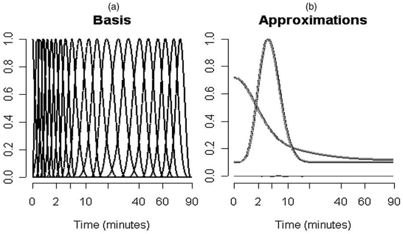
(a) B-spline basis elements for an FDG study over 90 min, (b) B-spline approximation of an exponential mixture and gamma densities. Square-root time-scales are used to better highlight the structure at early times.

With noisy data there is a trade-off between the flexibility and stability of any approximation process—the bias-variance trade-off. Thus even though Figure 2 shows that the B-spline approach has flexibility, its overall performance may be compromised by excess variability. Indeed if the real residence density conformed to a compartmental model, approximation by a more elaborate process such as B-splines might not be desirable. A practical advantage of the B-spline approach is computational—we are lead to a straightforward quadratic programming problem—which as we have indicated previously is also the case for some implementations of spectral analysis.

3.1.1 B-spline Approximation of the Residence Time Density

The tissue time-course is sampled over time-bins [t_b, t̄_b] ⊂ [0, T_e] for b = 1, 2,…, N_b. Usually the time-bins are adjoining, t̄_b = ṯ_b+1 and ṯ₁ = 0 and t̄_Nb = T_e. We employ a natural cubic B-spline basis with internal knots at the distinct values of t_b and t̄_b lying between 0 and T_e. Suppose there are a full a set of J + 3 B-splines resulting from this. The first three elements have support on the left-most time bin and provide the ability to capture the monotonic decreasing structure corresponding to residence time densities of standard one- or two-compartmental models (Murase 2003). As there is not a compelling reason to retain the corresponding basis elements on the right side, they are not included. Thus we focus on the remaining set of J basis elements. Figure 2 shows an example set of B-spline basis elements.

The J B-spline elements are denoted {B_j(·), j = 1, 2,…, J} and the approximation of the residence density is

$$h(t)=\sum _{j=1}^J{\beta }_j{B}_j(t)$$ (13)

To ensure that h is a density, it is required that β_j ≥ 0 and ${\sum }_{j=1}^J{\beta }_j{\overline{B}}_j=1$ with ${\overline{B}}_j={\int }_o^{T_e}{B}_j(t)dt$.

3.1.2 PET Data and Residue Model Discretization

Suppose the delay parameter is provisionally fixed at Δ. The PET data for the tissue region is given by z_b for b = 1, 2,…, N_b, where z_b is the total activity recorded over the bth time-bin of PET scanning

$$z_b={\int }_{{\underset{\_}{\text{t}}}_b}^{{\overline{t}}_b}{e}^{-\gamma t}{C}_T(t)dt+w_b^{-(1/2)}{\epsilon }_b$$ (14)

where ε_b represents the stochastic deviation of the measurement from that predicted by the residue model and w_b is the relative accuracy of the measurement (more on this later). Note we have introduced isotope decay via the e^−γt term in the integrand. Here γ = log(2)/τ_(1/2) where τ_(1/2) is the isotope half-life. Using the B-spline representation for the residence density the residue model can be expressed in the form of a linear regression

$$\begin{array}{l}{z}_b={\theta }_1{X}_{b1}+{\theta }_2{X}_{b2}+{\theta }_3{X}_{b3}+\dots +{\theta }_{J+2}{X}_{b(J+2)}+w_b^{-(1/2)}{\epsilon }_b\\ =X_b\theta +w_b^{-(1/2)}{\epsilon }_b\end{array}$$ (15)

where $X_{b1}={\int }_{{\underset{\_}{t}}_b}^{{\overline{t}}_b}{e}^{-\gamma t}{C}_P(t-\Delta )dt,X_{b2}={\int }_{t_b}^{{\overline{t}}_b}{e}^{-\gamma t}{\int }_o^t{C}_P(s-\Delta )dsdt$, and

$$X_{b(j+2)}=-{\int }_{t_b}^{{\overline{t}}_b}{e}^{-\gamma t}{\int }_o^{t}Bj(t-s)C_P(s-\Delta )dsdt$$

for j = 1, 2,…, J. Note the first two terms in this equation are the basis of the famous Patlak plot (Patlak, Blasberg, and Fenstermacher 1983). The θ-parameters are as follows

$$\begin{array}{cccccc}{\theta }_1=V_B,& {\theta }_2=K& \text{and}& {\theta }_{j+2}=K\zeta {\beta }_j& \text{for}& j=1,2,\dots ,J.\end{array}$$

Obviously θ_j ≥ 0 for j = 1, 2,…, J + 2. Because ζ ≤ 1 we must also have the linear inequality

$${\theta }_2-\sum _{j=1}^J{\theta }_{j+2}{\overline{B}}_j=K(1-\zeta )\ge 0$$ (16)

An upper bound on the extraction ε = (1 − ζ) can be imposed and this would certainly be appropriate in many cases. To achieve ε < ε̄, we need ${\theta }_2-{\sum }_{j=1}^J{\theta }_{j+2}{\overline{B}}_j\le K\overline{\epsilon }\equiv \overline{\epsilon }{\theta }_2$, and this yields the additional linear constraint

$$(1-\overline{\epsilon }){\theta }_2-\sum _{j=1}^J{\theta }_{j+2}{\overline{B}}_j\le 0$$ (17)

that must be satisfied. Reconstructed PET data have an approximate Poisson structure; the variance is approximately proportional to the mean (Carson et al. 1993; Maitra and O'Sullivan 1998). This structure could be incorporated into the estimation technique for θ by letting w_b = 1/(X_bθ), but our experience is that the resulting efficiency gains are of little practical significance (see also O'Sullivan and Roy Choudhury 2001). A simple weighted least squares approach with weights, w_b, inversely proportional to the observed counts, seems quite effective. Similar weighting schemes are commonly used in kinetic analysis of PET data (Huang and Phelps 1986; Mazoyer et al. 1986).

3.1.3 Regularized Estimation of B-spline Coefficients

The estimation of B-spline coefficients is based on minimization of a regularization criterion composed of the weighted residual sum of squares deviation from the model and a measure of the roughness of the target residence density. To facilitate the recovery of residence densities that undergo rapid initial variation (such as exponentials), a weighted roughness measure, with weight function, ω(t), inversely proportional to the temporal sampling density, is employed. This approach has been found effective in other settings also—e.g., O'Sullivan and Wahba (1985). The overall criterion for estimation of θ is given by

$$l_{\lambda }(\theta )=\sum _{b=1}^{N_b}{w}_b{[z_b-X_b\theta ]}^2+\lambda {\int }_0^{T_e}{[{\ddot{h}}_{\theta }(t)]}^2\omega (t)dt$$ (18)

where ḧ_θ(t) = (d²/dt²)h_θ(t) and λ > 0 is a regularization parameter. Larger values of this parameter will result in smoother solutions. The preceding formula emphasizes the dependence of the residence density on θ (see the definition in terms of β previously) but it should be appreciated that the regularization parameter accounts for scaling associated with the transformation from β to θ. Using Equation (10) the regularization criterion is expressed as a simple quadratic in θ

$$l_{\lambda }(\theta )=\sum _{b=1}^{N_b}{w}_b{[z_b-X_b\theta ]}^2+\lambda {\theta }^{\prime }\Sigma \theta$$ (19)

where Σ is a (J + 2) × (J + 2) matrix with nonzero entries ${\Sigma }_{(j+2)(k+2)}={\int }_0^{T_e}{\ddot{B}}_j(t){\ddot{B}}_k(t)\omega (t)dt$ for j, k = 1, 2,…, J. Using standard quadratic programming (QP) software (Gill, Murray, Saunders, and Wright 1986), the value of θ, which minimizes the regularization criterion subject to positivity and the linear inequality constraints in (16) and (17), can be computed. This results in an estimate θ̂_λ. Unlike compartmental residue analysis, which leads to consideration of nonlinear model forms and associated difficulties with multiple minima, the QP solution is uniquely defined. Generalized cross-validation (Wahba 1990) is used to select the regularization parameter. The criterion used here is

$$\text{GCV}(\lambda )=\frac{{\sum }_{b=1}^{N_b}{w}_b[z_b-X_b{\widehat{\theta }}_{\lambda }{]}^2}{[1-{\alpha }_{\lambda }\frac{df(\lambda )}{N_b}{]}^2}$$

where df(λ) = trace[[X′WX + λΣ]⁻¹ X′WX] with $X^{\prime }WX={\sum }_{b=1}^{N_b}{X}_b{w}_b{X^{\prime }}_b$ and α_λ is the proportion of constraints that are inactive in the solution θ̂_λ. The GCV function is minimized by grid-search over the set of (J + 1) λ-values for which df(λ_l) = l, for l = 2, 3,…, J + 2. This yields a solution θ̂ = θ̂_λ̂. The optimization over alternative delay values is done by grid-search. The optimal delay, Δ̂, is selected as the value for which the weighted residual sum of squares deviation from the data, $W\text{RSS}(\widehat{\theta })={\sum }_{b=1}^{N_b}{w}_b[z_b-X_b\widehat{\theta }{]}^2$, is minimal.

3.2 Assessment of Sampling Variation

As the estimation process involves constraints, Monte-Carlo simulation is a practical way to obtain approximations to sampling distributions. Using the pseudo-Poisson structure of PET region of interest data (Carson et al.1993), we simulate according to

$$z_b^{\ast }=X_b\widehat{\theta }+\frac{\widehat{\sigma }}{\sqrt{{\widehat{w}}_b}}{\epsilon }_b^{\ast }$$ (20)

where σ̂ is the median absolute deviation estimate of the scale of the weighted residuals $r_b=\sqrt{{\widehat{w}}_b}\cdot [z_b-X_b\widehat{\theta }]$, with weights ŵ_bi = (1/X_iθ̂), for b = 1, 2,…, N_b and ${\epsilon }_b^{\ast }$ are independent and identically distributed N(0, σ̂). Each simulated dataset yields a new estimate of θ, say θ*. Because the QP procedure used in estimation is numerically efficient, sufficient samples of θ* can be readily generated. The statistical variation in estimates of the residue or the residence distribution are constructed from the set of θ*. In particular, the sampling distribution approximations of estimates of blood volume (V_B), flow (K), mean transit time (μ_T), and flux (Kε) are readily constructed. The simulation could alternatively apply a bootstrapping procedure (drawing ${\epsilon }_b^{\ast }$ from the set of model residuals or perhaps even after the proposal of Haynor and Woods 1989), however, given that the Gaussian approximation is well supported, it is more efficient to use Gaussian deviates as a basis for the sampling.

3.3 Testing the Adequacy of a Compartment Model

There is a substantial statistical literature on nonparametric tests of this type. In the smoothing spline context see, for example, Cox, Koh, Wahba, and Yandell (1988), Hart (1997); Wahba (1990). Several authors have proposed considering the improvement in fit of the nonparametric fit relative to the fit of a null parametric model. In the present setting this test statistic becomes

$${\text{ess}}_o=\frac{W{\text{RSS}}_C-W{\text{RSS}}_N}{W{\text{RSS}}_N}$$ (21)

where W RSS_C and W RSS_N are the weighted residual sum of squares of the compartmental and nonparametric residue function estimators. The study of Liu and Wang (2004) reports very good power characteristics for tests based on (8) in the nonparametric setting. Following Xiang and Wahba (1995) the reference distribution for the test statistics is generated by simulation: Synthetic compartmental model data are simulated under the null hypothesis according to

$$z_b^{\ast }={\widehat{z}}_b+\frac{\widehat{\sigma }}{\sqrt{{\widehat{w}}_b}}{\epsilon }_b^{\ast }$$

where ẑ_b are the compartmental model predictions, σ̂ is the median absolute deviation estimate of the scale of the weighted residuals $r_b=\sqrt{{\widehat{w}}_b}\cdot [z_b-{\widehat{z}}_b]$, with weights ŵ_b = 1/ẑ_b, for b = 1, 2,…, N_B and ${\epsilon }_b^{\ast }$ are iid N(0, σ̂). Each simulated dataset, $z_b^{\ast }$ for b = 1, 2,…, N_B, is analyzed using the compartmental and B-spline approximations to obtain a value for the relative improvement in fit, ESS, associated with nonparametric residue analysis. The empirical distribution of these ESS values over a set of, say K, realizations provides an approximation to the distribution of the relative improvement in fit under the null hypothesis. Thus the p-value for the test of hypothesis is approximated as the fraction of times ESS is greater than or equal to ess_o in these K simulations. Hence

$$P[\text{ESS}\ge {\text{ess}}_o]=p–\text{value}\approx \frac{\#[\text{ESS}\ge {\text{ess}}_o]}{K}$$ (22)

By choice of K, the accuracy of the preceding p-value calculation can be controlled. In our experience K = 1,000 appears to be sufficient.

In the application to the FDG datasets this analysis is applied to a collection of separate datasets, corresponding to different subjects and to data from separated regions within the same subject. The overall evaluation of the hypothesized model structure requires analysis of the collection of p-values computed over the individual datasets. Note that under the null hypothesis, the distribution of p-values should be uniform. Thus comparing the distribution of p-values to the uniform provides an assessment of the combined hypothesis. The standard Kolmogorov-Smirnov test (Conover 1971) is used for this assessment.

4. Application and Results

¹⁸F-Fluorodeoxyglucose (Phelps et al. 1979, Spence et al. 1998) is the most widely used PET radiotracer. It is used to assess glucose utilization characteristics of tissues in vivo. Graham et al. (2002) reported on a series of PET studies with ¹¹C-glucose and FDG in 12 normal subjects. Here we analyze the FDG component of these data using the nonparametric residue analysis. We also undertake a statistical evaluation of the adequacy of the two-compartment FDG model for these data.

4.1 Normal Cerebral PET FDG Data

FDG was injected intravenously followed by PET imaging of the time-course of the radiotracer in the brain using a GE Advance scanner. Dynamic time-binned volumetric images of the radioactivity (measured in counts) were acquired over a 90 min time period (T_e). A total of 31 time-binned scans were acquired and were reconstructed with attenuation correction and a Hanning filter to obtain images with a resolution of approximately 6 mm full width at half maximum. The temporal sampling frequency varied throughout the 90 min, with more intensive sampling occurring immediately after the tracer injection. The sampling protocol entailed a 1 min preinjection scan followed by four (15-sec) scans, four (30-sec) scans, four (1-min) scans, four (3-min) scans and 14 (5-min) scans. Each scan provided a time-binned image volume with a total N = 128 × 128 × 35 voxels arranged as transverse slices throughout the brain—35 (4.5 mm thick) planes with 128 × 128 (2.3 mm × 2.3 mm) pixels per plane. Regions of interest (ROI) corresponding to eight structures within the grey matter (thalamus, caudate, parietal, frontal lobe, putamen, temporal lobe, cerebellum, and occipital cortex) as well as a white matter and whole brain regions were identified using coregistered MR scans. Thus a total of 10 ROIs for a set of 12 normal subjects were available for analysis. Excluding whole brain, which is around 5,000 voxels, the regions range from 150–1,000 voxels with a typical size of 650 voxels. Blood sampling was carried out using an automated blood sampler connected to an arterial catheter inserted into the radial artery. One-milliliter samples were obtained at 20-s intervals initially, followed by progressively longer intervals. Additional details of the data are reported in Graham et al. (2002).

4.2 An Illustration

Figure 3 shows the results of application of the standard two-compartment model and the nonparametric residue to PET FDG time-course data from a cerebellum ROI in a normal subject. On the uptake scale, differences between the fits are imperceptible, but a deeper statistical analysis is of interest. The standardized weighted residuals

Figure 3.

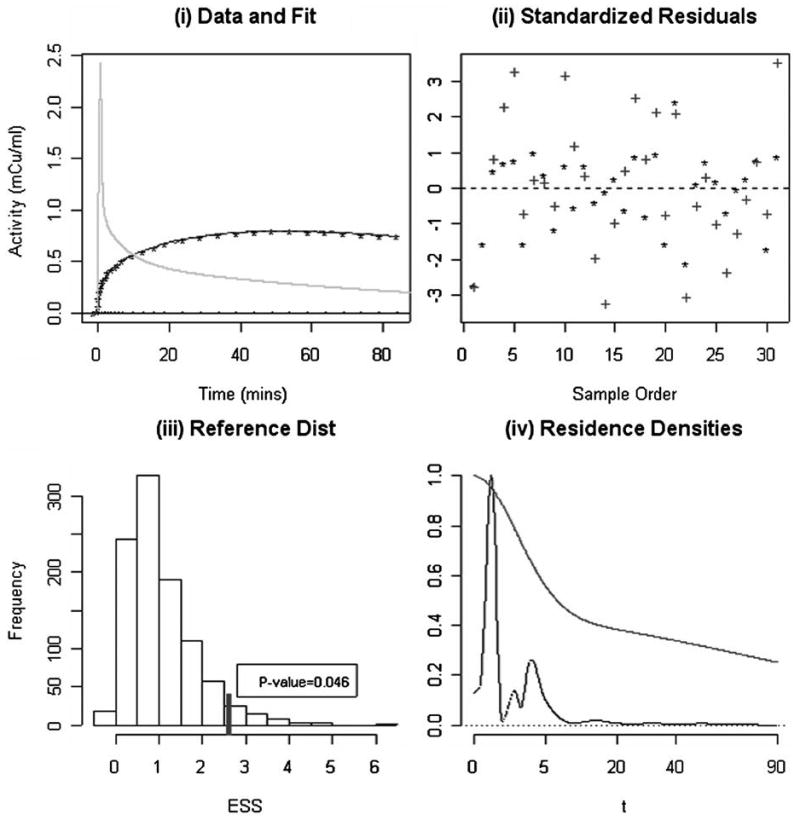
(i) The observed PET time course data (*) for a Cerebellum ROI and fits obtained with the nonparametric and 2-compartment approximations of the residence density (lines); the spiked curve is the arterial blood input function (C_p). (ii) Standardized weighted residuals corresponding to the fits in (i) for the residue (*) and compartmental (+) analysis. (iii) Reference distribution for the relative improvement in fit statistic, obtained by simulation. The observed improvement in fit is 2.73 (marked) and the empirical p-value (0.046) is indicated. (iv) Nonparametric and compartment (smoother curve) model estimates of the tissue residence density of F-18 label. Both densities are scaled to maximum of unity.

$$r_i=\frac{\sqrt{{\widehat{w}}_i}\cdot [z(t_i)-\widehat{z}(t_i)]}{\widehat{\sigma }},$$

where ẑ(t_i) is the fitted time-course and σ̂ is defined as the median absolute deviation (for the nonparametric analysis), are shown in Figure 3(b). Here we see that the compartment model residuals are generally larger in magnitude. The relative improvement in fit, ess_o, is 2.73. Using simulation with K = 1,000 realizations, the reference distribution calculation shows that the expected improvement in fit associated with nonparametric residue analysis is 0.87. The observed value of 2.73 is in the extreme of the computed reference distribution, Figure 3(c). Thus there is strong statistical evidence against the hypothesis that the compartment model is consistent with this dataset, the p-value is 0.046. The nonparametric residue analysis suggests a distinctly nonmonotone pattern in residence time density, see Figure 3(d). A comparison between functional parameters obtained from the compartmental and nonparametric residue analysis is provided in Table 3. The reported standard errors were obtained by simulation. Table 3 shows some differences for volume of distribution and blood volume but discrepancies for flow, flux, mean transit time, and extraction are minor.

Table 3.

Estimated functionals (± standard errors) of the tissue residue for parametric compartmental and nonparametric residue analysis of the PET data (corresponding to a frontal lobe ROI) in Figure 3. Functionals are defined in Table 1. Standard errors are estimates by simulation—see text.

Residue	Flow K	Blood Volume VB	Distribution Volume ${\text{V}}_D^F$	Flux Kε	Transit Time ${\mu }_T^{[0.5]}$	Extraction ε
Compartmental	0.119 ± 0.012	0.022 ± 0.021	0.584 ± 0.063	0.030 ± 0.001	3.70 ± 1.08	0.252 ± 0.021
Nonparametric	0.118 ± 0.013	0.039 ± 0.025	0.441 ± 0.113	0.033 ± 0.001	3.61 ± 1.32	0.277 ± 0.028

4.3 Statistical Analysis of 120 ROI Time-Course Data Sets

The collection of ROI time course datasets have each been analyzed by a procedure identical to that used in the preceding illustration. Figure 4 shows the distributions of p-values obtained by brain region and overall. Brain ROIs show the strongest evidence against the two-compartment model. This is perhaps not so surprising because these ROIs are relatively large and possibly heterogenous. With the exception of the caudate, within each brain region the overall plausibility of the two-compartment model is rejected at the 0.001 level by the Kolmogorov-Smirnov test. The distribution of p-values, with brain ROIs eliminated, is shown in Figure 4(b). The distribution of p-values shows substantial lack of agreement with a uniform distribution, pointing to a systematic difficulty of the two-compartment model to adequately represent PET FDG time course data from normal brain regions. The overall p-value obtained by applying the Kolmogorov-Smirnov test to data from all subjects and regions (without the brain) is well below 0.0001. Inclusion of the brain region data further reduces this p-value.

Figure 4.

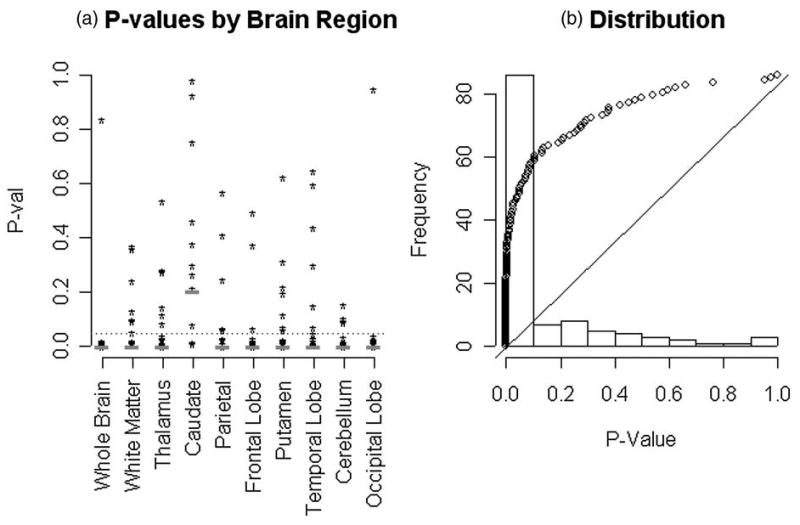
(a) Individual p-values evaluating the fit of the two-compartment model, for each of the 120 datasets analyzed (10 regions for 12 normal subjects). Individual brain regions are indicated. The p-values of the Kolmogorov-Smirnov test across subjects are indicated with the red dash. The dotted blue line shows the 0.05 significance level. (b) Distribution of p-values and a quantile-quantile comparison with the uniform distribution (the 12 whole brain ROIs are not included here, the result is more extreme with them included). The relevant Kolmogorov-Smirnov test has a p-value ≪0.0001.

It should be noted that the 10 brain regions within each subject are well-separated and it is unlikely that the reconstruction process would induce significant auto-correlation between PET measurements from different regions within the same subject (c.f. Maitra and O'Sullivan 1998). In addition the test statistic used is based on the extrasums of squares, which could reasonably be expected to remove further sources of regional correlation related to the biology. For example the extrasums of squares used is invariant to the scale of the data. Even if there existed significant correlations between the test-statistic values in distinct brain regions, under the null hypothesis the distribution of p-values across subjects within a given brain regions should be uniform. Figure 4(a) shows that apart from the caudate there is substantial lack of conformity to the uniform. The Kolmogorov-Smirnov tests confirm this. Bonferroni adjustment of the p-values for multiple comparisons across regions still finds overwhelming evidence against the two-compartment model in all but the caudate region.

Table 4 presents statistical summaries, means, and standard deviations over the 12 subjects, of functional parameters resulting from two-compartmental and nonparametric residue analyses. The regional mean values produced by either technique are generally in agreement with each other and well within ranges of variation that have appeared in the literature—see, for example, the review in Graham et al. (2002). A summary of the average percent differences between regional means and standard deviations produced by the two-compartmental and nonparametric residue analyses is presented in Table 5. Note this table is produced by summarizing the regional values in Table 4. The results show a number of small but statistically significant differences between averages of regional mean values from compartmental and nonparametric residue analysis. The smallest difference is for flux (4% larger with nonparametric residue analysis) and the largest difference is for flow (26% greater with the nonparametric residue analysis). Statistically significant increases in standard deviations of functional parameters are found. The most dramatic of these is for flow where the variability is three times greater with the nonparametric approach—although it must be noted that the uncertainty in this estimate is also substantial.

Table 4.

Mean ± SD of functional parameters for the FDG tissue residue (90 min study duration). Statistics are for 10 normal human subjects (raw data are plotted in Figure 4). Different brain regions are indicated. Values obtained from the two-compartment model analysis (c.f. Table 1 and 2) are shown above corresponding values produced by the nonparametric residue analysis.

Region	Flow K	Blood Volume VB	Distribution Volume ${\text{V}}_D^F$	Flux Kε	Transit ${\mu }_T^{[0.5]}$	Extraction ε
							Whole	0.108 ± 0.026	0.038 ± 0.034	0.500 ± 0.079	0.032 ± 0.007	3.79 ± 1.35	0.306 ± 0.066
Brain	0.137 ± 0.053	0.042 ± 0.036	0.427 ± 0.248	0.033 ± 0.006	2.37 ± 2.01	0.269 ± 0.088
White	0.077 ± 0.021	0.029 ± 0.022	0.449 ± 0.073	0.023 ± 0.007	4.75 ± 1.43	0.308 ± 0.073
Matter	0.091 ± 0.031	0.027 ± 0.019	0.363 ± 0.151	0.024 ± 0.007	2.92 ± 1.72	0.277 ± 0.066
Thalamus	0.125 ± 0.028	0.053 ± 0.036	0.530 ± 0.140	0.033 ± 0.008	3.41 ± 1.25	0.270 ± 0.061
	0.160 ± 0.083	0.054 ± 0.057	0.484 ± 0.241	0.034 ± 0.007	2.95 ± 2.73	0.255 ± 0.108
Caudate	0.121 ± 0.034	0.040 ± 0.030	0.507 ± 0.144	0.037 ± 0.008	3.82 ± 2.24	0.330 ± 0.108
	0.107 ± 0.021	0.054 ± 0.028	0.598 ± 0.241	0.039 ± 0.008	4.16 ± 1.88	0.366 ± 0.065
Parietal	0.117 ± 0.024	0.052 ± 0.039	0.550 ± 0.100	0.035 ± 0.006	3.80 ± 1.38	0.308 ± 0.055
Lobe	0.151 ± 0.108	0.056 ± 0.044	0.492 ± 0.190	0.037 ± 0.006	3.10 ± 1.83	0.301 ± 0.111
Frontal	0.112 ± 0.024	0.047 ± 0.034	0.552 ± 0.070	0.036 ± 0.008	4.17 ± 1.49	0.334 ± 0.075
Lobe	0.176 ± 0.078	0.028 ± 0.027	0.385 ± 0.181	0.038 ± 0.008	2.02 ± 1.88	0.253 ± 0.117
Putamen	0.128 ± 0.022	0.047 ± 0.028	0.540 ± 0.136	0.039 ± 0.008	3.30 ± 0.99	0.308 ± 0.061
	0.180 ± 0.130	0.051 ± 0.049	0.533 ± 0.225	0.040 ± 0.007	3.44 ± 2.78	0.292 ± 0.129
Temporal	0.103 ± 0.022	0.046 ± 0.032	0.557 ± 0.096	0.031 ± 0.006	4.28 ± 1.21	0.310 ± 0.066
Lobe	0.116 ± 0.038	0.052 ± 0.046	0.498 ± 0.278	0.032 ± 0.005	3.44 ± 2.22	0.300 ± 0.095
Cerebellum	0.147 ± 0.037	0.033 ± 0.031	0.530 ± 0.071	0.024 ± 0.005	2.77 ± 0.76	0.172 ± 0.051
	0.158 ± 0.081	0.055 ± 0.043	0.614 ± 0.300	0.025 ± 0.005	2.81 ± 1.69	0.179 ± 0.060
Occipital	0.135 ± 0.032	0.060 ± 0.043	0.584 ± 0.154	0.036 ± 0.010	3.41 ± 1.09	0.272 ± 0.059
Cortex	0.202 ± 0.144	0.058 ± 0.055	0.559 ± 0.266	0.038 ± 0.010	2.65 ± 2.21	0.245 ± 0.117

Table 5.

Mean ± SD across 12 brain regions. of percent differences between means and standard deviations (over 10 subjects) of regional functional parameter estimates computed by the compartmental and nonparametric residue analysis (i.e., columnwise summary of values in Table 4). Single or double asterisk indicate values, which show significant (at the 0.05 or 0.01 levels) deviation from zero by a simple z-test.

% Difference	Flow K	Blood Volume VB	Dist. Volume ${\text{V}}_D^F$	Flux Kε	Transit Time ${\mu }_T^{[1/2]}$	Extraction ε
Mean	26 ± 21*	9 ± 28	−7 ± 15	4 ± 1**	−18 ± 20*	−6 ± 10
SD	191 ± 163*	23 ± 32*	135 ± 84*	−4 ± 6*	72 ± 60*	49 ± 50*

Residuals obtained from the nonparametric residue and compartmental model analyses show substantial conformity to the Gaussian assumption. There are some outliers, but after trimming 3% of the most extreme values, the residual histogram is remarkably Gaussian (Figure 5(a)). This diagnostic supports the simulation model used for approximation of sampling distributions. The marginal distribution of the standardized residuals (trimmed) is also shown in Figure 5(b). Residuals are generally larger for the compartmental model analysis, which was confirmed by the more formal analysis previously.

Figure 5.

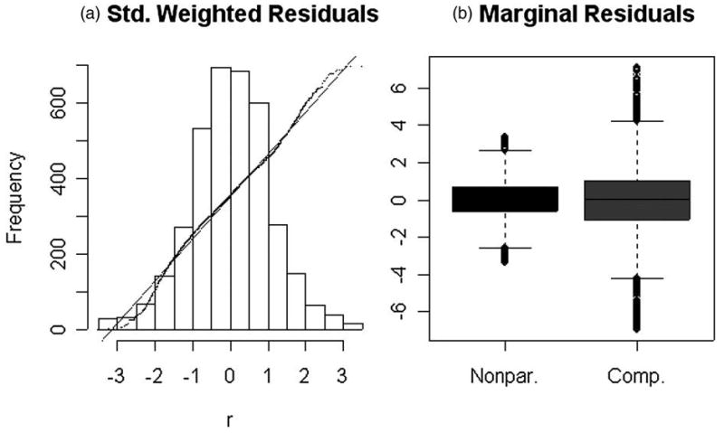
(a) Diagnostic assessment of the approximate Gaussian structure of residuals from the nonparametric residue analysis—3% of outlying values have been trimmed. Histogram and quantile-quantile comparison with a standard Gaussian are shown. (b) Marginal distribution of the nonparametric and 2–compartment model residuals—again 3% of outlying values have been trimmed.

5. Discussion

We have described an approach, based on an extension of the indicator dilution work of Meier and Zierler (1954), for the representation of radiotracer uptake data measured by PET. A new class of survival analysis problems with incomplete measurements is identified. These are called residue analysis problems. Nonparametric inference for the residue is developed. Our approach is based on consideration of the residence density associated with the residue function. The nonparametric estimation of the residence density is addressed using the method of regularization with cross-validation—an established approach to nonparametric function estimation, see Mendelsohn and Rice (1982) and Wahba (1990). Computations with B-splines lead to a quadratic programming problem with unique and readily evaluated solutions. No claim for optimality of this approach is made. Indeed, whereas the method of regularization with cross-validation has a solid theoretical basis, including a range of consistency results, a variety of other nonparametric approaches to density estimation might equally well be adapted to this problem. Salient biological functionals of the residue are described and appropriate simulation methods applied to obtain approximate standard errors and reference distributions for tests of hypotheses. The methodology is used to evaluate the degree of statistical support for the hypothesis of two-compartment model of Phelps et al. (1979) for cerebral PET-FDG applications. This is the first attempt to rigorously evaluate this model construct using in vivo measurements in humans.

Data from a series of PET FDG studies in normal brain are used. A total of 120 time-courses from 12 subjects and 10 brain regions are involved. The evidence against the established model is very strong. Whereas rigorous statistical support of this finding is novel, suspicions regarding the appropriateness of the two-compartmental model have been the subject of debate in the literature for some time. Our study does not refute the basic biochemistry of the two-compartment model, indeed this has been well validated by in-vitro test-tube experimentation. Rather the difficulty with the model arises from the realization that a typical PET region of interest need not behave as a well-stirred test-tube sample. The delivery of the PET radiotracer is clearly not a simple diffusion from a well-mixed compartment but instead arises from specific flow paths through local vasculature. The specific biochemical configuration confronted by the radiotracer cannot be considered uniform throughout the tissue region. Thus our result is most likely explained in terms of tissue heterogeneity. The brain regions considered here, similar to those in many PET studies, are relatively large—ranging from several hundred to several thousand cubic centimeters in volume. Within such regions it is likely that neither the vascular delivery characteristics nor local biochemistry will be homogeneous. Thus the expected response obtained from these regions would not behave as a simple compartmental model. This is a point made in a very convincing fashion by Lucignani et al. (1993) and in the earlier work of Nelson et al. (1987). Even with voxel-level PET data, whose nominal resolution for human brain studies is currently on the order of 0.25 cm³, the assumption of homogeneity is still difficult to justify (O'Sullivan 1993, 2006). In view of this it is hardly surprising that the two-compartmental model would not accurately represent the local residue of FDG in tissue.

Partial volume (PV) correction has not been applied to our ROI time course data and there might be some concern that inhomogeneities introduced by PV artifacts play a role here. This explanation seems unlikely. Given the ROI sizes and the scanner resolution, the case for consideration of such PV corrections is not compelling. The ROIs range from 150–1000 voxels with a typical size of 650 voxels. This is excluding the whole brain, which is around 5,000 voxels. The resolution full-width at half maximum (FWHM) of the PET scanner used is approximately 6.5 mm (3 pixels) within plane and 1-pixel between planes. In this range it is unlikely that PV artifacts significantly contribute to ROI averages—see Figure 3 of Rousset, Ma, and Evans (1998). The ROI, which might be considered the most influenced by potential PV artifacts, is the caudate. This is the smallest ROI considered in our study. It is notable that it is only in this region that there is a failure to reject the FDG two-compartment model hypothesis. Because the PV artifact does not lead to model rejection in the smallest ROI, it is unlikely that this issue that plays a much smaller role in larger ROIs could explain our results. It is also important to appreciate that the impact of PV on time course patterns is known to be pronounced in the case of isolated ‘hot’ or ‘cold’ ROIs in a cold or hot bath. This is certainly not the configuration in which the brain regions in our study present. The dominant impact of PVadjustment is potential removal (deconvolution) of the effect of the resolution filter. As our resolution filter is time-invariant, the primary impact of PV would be to influence scale but not the shape of the time-courses analyzed. In particular it is difficult to imagine that PV effects would convert an exponential residence pattern into one that no-longer peaks at zero. Furthermore the relatively long acquisition time used in this study is perhaps a more important source of concern—subjects are conscious and artifacts associated with their not being able to keep their heads perfectly still for the duration of these studies are likely to also be present. Artifacts generated by such movements are maybe of somewhat greater significance than PV—they may also impact attenuation correction. But again the situation with the caudate ROI, which would also be most affected by such artifacts, require that we look in a different direction to develop a likely explanation for our results. On the other hand failure to reject on the smallest (and therefore the most homogeneous) ROI is consistent with the hypothesis that the explanation lies in tissue heterogeneity. Thus tissue heterogeneity remains our working hypothesis.

The pattern of departures from the compartmental model is clarified by pooling across subjects. The statistical arguments underlying the definition of residue imply that the residue function resulting from pooling J separate tissue regions is the flow-weighted average of the individual residue functions

$$\begin{array}{l}\overline{R}(t)=\frac{K_1{R}_1(t)+K_2{R}_2(t)+\dots +K_J{R}_J(t)}{K_1+K_2+\dots +K_J}\\ ={\omega }_1{R}_1(t)+{\omega }_2{R}_2(t)+\dots +{\omega }_J{R}_J(t)\end{array}$$ (23)

where ω_j = K_j/(K₁ + K₂ + … + K_J) for j = 1,2, …, J is the fractional flow through the j′^th tissue. Writing $\overline{R}(t)=1-\overline{\zeta }{\int }_o^t\overline{h}(\tau )d\tau$, the pooled residence time density, h̄, is also a weighted average but in this case the weighting is modified by exchange ratios, ζ_j = (1 − ε_j). The pooled residence density is

$$\begin{array}{l}\overline{h}(t)=\frac{K_1{\zeta }_1{h}_1(t)+K_2{\zeta }_2{h}_2(t)+\dots +K_J{\zeta }_J{h}_J(t)}{K_1{\zeta }_1+K_2{\zeta }_2+\dots +K_J{\zeta }_J}\\ ={\pi }_1{h}_1(t)+{\pi }_2{h}_2(t)+\dots +{\pi }_J{h}_J(t)\end{array}$$ (24)

where π_j = K_jζ_j/(K₁ζ₁ + K₂ζ₂ + … + K_Jζ_J) for j = 1,2, …, J. Figures 6 and 7 present regional means of residues and residence densities obtained by pooling across the 12 subjects analyzed. Across all regions (apart from the caudate) there is evidence of nonmonotone residence density patterns. Comparison with an average compartment model residue (defined here by the averages of kinetic constants) is also presented in the Figures 6 and 7. Nonparametrically estimated residence time densities are clearly nonmonotone and quite consistent with lognormal type distributions that have been used to represent microvascular (flow) heterogeneities (c.f. King et al. 1996; Ostergaard et al. 1996). Figures 6 and 7 provide little support for exponentially decaying residence densities or even monotonely decreasing ones that are implied by spectral analysis (Cunningham and Jones 1993; Gunn et al. 2002; Murase 2003; Keeling et al. 2004).

Figure 6.

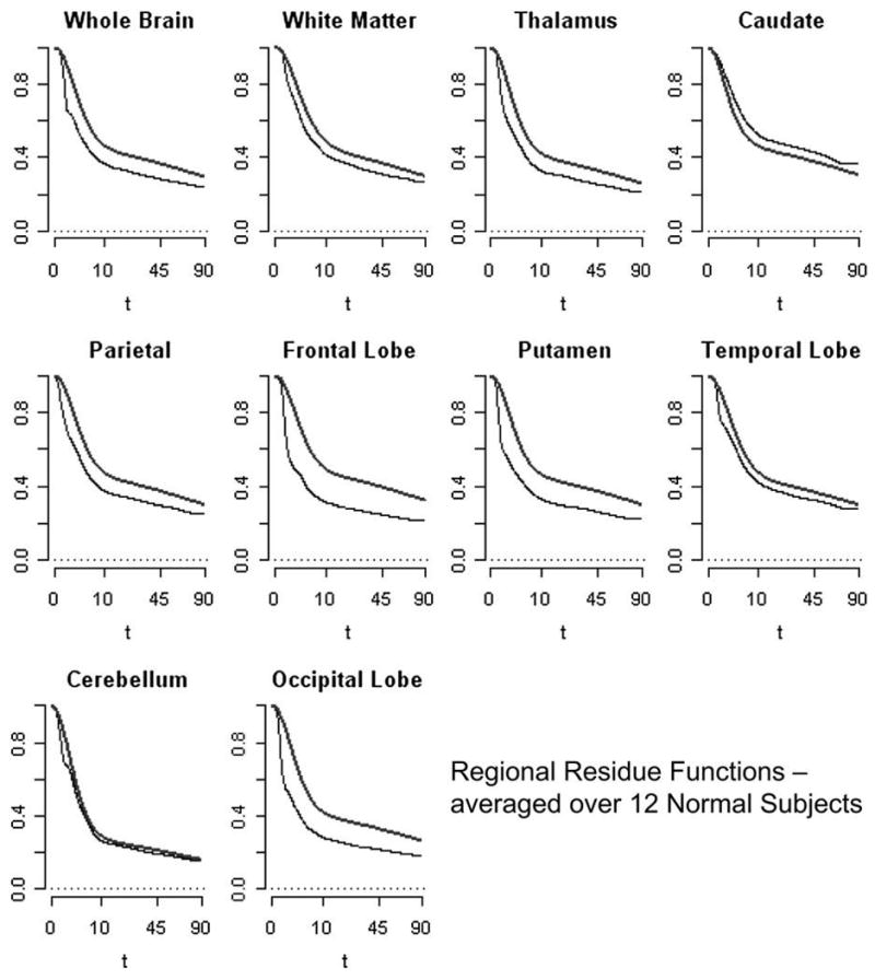
Pooled (Equation 23) residues estimated nonparametrically (lower curve) and using the average parameters for the two-compartment model (higher curve). Results for each of 10 brain regions are shown. Note the square-root time scale is used.

Figure 7.

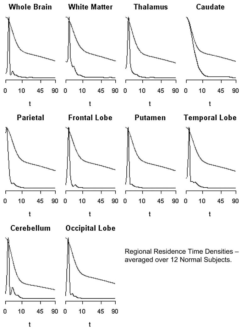
Pooled (Equation 24) residence densities estimated nonparametrically (spiked) and using the average parameters for the two-compartment model (monotone decreasing with higher tail). Results for each of 10 brain regions are shown. Note the square-root time scale and the densities are scaled to have a common maximum.

There is an extensive physiological literature on mechanisms of blood-tissue exchange in cerebral and other tissues—see Li et al. (1997) for a review. The assumption that regional cerebral tissue behaves as a well-stirred compartment is not well supported by theory or indeed by previous direct measurement. Granted, the ability to obtain convincing data in humans has been limited, but data from rat studies (Abounader, Vogel, and Kuschinsky1995; Hudetz, Biswal, Feher, and Kampine 1997) have not been supportive of a compartmental representation. Ostergaard et al. (1999) carefully review a number of previous studies and find no evidence to support the hypothesis of exponential flow patterns in brain tissue. Similar conclusions have been reported based on detailed measurements of myocardial tissues (Kroll et al. 1996). The analysis presented here shows that in vivo PET measurements have the power to address detailed questions related to structure of the tissue residue. By properly adjusting for the increased flexibility of nonparametric residue analysis, valid statistical assessments of the compartment model hypothesis have been possible. Thus we have developed in vivo human data that point to a significant physiologic inaccuracy in the use of compartmental models for quantitation of regional cerebral (FDG) glucose utilization. This inaccuracy has the greatest impact on the assessment of the flow. Our analysis might also be considered at the voxel-level but, because PET time-course data have very high variability and are spatially correlated (Carson et al. 1993; Maitra and O'Sullivan 1998), it is unlikely that there would be sufficient power to evaluate if the compartment model applies on voxel-level scales—i.e., over volumes on the order of milliliters. Nevertheless the physiological wisdom contained in Bassingthwaighte (1970) and a number of subsequent authors would argue against the compartmental construct being appropriate.

Traditionally in statistics the realization that a process does not conform to the assumptions of a specific model (Gaussian, exponential, Weibull etc.) has been a motivation for the development of nonparametric approaches to analysis. With survival time data the famous Kaplan-Meier estimator is the outstanding example. In a similar way, for data from PET radiotracer studies, nonparametric residue analysis offers a way to consider alternatives rather than just blindly applying a potentially inappropriate parametric compartmental model. Importantly the nonparametric approach is fully interpretable biologically. As developed in Section 2, the nonparametric method yields the key functionals of the residue—flux, flow, distribution volume etc. Our analysis shows that quantitation of dynamic FDG data from normal brain regions via the standard compartment model is flawed—the statistical evidence is overwhelming. Even though the flux functional is quite robust to the specification of the residue—a result which underpins the Patlak approach—there are other functionals, notably flow and transit time, that are not robust in this sense. For these quantities, analysis based on the flawed compartmental model cannot be recommended. In general a nonparametric techniques offers reduced bias with some increased variability. In the case where a parametric model is invalid and produces questionable results, it is appropriate to put more reliance in nonparametric procedures that can offer consistency.

Intermediate semiparametric approaches to residue analysis might also be considered. Blood-tissue exchange constructs (Bassingthwaighte 1970, Li et al. 1997) separate processes governing the extraction and metabolism from those associated with flow patterns. In a similar way the total residence time (T) of the label in tissue could be considered as a sum of the time spent in the vasculature (T_V) and the time undergoing extravascular transport and metabolism (T_M), i.e.

$$T=T_V+T_M$$

If we assume that T_V and T_M are independent, then the overall residence time density will be the convolution of the densities for the vascular and extravascular processes. Test-tube biochemistry might well provide parametric (even compartmental) representations for the distribution of T_M, whereas nonparametric distributions could be considered for T_V. This would lead to a semiparametric representation for the residue analysis. The literature provides a strong argument in favor of the vascular transport T_V having a nonmonotone pattern—lognormal type distribution. A compartment model for the extravascular component, T_M, would then imply an overall residence density that peaks away from zero. This is fully consistent with the patterns recorded in Figure 7. Provided the semiparametric approach is unbiased, its advantage might be improved reduced variability.

Overall this work, which is stimulated by the Meier and Zierler's survival function development of indicator dilution theory, offers a new opportunity for development of survival analysis techniques with incomplete data that should be of substantial interest to the molecular imaging community. There are a range of considerations related to multiple injection studies, recirculating metabolites, nonlinearities associated with ligand imaging etc. where innovations or adaptations of residue analysis are required. Extension of the methodology for voxel-level implementation is also of interest.

References

- Abounader R, Vogel J, Kuschinsky W. Patterns of Capillary Plasma Perfusion in Brains of Conscious Rats During Normocapnia and Hypercapnia. Circulation Research. 1995;76:120–126. doi: 10.1161/01.res.76.1.120. [DOI] [PubMed] [Google Scholar]
- Axel L. Cerebral Blood Flow Determination by Rapid-Sequence Computed Tomography: Theoretical Analysis. Radiology. 1980;137(3):679–686. doi: 10.1148/radiology.137.3.7003648. [DOI] [PubMed] [Google Scholar]
- Bassingthwaighte JB. Blood Flow and Diffusion Through Mammalian Organs. Science. 1970;167:1347–1353. doi: 10.1126/science.167.3923.1347. [DOI] [PMC free article] [PubMed] [Google Scholar]
- Carson RE, Yan Y, Daube-Witherspoon ME, Freedman N, Bacharach SL, Herscovitch P. An Approximation Formula for PET Region-of-Interest Values. IEEE Transactions on Medical Imaging. 1993;12:240–251. doi: 10.1109/42.232252. [DOI] [PubMed] [Google Scholar]
- Conover WJ. Practical Nonparametric Statistics. New York: John Wiley & Sons; 1971. [Google Scholar]
- Cox D, Koh E, Wahba G, Yandell B. Testing The (Parametric) Null Model Hypothesis In (Semiparametric) Partial And Generalized Spline Models. Ann Statist. 1988;16:113–119. [Google Scholar]
- Cox DR, Oakes D. Analysis of Survival Data. London: Chapman and Hall; 1984. [Google Scholar]
- Cunningham VJ, Gunn RN, Matthews JC. Quantification in Positron Emission Tomography for Research in Pharmacology and Drug Development. Nuclear Medicine Communications. 2004;25:643–646. doi: 10.1097/01.mnm.0000134330.38536.bc. [DOI] [PubMed] [Google Scholar]
- Cunningham VJ, Jones T. Spectral Analysis of Dynamic PET Studies. Journal of Cerebral Blood Flow and Metabolism. 1993;13:15–23. doi: 10.1038/jcbfm.1993.5. [DOI] [PubMed] [Google Scholar]
- De Boor C. A Practical Guide to Splines. New York: Springer-Verlag; 1978. [Google Scholar]
- Gill PE, Murray W, Saunders MA, Wright MH. User's Guide for LLSOL (Version 1.0), Report SOL 86-1. Department of Operations Research, Stanford University; California: 1986. [Google Scholar]
- Gjedde A. Does Deoxyglucose Uptake in the Brain Reflect Energy Metabolism. Journal de Pharmacologie. 1987;36:1853–1861. doi: 10.1016/0006-2952(87)90480-1. [DOI] [PubMed] [Google Scholar]
- Graham MM, Muzi M, Spence AM, O'Sullivan F, Lewellen TK, Limk JM, Krohn KA. The Fluorodeoxyglucose Lumped Constant in Normal Human Brain. Journal of Nuclear Medicine. 2002;43:1157–1166. [PubMed] [Google Scholar]
- Gunn RN, Gunn SR, Turkheimer FE, Aston JAD, Cunningham VJ. Positron Emission Tomography Compartmental Models: A Basis Pursuit Strategy for Kinetic Modeling. Journal of Cerebral Blood Flow and Metabolism. 2002;22:1425–1435. doi: 10.1097/01.wcb.0000045042.03034.42. [DOI] [PubMed] [Google Scholar]
- Hart JD. Nonparametric Smoothing and Lack-of-Fit Tests. New York: Springer-Verlag; 1997. [Google Scholar]
- Haynor DR, Woods SD. Resampling Estimates of Precision in Emission Tomography. IEEE Transactions on Medical Imaging. 1989;8:337–343. doi: 10.1109/42.41486. [DOI] [PubMed] [Google Scholar]
- Huang SC, Phelps ME. Principles of Tracer Kinetic Modeling in Positron Emission Tomography and Autoradiography. New York: Raven Press; 1986. [Google Scholar]
- Huang SC, Phelps ME, Hoffman EJ, Sideris K, Selin CJ, Kuhl DE. Noninvasive Determination of Local Cerebral Metabolic Rate of Glucose in Man. The American Journal of Physiology. 1980;238:E69–E82. doi: 10.1152/ajpendo.1980.238.1.E69. [DOI] [PubMed] [Google Scholar]
- Hudetz AG, Biswal BB, Feher G, Kampine JP. Effects of Hyposix and Hypercapnia on Capillary Flow Velocity in the Rat Cerebral Cortex. Microvascular Research. 1997;54:35–42. doi: 10.1006/mvre.1997.2023. [DOI] [PubMed] [Google Scholar]
- Kaplan EL, Meier P. Nonparametric Estimation From Incomplete Observations. Journal of the American Statistical Association. 1958;53:457–481. [Google Scholar]
- Keeling SL, Bammer R, Kogler T, Stollberger R. Technical Report 289. University of Graz &Graz Technical Institute; 2004. On the Convolution Model of Dynamic Contrast Enhanced Magnetic Resonance Imaging and Nonparametric Deconvolution Approaches. http://www.kfunigraz.ac.at/imawww/invcon/medimage/kernel.pdf. [Google Scholar]
- King RB, Raymond GM, Bassingthwaighte JB. Modeling Blood Flow Heterogeneity. Annals of Biomedical Engineering. 1996;24:352–372. doi: 10.1007/BF02660885. [DOI] [PMC free article] [PubMed] [Google Scholar]
- Kroll K, Wilke N, Jerosch-Herold M, Wang Y, Zhang Y, Bache RJ, Bassingthwaighte JB. Modeling Regional Myocardial Flows from Residue Functions of an Intravascular Indicator. Am J Physiol. 1996;271:H1643–H1655. doi: 10.1152/ajpheart.1996.271.4.H1643. [DOI] [PMC free article] [PubMed] [Google Scholar]
- Larson KB, Perman WH, Perlmutter JS, Gado MH, Ollinger JM, Zierler K. Tracer-Kinetic Analysis for Measuring Region Blood Flow by Dynamic Nuclear Magnetic Resonance Imaging. Journal of Theoretical Biology. 1994;170:1–14. doi: 10.1006/jtbi.1994.1164. [DOI] [PubMed] [Google Scholar]
- Li Z, Yipintsoi T, Bassingthwaigthe JB. Modeling Blood Flow Heterogeneity. Annals of Biomedical Engineering. 1997;25:604–619. doi: 10.1007/bf02684839. [DOI] [PMC free article] [PubMed] [Google Scholar]
- Liu A, Wang Y. Hypothesis Testing in Smoothing Spline Models. J Statist. Computing and Simulation. 2004;74:581–597. [Google Scholar]
- Lucignani G, Schmidt KC, Moresco RM, Striano G, Colombo F, Sokoloff L, Fazio F. Measurement of Regional Cerebral Glucose Utilization With Fluorine-18-FDG and PET in Heterogeneous Tissues: Theoretical Considerations and Practical Procedure. Journal of Nuclear Medicine. 1993;34:360–369. [PubMed] [Google Scholar]
- Maitra R, O'Sullivan F. Variability Assessment in PET and Related Generalized Deconvolution Problems. Journal of the American Statistical Association. 1998;93:1340–1356. [Google Scholar]
- Mankoff DA, Muzi M, Zaidi H. Quantitative Analysis in Nuclear Oncologic Imaging. In: Zaidi H, editor. Quantitative Analysis in Nuclear Medicine Imaging. New York: Springer; 2005. pp. 416–453. [Google Scholar]
- Mazoyer BM, Huesman RH, Budinger TF, Knittel BL. Dynamic PET Data Analysis. Journal of Computer Assisted Tomography. 1986;10:645–653. doi: 10.1097/00004728-198607000-00020. [DOI] [PubMed] [Google Scholar]
- Meier P, Zierler KL. On the Theory of the Indicator-Dilution Method for Measurement of Blood Flow and Volume. J Appl Physiol. 1954;6:731–744. doi: 10.1152/jappl.1954.6.12.731. [DOI] [PubMed] [Google Scholar]
- Mendelsohn J, Rice J. Deconvolution of Microfluorometric Histograms With B-Splines. Journal of the American Statistical Association. 1982;77:748–753. [Google Scholar]
- Murase K. Spectral Analysis: Principle and Clinical Applications. Annals of Nuclear Medicine. 2003;17:427–434. doi: 10.1007/BF03006429. [DOI] [PubMed] [Google Scholar]
- Nelson T, Dienel GA, Mori K, Cruz NF, Sokoloff L. Deoxyglucose-6-Phosphate Stability In Vivo and the Deoxyglucose Method: Response to Comments of Hawkins and Miller. Journal of Neurochemistry. 1987;49:1949–1960. doi: 10.1111/j.1471-4159.1987.tb02457.x. [DOI] [PubMed] [Google Scholar]
- Ostergaard L, Chesler DA, Weisskoff RM, Sorensen AG, Rosen BR. Modeling Cerebral Blood Flow and Flow Heterogeneity From Magnetic Resonance Residue Data. Magnetic Resonance in Medicine. 1999;19:690–699. doi: 10.1097/00004647-199906000-00013. [DOI] [PubMed] [Google Scholar]
- Ostergaard L, Weisskoff RM, Chesler DA, Gyldensted C, Rosen BR. High Resolution Measurement of Cerebral Blood Flow Using Intravascular Tracer Bolus Passages. I. Mathematical Approach and Statistical Analysis. Magnetic Resonance in Medicine. 1996;36:715–725. doi: 10.1002/mrm.1910360510. [DOI] [PubMed] [Google Scholar]
- O'Sullivan F. Imaging Radiotracer Model Parameters in PET: A Mixture Analysis Approach. IEEE Transactions on Medical Imaging. 1993;12:399–412. doi: 10.1109/42.241867. [DOI] [PubMed] [Google Scholar]
- O'Sullivan F. Locally Constrained Mixture Representation of Dynamic Imaging Data from PET and MR Studies. Biostatistics (Oxford, England) 2006;7:318–338. doi: 10.1093/biostatistics/kxj010. [DOI] [PubMed] [Google Scholar]
- O'Sullivan F, Roy Choudhury K. An Analysis of the Role of Positivity and Mixture Model Constraints in Poisson Deconvolution Problems. Journal of Computational and Graphical Statistics. 2001;10:673–696. [Google Scholar]
- O'Sullivan F, Wahba G. A Cross Validated Bayesian Retrieval Algorithm for Non-linear Remote Sensing. Journal of Computational Physics. 1985;59:441–455. [Google Scholar]
- Patlak CS, Blasberg RG, Fenstermacher JD. Graphical Evaluation of Blood-to-Brain Transfer Constants From Multiple-Time Uptake Data. Journal of Cerebral Blood Flow and Metabolism. 1983;3:1–7. doi: 10.1038/jcbfm.1983.1. [DOI] [PubMed] [Google Scholar]
- Phelps ME. Positron Emission Tomography Provides Molecular Imaging of Biological Processes. Proceedings of the National Academy of Sciences of the United States of America. 2000;97:9226–9233. doi: 10.1073/pnas.97.16.9226. [DOI] [PMC free article] [PubMed] [Google Scholar]
- Phelps ME, Huang SC, Hoffman EJ, Selin C, Sokoloff L, Kuhl DE. Tomographic Measurement of Local Cerebral Glucose Metabolic Rate in Humans With [F-18]2-Fluoro-2-deoxy-D-glucose: Validation of Method. Annals of Neurology. 1979;6:371–388. doi: 10.1002/ana.410060502. [DOI] [PubMed] [Google Scholar]
- Rao CR. Linear Statistical Inference. New York: Academic Press; 1973. [Google Scholar]
- Rao P. Nonparametric Functional Estimation. New York: Academic Press; 1983. [Google Scholar]
- Rousset O, Ma Y, Evans AC. Correction for Partial Volume Effects in PET: Principle and Validation. Journal of Nuclear Medicine. 1998;39:904–911. [PubMed] [Google Scholar]
- Silverman BW. Density Estimation for Statistics and Data Analysis. London: Chapman and Hall; 1986. [Google Scholar]
- Spence AM, Muzi M, Graham MM, O'Sullivan F, Krohn KA, Link JM, Lewellen TK, Lewellem B, Freeman SD, Berger MS, Ojeman GA. Glucose Metabolism in Human Malignant Gliomas Measured Quantitatively With PET, 1[11C]glucose and FDG: Analysis of the FDG Lumped Constant. Journal of Nuclear Medicine. 1998;139:440–448. [PubMed] [Google Scholar]
- Stone CJ. The Use of Polynomial Splines and Their Tensor Products in Multivariate Function Estimation (With Discussion) Annals of Statistics. 1994;22:117–184. [Google Scholar]
- Vardi Y, Shepp LA, Kaufman L. A Statistical Model for Positron Emission Tomography. Journal of the American Statistical Association. 1985;80:8–37. With discussion. [Google Scholar]
- Wahba G. Spline Models in Statistics. CBMS-NSF Regional Conference Series. SIAM; PA: 1990. [Google Scholar]
- Xiang D, Wahba G. Technical Report. Department of Statistics, University of Wisconsin; Madison: 1995. Testing the Generalized Linear Model Null Hypothesis Versus ‘Smooth’ Alternatives. [Google Scholar]