How Adequate are One- and Two-Dimensional Free Energy Landscapes for Protein Folding Dynamics?

Abstract

The molecular dynamics trajectories of protein folding or unfolding, generated with the coarse-grained united-residue force field for the B domain of staphylococcal protein A, were analyzed by principal component analysis (PCA). The folding or unfolding process was examined by using free-energy landscapes (FELs) in PC space. By introducing a novel multidimensional FEL, it was shown that the low-dimensional FELs are not always sufficient for the description of folding or unfolding processes. Similarities between the topographies of FELs along low- and high-indexed principal components were observed.

The study of free-energy landscapes (FELs) is central to our understanding of how proteins fold and function [1–3]. Molecular dynamics (MD) simulations based on atomic [4] and coarse-grained [5] models provide the atomic- and coarse-grained-level pictures, respectively, of protein motion and the connection to the underlying FEL. However, finding the coordinates along which the intrinsic folding pathways can be identified still remains challenging for biological molecules containing many thousands of degrees of freedom. Commonly used reaction coordinates (radius of gyration, root-mean-square deviation (RMSD) with respect to the native state, etc.) are arbitrary and do not necessarily capture the features of protein energy landscapes. Another method for defining reaction coordinates, frequently used for the past two decades, is a covariance-matrix-based mathematical technique, called the principal component analysis (PCA) [6], which typically captures most of the total displacement from the average protein structure during a simulation with the first few principal components (PCs). The set of PCs is the solution to the eigenvalue problem of the second-moment matrix, C_ij = 〈(x_i – 〈x_i〉)(x_j – 〈x_j〉)〉, of the atom positions x in mass-weighted Cartesian coordinates. The diagonalization of C yields the eigenvectors (R) (or the principal modes) and their associated eigenvalues, λ₁ ≥ λ₂ ≥ · · · ≥ λ_N (the mean-square fluctuation in the direction of the principal mode). The trajectory can be projected onto the eigenvectors to give the principal components: q = R^T(x(t) – 〈x〉).

Although PCA drastically reduces the dimensionality of a complex system, the low-dimensional representation [one-dimensional (1D) or two-dimensional (2D)] of an FEL is not always correct and may lead to serious artifacts [7,8]. In fact, recent studies of RNA hairpins showed that, in order to explore and control the rugged energy landscape, multiple probes are required [9]. How complete are 1D and 2D FELs? How correct are the protein folding kinetics and diffusive behavior described by 1D and 2D FELs?

In this Letter, we address these and some other aspects of an FEL, and introduce a new approach for a correct representation of an FEL. However, before presenting the results, we briefly describe the methodology used in our study. First, instead of traditional (Cartesian) PCA, we employed internal-coordinate PCA, because FELs of small systems constructed by Cartesian PCA may contain artifacts arising from strong mixing of overall and internal motion [10]. Since we study MD trajectories generated with the coarse-grained united-residue (UNRES) force field [5], in PCA, we replaced the Cartesian coordinates by UNRES backbone coordinates (θ_i, γ_j). Also, to avoid potential problems due to the periodicity of the angles, we performed the transformation from the space of backbone angles to a metric coordinate space [10]: x_i = cos(θ_i), x_i+1 = sin(θ_i), x_j = cos(γ_j), x_j+1 = sin(γ_j), where i and j are the numbers of θ and γ angles, respectively. Another important aspect is the selection of PCs along which a FEL can be constructed. For this purpose, we determine the distribution of fluctuations captured by PCs, and check the topography of PCs, since the subspace formed by multiply hierarchical PCs [11] contains the most important molecular conformations, and an FEL can be represented as a function of multiply hierarchical PCs [12]. The free-energy landscape, μ(q₁, · · · q_n) = –k_BT lnP(q₁, · · ·, q_n) [along multiply-hierarchical PCs (q_i, with i = 1, . . . , n), where P(q₁, · · ·, q_n), T and k_B are the probability density (PDF), the absolute temperature, and the Boltzmann constant, respectively] is highly rugged, i.e., anharmonic, and many local minima appear in a multiple number of coarse-grained minima.

Recently, by studying UNRES-MD folding trajectories of the triple β-strand WW domain from the Formin binding protein 28 (FBP) (1E0L) [13], we found that, if an MD trajectory is stable in the native state (RMSD < 4.0 Å for ~89% of the time after the jump to the native state), then the first PC can capture half of the total fluctuations and is the only one that exhibits multiply hierarchical behavior [14]. We have shown that, for this folding trajectory, the FEL constructed along the first or first two PCs can correctly describe the folding or unfolding pathways [14]. However, by examining the stability in the native state of other proteins, we found that not many coarse-grained MD trajectories show such stability in the native state. Normally, the fluctuations captured from the MD trajectories by the first two PCs vary between 25% and 35%, and at least the first 3–4 PCs exhibit multiply hierarchical behavior.

In order to study FELs of more “complicated” trajectories, we performed many 175 ns (expressed in UNRES time) coarse-grained MD simulations for the B domain of staphylococcal protein A [1BDD (α; 46 residues)] [15], using the force field determined in our earlier work [16] based on the use of 1GAB as the training protein. Here, we present the results of an analysis of one representative folding or unfolding MD trajectory at T = 310 K, which is only slightly below the folding-transition temperature, T_f = 320 K, with the force field used [16]. We observed more jumps between the folded, partially folded, and unfolded structures (only ~42% of the time was spent in the native state after folding) than in the MD trajectories of 1E0L studied in our earlier work [14]. This means that the system is ergodic and, consequently, the constructed FELs correspond to equilibrium landscapes and not to “artificial landscapes” obtained from trajectories in which the system stays in the folded state after reaching it, and the population of the unfolded structures corresponds to the initial portion of the trajectory. Such artificial landscapes depend on the initial structures and velocities, and are not reliable.

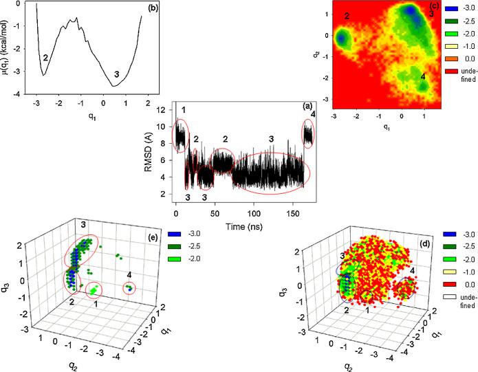
First we selected PCs, and found that the first four PCs belong to the multiply hierarchical category (not shown), and the percentage of the fluctuations captured by these PCs are ~14%, 12%, 7%, 6%, respectively. Figure 1 shows the RMSD as a function of time (a), and the FEL of the MD trajectory along the first (b), the first two (c) and the first three (d),(e) PCs, respectively. Panel (d) shows all points in the 3D FEL space with μ ≤ 0 kcal/mol, and the folding-unfolding pathways are not clearly illustrated in this plot because of strong overlapping of points corresponding to diverse energies. Therefore, we plotted the same 3D FEL with only the lowest free-energy points in panel (e). The numbers in each panel indicate the conformational states of the folding or unfolding trajectory. The one-dimensional FEL (b) possesses two pronounced minima (2 and 3), which represent non-native and native states, respectively. However, important information about the unfolded states at the beginning (1) and end (4) is missing because the first PC could not capture those parts of the MD trajectory. The unfolded state at the end of the MD trajectory (4) along with two other states (2, 3) are revealed in the 2D FEL (c); however, the 3D representation of the FEL (d),(e) is necessary to illustrate the complete “behavior” of the MD trajectory. Since the fourth PC also exhibits the multiply-hierarchical shape, the complete FEL must be four-dimensional. Since it is impossible to plot the 4D FEL, we made a table representation of multidimensional FELs up to five dimensions (Table I). Although the fourth PC is multiply hierarchical, we could not find any new major basins in the 4D FEL, which was hidden in the 3D FEL. The reason can be a slightly pronounced second minimum along the fourth PC. Since the fifth PC is singly hierarchical (not shown) [11], its pdf shape is Gaussian-like with a single peak and describes the fluctuations of the system within a specific conformational state; in the 5D FEL, only slight rearrangements of the coordinates of the minima of the non-native (2) and native (3) states are observed (Table I). Although, the FEL in a low-dimensional representation is not complete, the locations of the basins corresponding to the native/non-native states observed in 1D and 2D FELs are correct. Moreover, the activation barrier between non-native and native states in the multidimensional FELs (3D and higher) is ~2.2 times lower than in 1D and 2D FELs. This means that the folding pathway and kinetics can be incorrect in a low-dimensional representation. The diffusive behavior can also be misinterpreted. The diffusion of the protein in configurational space is anomalous [14] with two types: subdiffusion and super-diffusion. Since subdiffusion indicates that a system is trapped in local minima in conformational space, and superdiffusion emerges when the system makes long jumps in conformational space, the drastic change of the activation barrier height may cause the change of diffusion type.

FIG. 1.

(color online). (a) RMSD as a function of time, (b) 1D, (c) 2D, and (d), (e) 3D FELs (in kcal/mol) of 1BDD. The numbers in all panels correspond to the conformational states.

TABLE I.

Principal components of the minima of basins found in 1D, 2D, 3D, 4D, and 5D FELs. The numbers in the first column correspond to the conformational states in Fig. 1.

	1D	2D	3D	4D	5D
q1(3)	0.5	0.4	0.3	0.3	0.3
q1(2)	–2.7	–2.7	–2.7	–2.7	–2.7
q1(4)		0.9	0.9	0.9	0.9
q1(1)			0.1	0.1	0.1
q2(3)		1.2	1.3	1.3	1.3
q2(2)		–0.1	–0.1	–0.1	–0.3
q2(4)		–2.5	–2.5	–2.5	–2.5
q2(1)			–0.1	–0.1	–0.1
q3(3)			–0.3	–0.3	–0.5
q3(2)			–0.1	–0.1	0.1
q3(4)			–1.7	–1.7	–1.7
q3(1)			–1.9	–2.1	–2.1
q4(3)				0.3	0.3
q4(2)				–0.1	–0.1
q4(4)				1.3	1.3
q4(1)				–0.5	–0.5
q5(3)					0.5
q5(2)					–0.1
q5(4)					0.9
q5(1)					–1.7

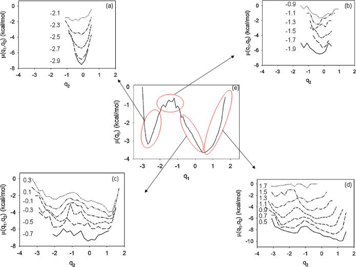
Another interesting finding of this study is related to “the similarities in the dynamics” of FELs along high- and low-indexed PCs. In other words, if we make slices along q₂ for each fixed q₁ of a 2D FEL [Fig. 1(c)], then the topography of these slices is similar to the topography of the 1D FEL along q₁ [Fig. 1(b)] at each state. For a clear illustration of these results, in Fig. 2 we clustered the slices of the FEL along q₂ for non-native (a), transition (b), and native (c),(d) states. The topography of the FEL slices along q₂ of the non-native (a) and transition (b) states is similar to the topography of the non-native and transition states of the FEL along q₁ (e), whereas most of the FEL slices along q₂ of the native state (c),(d) describe the shape of the entire FEL along q₁ (e). The reason for this difference is that the non-native and transition states are formed in the first part of the trajectory, i.e., before folding; consequently, the information about the native state is missing in the FEL of these parts. The native state is formed after folding and, consequently, contains information from the unfolded and transition parts. Therefore, the slices of the native state exhibit the complete shape of the FEL. This is the reason that this finding is called “the similarities in dynamics.”

FIG. 2.

(color online). 1D slices along q₂ [shifted from each other by 1 kcal/mol in μ(q₁, q₂) to avoid overlapping] for fixed q₁ of non-native (a), transition (b) and native (c,d) states, and 1D FEL along q₁ (e). The numbers in panels correspond to fixed q₁.

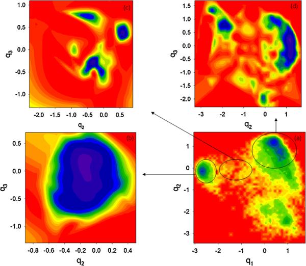
We extended our finding from 1D slices to 2D surfaces and plotted the surfaces in Fig. 3. We sliced the 3D FEL [Fig. 1(d)] in the 2D surfaces along q₂ and q₃ for fixed q₁. Comparing the 2D FEL along q₁ and q₂ (a) to FELs along q₂ and q₃ for non-native (b), transition (c) and native (d) states, we observe the same kinds of similarities as in Fig. 2. In other words, the topography of the 2D FEL slices along q₂ and q₃ of the non-native (b) and transition (c) states is similar to the topography of the non-native and transition states of the FEL along q₁ and q₂ (a), and the topography of the FEL slices along q₂ and q₃ of the native state (d) is similar to the topography of the entire FEL along q₁ and q₂ (a). We have done the same analysis for three other MD trajectories to make sure that the findings about similarities in dynamics are not accidental, and obtained the same kind of results. We think that these similarities can be caused by the correlations between the multiply hierarchical PCs [11], and the fractal nature of proteins [17–19]. The latter is a property common to all sufficiently large and anharmonic systems caused by the self-generated dynamical noise due to intermode coupling and equilibration promoted by anharmonic effects [17]. The inability to use a low-dimensional FEL is linked to coupling between hidden and representable dynamical processes that show up as fractal scales in the trajectories themselves.

FIG. 3.

(color online). 2D FEL (in kcal/mol) along q₁ and q₂ (a), and 2D FELs along q₂ and q₃ for fixed q₁ of non-native (b), transition (c), and native (d) states.

In our opinion, the problems addressed in this work are important for protein folding dynamics, especially for trajectories computed near the folding-transition temperature for which the system jumps between the folded, partially folded, and unfolded states. As was shown here, the FELs derived from such trajectories may be more complex than those derived from trajectories computed at lower temperatures at which the equilibrium population of the folded structure is almost 100% and for which the unfolded structures are virtually never visited after folding [14]. Therefore, it will be of interest to perform a similar analysis on other systems, and with other sets of order parameters to see whether our findings about the similarities of FELs along low- and high-indexed PCs are general features of proteins.

References

- 1.Frauenfelder H, Sligar SG, Wolynes PG. Science. 1991;254:1598. doi: 10.1126/science.1749933. [DOI] [PubMed] [Google Scholar]
- 2.Brooks CL, III, Onuchic JN, Wales DJ. Science. 2001;293:612. doi: 10.1126/science.1062559. [DOI] [PubMed] [Google Scholar]
- 3.Wales DJ. Energy Landscapes. Cambridge University Press; Cambridge, England: 2003. [Google Scholar]
- 4.Boczko EM, Brooks CL., III Science. 1995;269:393. doi: 10.1126/science.7618103. [DOI] [PubMed] [Google Scholar]
- 5.Liwo A, Khalili M, Scheraga HA. Proc. Natl. Acad. Sci. U.S.A. 2005;102:2362. doi: 10.1073/pnas.0408885102. [DOI] [PMC free article] [PubMed] [Google Scholar]
- 6.Jolliffe IT. Principal Component Analysis. Springer; New York: 2002. [Google Scholar]
- 7.Krivov SV, Karplus M. Proc. Natl. Acad. Sci. U.S.A. 2004;101:14766. doi: 10.1073/pnas.0406234101. [DOI] [PMC free article] [PubMed] [Google Scholar]
- 8.Altis A, et al. J. Chem. Phys. 2008;128:245102. doi: 10.1063/1.2945165. [DOI] [PubMed] [Google Scholar]
- 9.Hyeon C, Thirumalai D. J. Am. Chem. Soc. 2008;130:1538. doi: 10.1021/ja0771641. [DOI] [PubMed] [Google Scholar]
- 10.Mu Y, Nguyen PH, Stock G. Proteins: Struct. Funct. Genet. 2005;58:45. doi: 10.1002/prot.20310. [DOI] [PubMed] [Google Scholar]
- 11.Kitao A, Hayward S, Gō N. Proteins: Struct. Funct. Genet. 1998;33:496. doi: 10.1002/(sici)1097-0134(19981201)33:4<496::aid-prot4>3.0.co;2-1. [DOI] [PubMed] [Google Scholar]
- 12.Hegger R, Altis A, Nguyen PH, Stock G. Phys. Rev. Lett. 2007;98:028102. doi: 10.1103/PhysRevLett.98.028102. [DOI] [PubMed] [Google Scholar]
- 13.Macias MJ, Gervais V, Civera C, Oschkinat H. Nat. Struct. Biol. 2000;7:375. doi: 10.1038/75144. [DOI] [PubMed] [Google Scholar]
- 14.Maisuradze GG, Liwo A, Scheraga HA. J. Mol. Biol. 2009;385:312. doi: 10.1016/j.jmb.2008.10.018. [DOI] [PMC free article] [PubMed] [Google Scholar]
- 15.Gouda H, et al. Biochemistry. 1992;31:9665. doi: 10.1021/bi00155a020. [DOI] [PubMed] [Google Scholar]
- 16.Liwo A, et al. J. Phys. Chem. B. 2007;111:260. doi: 10.1021/jp065380a. [DOI] [PMC free article] [PubMed] [Google Scholar]
- 17.Lidar DA, Thirumalai D, Elber R, Gerber RB. Phys. Rev. E. 1999;59:2231. [Google Scholar]
- 18.Enright MB, Leitner DM. Phys. Rev. E. 2005;71:011912. doi: 10.1103/PhysRevE.71.011912. [DOI] [PubMed] [Google Scholar]
- 19.Reuveni S, Granek R, Klafter J. Phys. Rev. Lett. 2008;100:208101. doi: 10.1103/PhysRevLett.100.208101. [DOI] [PubMed] [Google Scholar]