How Direction of Illumination Affects Visually Perceived Surface Roughness

Abstract

We examined visual estimation of surface roughness using random computer-generated three-dimensional (3D) surfaces rendered under a mixture of diffuse lighting and a punctate source. The angle between the tangent to the plane containing the surface texture and the direction to the punctate source was varied from 50 to 70 degrees across lighting conditions. Observers were presented with pairs of surfaces under different lighting conditions and indicated which 3D surface appeared rougher. Surfaces were viewed either in isolation or in scenes with added objects whose shading, cast shadows and specular highlights provided information about the spatial distribution of illumination. All observers perceived surfaces to be markedly rougher with decreasing illuminant angle. Performance in scenes with added objects was no closer to constant than that in scenes without added objects. We identified four novel cues that are valid cues to roughness under any single lighting condition but that are not invariant under changes in lighting condition. We modeled observers’ deviations from roughness constancy as a weighted linear combination of these “pseudo-cues” and found that they account for a substantial amount of observers’ systematic deviations from roughness constancy with changes in lighting condition.

Roughness is a surface property that can be used to describe materials or to discriminate them, and it can be critical in the classification of materials. For example, Figure 1 shows sandpapers of different “grits”. One can readily discriminate the different grits both visually and haptically.

Figure 1. Surface roughness.

These are photographs of pieces of sandpaper of varying grit painted the same shade of gray. Illuminant direction is the same for all images. Notice that these sandpapers vary in perceived roughness.

For our purposes, roughness is an aggregate or statistical measure of the shape, size and distribution of elements on a surface. It may be classified haptically (Lederman & Klatzky, 2004) or visually (Rao & Lohse, 1993, 1996). Haptic psychophysical data indicate that perceived haptic roughness increases with an increase in the scale of surface elements. Parameters that affect haptic roughness include inter-element spacing and grating groove width (Klatzky & Lederman, 1999; Sathian, Goodwin, John, & Darian-Smith, 1989). Visually perceived roughness likely depends on the size and spacing of the many elements of which a textured surface (e.g., sandpaper) is composed. We are interested in the visual assessment of roughness in classes of surfaces similar to sandpaper or stucco. We refer to these surfaces as 3D textures.

Unlike 2D textures, the image of 3D textures changes with illumination and viewpoint conditions. Variations in the appearance of different samples of 3D texture can be captured by the Bidirectional Texture Function (BTF) of Dana, van Ginneken, Nayar, and Koenderink (1999), a function which summarizes the effects of changes in illumination and viewpoint conditions. Here we examine how visual estimates of roughness, a property inherent to 3D textures, depend on illumination.

Perception of Surface Roughness

Haptic perception of roughness in 3D textures is evidently unaffected by changes in illumination conditions and, if visual perception of the roughness of 3D textures were well-calibrated to haptic perception of the same textures, we might expect a high degree of roughness constancy across changes in lighting conditions. However, there are also good reasons to expect otherwise.

First, it is plausible that visual perception of 3D texture is closely related to shape perception, which is not invariant under changes in lighting conditions. There is evidence that the perception of surface relief (Belhumeur, Kriegman, & Yuille, 1999; Berbaum, Bever, & Chung, 1983; Oppel, 1856; Yonas, 1979) and shape estimated from shading (Koenderink, van Doorn, Christou, & Lappin, 1996a,b; Langer & Bülthoff, 2000) are far from invariant under changes in lighting conditions. Second, inspection of monocular images corresponding to a 3D texture suggests that perceived roughness varies markedly with lighting conditions. Figure 2 shows computer-rendered images of a monochrome matte surface viewed under two lighting conditions. On the left, the lighting is primarily diffuse; on the right, it is a mixture of diffuse and punctate illumination. Most observers would agree that the surface shown on the right appears rougher than the one on the left.

Figure 2. Rough surfaces.

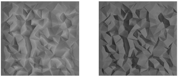
The same faceted surface is shown rendered under two different illuminants. One contains a primarily diffuse illuminant (left) and the other, a diffuse plus a punctate illuminant (right). Note that the images differ substantially; in particular, the right-hand surface appears somewhat rougher.

However, under binocular viewing conditions the viewer will have binocular disparity cues to roughness that are little affected by changes in lighting condition. It is plausible that observers would exhibit a higher degree of roughness constancy with binocular viewing.

Moreover, recent work examining surface color perception suggests that the constancy of judgments of surface color and lightness perception increases when the scene contains cues such as shadows and specular highlights that signal the spatial and spectral distribution of the illumination (Boyaci, Doerschner, & Maloney, 2004; Boyaci, Maloney, & Hersh, 2003; Doerschner, Boyaci, & Maloney, 2004; Ripamonti et al., 2004; Yang & Maloney, 2001). Such judgments improve as more cues to the illumination conditions are provided (Boyaci, Doerschner, & Maloney, 2006; Kraft, Maloney, & Brainard, 2002; Yang & Maloney, 2001).

We conjecture that failures of roughness constancy observed when a surface is judged in isolation may be due to lack of information about illumination geometry. Koenderink and colleagues (2003) suggest that cues available in images of surfaces are not sufficient to accurately estimate the azimuth and elevation of a collimated light source. In particular, they found that, for obliquely illuminated textured surfaces, observers could estimate the azimuth of the source to within about 15° (if we ignore frequent 180° confusions) while estimates of elevation were barely better than chance. We know that these ambiguities are almost completely resolved in real scenes containing other objects and landmarks. By adding context to the scene we could thereby provide more cues—such as shadows and specular highlights—to illumination conditions. This could lead to a greater degree of roughness constancy.

Preview

In the present study, we examine perception of the roughness of 3D textures, binocularly-viewed, under changes in the direction of a punctate illuminant. Our goal is to investigate what factors in the scene determine failures in roughness constancy with changes in lighting conditions. We compare conditions where only the 3D texture is available to conditions where we have additional illuminant cues.

Methods

Stimuli

Coordinate systems

The stimuli were defined using a Cartesian coordinate system (x,y,z) (Figure 3). The origin (0,0,0) is in the fronto-parallel plane on which we present stimuli (the stimulus plane). The z-axis lies along the observer’s line of sight. The x-axis is horizontal and the y-axis is vertical. The punctate illuminant direction is represented as a vector P using spherical coordinates (ψ,ϕ,d). We define elevation ϕ as the angle between P and the projection of P on the xy-plane; it ranges from 0 to 90°. The azimuth ψ is the angle between the projection of P onto the xy-plane and the x-axis.

Figure 3. Coordinate systems.

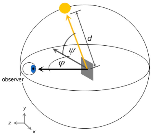
Cartesian coordinate system was used in defining surface patches. The z-axis lies along the line of sight from the observer to the origin such that the observer’s gaze is in the -z direction. The x-axis lies along the horizontal line tangential to the surface and the y-axis lies along the vertical line tangential to the surface. For the punctate illuminant positions, spherical coordinates were used. The illuminant had an elevation ϕ (relative to the surface) and azimuth ψ, and was located at a distance d from the surface patch. In this study, ϕ was varied while ψ and d were fixed at 180° and 80 cm, respectively. The origin of the coordinate system was the center of the surface patch. The observer was always at (x,y,z) = (0,0,70 cm) or, in spherical coordinates, (ψ ϕr)= (90°,−,70 cm).

Surface patch

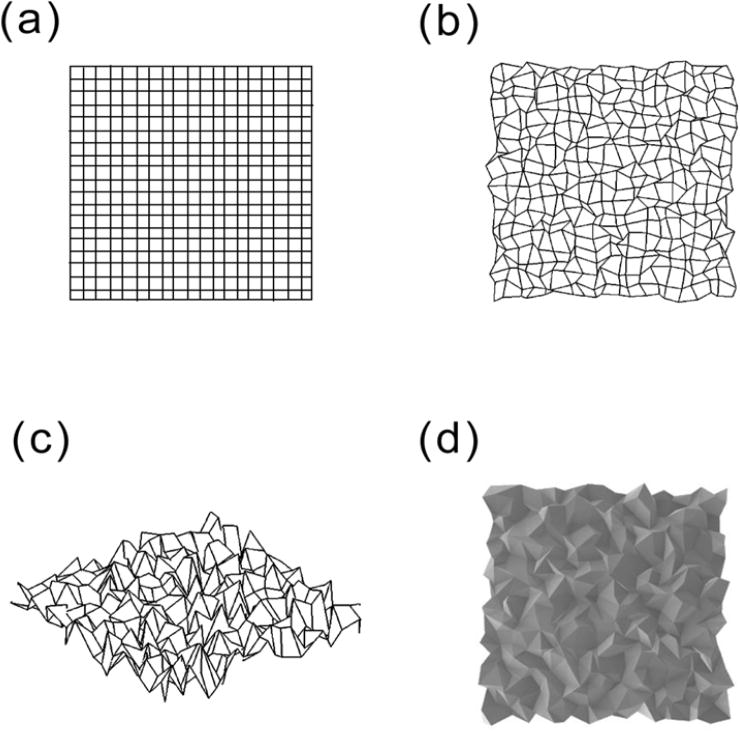
Our 3D textured surfaces were composed of randomly-oriented Lambertian facets. Figure 4 illustrates how surface patches were constructed. First, an N×N grid of base points was generated in the stimulus plane with width w. The base point coordinates are denoted (X_ij,Y_ij,Z_ij), 0 ≤ i, j ≤ N − 1. Let $U_{ij}^x,U_{ij}^y,U_{ij}^z$ be independent, uniformly distributed random variables on the interval [−1,1]. The base point coordinates were defined as

Figure 4. Rough surface model.

(a) A 19×19 cm regular grid of 20×20 base points was constructed. (b) The base points of the grid were jittered randomly in the x-y plane. (c) Uniform random deviations were added to the base points in the z direction. (d) The surface comprised of 3D jittered base points was then divided into triangular facets by randomly splitting each 2×2 set of base points along a diagonal.

$$\begin{array}{l}{X}_{ij}=-\frac{w}{2}+\left(j+n_{xy}{U}_{ij}^x\right)\delta \\ Y_{ij}=-\frac{w}{2}+\left(i+n_{xy}{U}_{ij}^y\right)\delta \\ Z_{ij}={rU}_{ij}^z,\end{array}$$ (1)

where w=19 cm, $\delta =\frac{w}{N-1}$, and the grid has N=20 points on a side. Setting n_xy = 0.49 ensured that no facets would overlap or intersect one another in the jittered base grid. The amount of jitter in depth could take on any of eight distinct values r = k²/16 cm depending on the roughness level k = {1,2,···,8}. The standard deviation of the Z_ij coordinates in a surface with roughness level r was $\sqrt{3}{k}^2/12\text{cm}$. A flat surface, r = 0, would thus mean all Z_ij = 0. The Z_ij coordinates were always 4 cm or less in absolute value. Note that the spacing of the standard deviation of successive roughness levels is quadratic in r. In initial testing we found that linear spacing led to stimuli that were difficult to discriminate at high roughness levels and we consequently adopted quadratic spacing. The 3D surface was constructed from triangular facets. Each set of four neighboring grid points (i, j), (i +1, j), (i, j +1), and (i +1, j +1) was split into two triangular facets by randomly selecting one of the two diagonals to be connected by an edge. For each value of roughness, illuminant elevation and context condition (see Illuminant cues), four random surfaces were generated to minimize the possibility of observers using patterns in the distribution of facets as cues to roughness.

Light sources

Each surface patch was rendered under a diffuse plus punctate illuminant using the RADIANCE rendering software package (Larson & Shakespeare, 1996; Ward, 1994; http://radsite.lbl.gov/radiance/HOME.html). The surface facets were Lambertian with albedo 0.5. They were rendered with interreflections (one ambient bounce) as well as occlusions and vignetting. All surfaces were oriented frontoparallel to the observer. The punctate illuminant had azimuth ψ =180° (light came from the left) and elevation ϕ=50, 60 or 70° (Figure 5). It was located 80 cm away from the surface and the punctate-total ratio was 0.62.¹

Figure 5. Punctate illuminant directions.

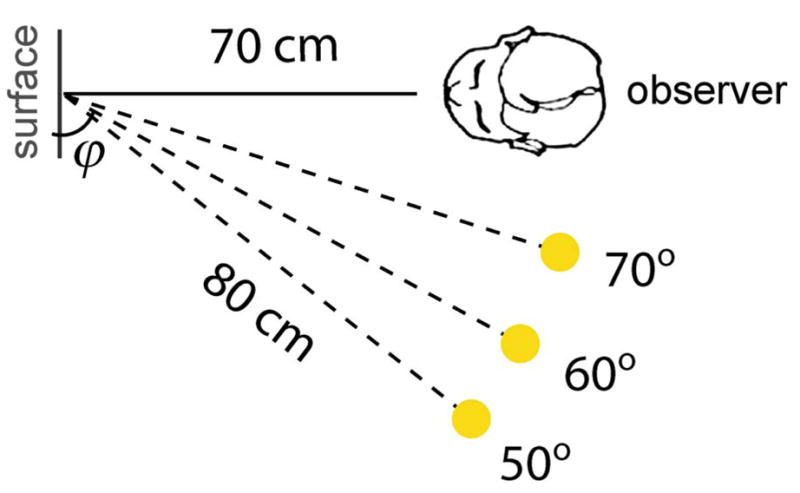
Three illuminant elevations (ϕ =50°, 60°, 70°) were used in this study.

To prevent cues that may result from an abrupt change in depths of the edges of the surface patch and the wall, a 3.6 cm border around the surface patch was multiplied by a raised cosine function to smooth the edges of the surface in depth. A “woodgrain” patterned floor was present in both the control and experimental conditions to provide more cues to depth.

Illuminant cues

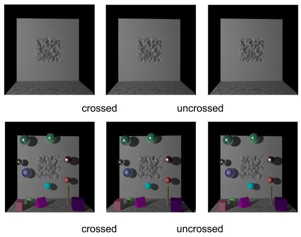
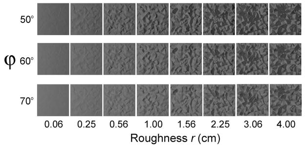
There were two context conditions. In Condition I (Figure 6, top panel), the rough surface patch was embedded in a flat wall and the only other visible surface was a textured floor. In Condition II (Figure 6, bottom panel), additional objects were added to the scene including cubes, prisms, and cylinders resting on the floor, and floating spheres. These objects had varying colors, degrees of specularity, and positions in the scene. Each scene was then rendered from two different viewpoints (±3 cm) and viewed binocularly. A representative set of surface patches with varying roughness and illuminant elevation is shown in Figure 7.

Figure 6. Stereo pair of stimuli.

Two example stimuli of roughness level r = 2.25 are shown corresponding to Condition I (top row) and Condition II (bottom row). The two images on the left can be used for crossed fusion and two images on the right can be used for uncrossed fusion.

Figure 7. Examples of Stimuli.

For each roughness level, four surfaces were generated. Here, one of the four is shown for each roughness level r rendered under each of the three punctate illuminant directions.

Apparatus

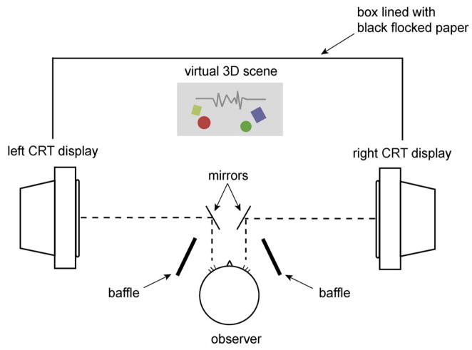
The left and right images were presented to the corresponding eye of the observer using two 21” Sony Trinitron Multiscan GDM-F500 monitors in a mirror stereoscope (Figure 8). The screens on these monitors are close to physically flat, with less than 1 mm of deviation across the surface of each monitor. Look-up tables were used to correct display nonlinearities and to equate the luminance on the two displays based on measurements of the luminance values on each monitor made with a Photo Research PR-650 spectrometer. The maximum luminance achievable on either screen was 114 cd/m². The stereoscope was contained in a box 124 cm on a side. The front face of the box was missing and that is where the observer sat in a chin/head rest. The interior of the box was coated with black flocked paper (Edmund Scientific, Tonawanda, NY) to absorb stray light. Only the stimuli on the screens of the monitors were visible to the observer. The casings of the monitors and any other features of the room were hidden behind the non-reflective walls of the enclosing box.

Figure 8. The experimental apparatus.

Stimuli were displayed using a Wheatstone stereoscope. The left and right images of a stereo pair were displayed on the left and right monitors. The observer viewed them via small mirrors placed in front of his or her eyes. In the fused image, the surface patch appeared approximately 70 cm in front of the observer. The distance was also the optical distance to the screens of the two computer monitors, minimizing any mismatch between accommodation and other distance cues.

Additional light baffles were placed near the observer’s face to prevent light from the screens reaching the observer’s eyes directly. The optical distance from each of the observer’s eyes to the corresponding computer screen was 70 cm. To minimize any conflict between binocular disparity and accommodation, the stimuli were rendered to be 70 cm in front of the observer. The monocular fields of view were 55×55°. The observer’s eyes were approximately in line with the center of the scene being viewed.

The experimental software was written in the C programming language using the X Window System, Version 11R6 (Scheifler & Gettys, 1996) running under Red Hat Linux 6.1 for graphical display. The computer was a Dell 410 Workstation with a Matrox G450 dual head graphics card and a special purpose graphics driver from Xi Graphics that permitted a single computer to control both monitors. The monitors were synchronized by a common signal from the Matrox board. The rendered stereo image pair was represented by floating point RGB triplets for each pixel of the image. These triplets were the relative luminance values of each pixel. We translated these values to 24-bit graphics codes, correcting for nonlinearities in the monitors’ responses by means of look-up tables.

Procedure

We used a two-interval forced-choice discrimination paradigm in which a test surface patch and a match surface patch were presented and the observer’s task was to indicate which patch appeared to be rougher. The test, under one illuminant, was chosen from the intermediate range of roughness levels (0.25 ≤ r ≤ 3.06 cm, see Figure 7), whereas the match was under a different illuminant and could have any of the 8 roughness levels.

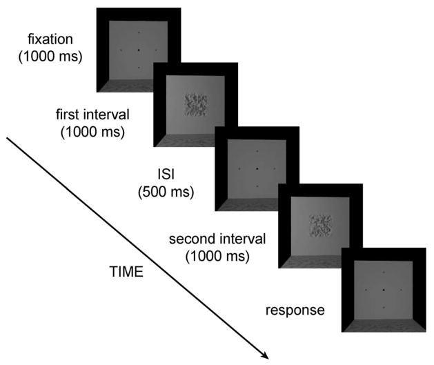
Figure 9 illustrates the sequence of events in a trial. The observer first saw a gray surface containing a central fixation point and four flanking black dots for 500 ms at the same depth at which the patch would appear. The flanking dots were included to help observers maintain fusion. Then a test or match stimulus appeared for 1000 ms in the first interval of each trial. The fixation stimulus reappeared during the 500 ms interstimulus interval, and then a second test or match stimulus was presented for 1000 ms in the second interval. The observer responded by pressing either the right or left mouse button for the corresponding interval that s/he believed to contain the rougher patch. The next trial was presented immediately after a response was made. The test stimulus was randomly displayed in the first or second interval and the match was displayed in the other. For each type of comparison (test patch roughness level, test and match illumination conditions), two types of staircases were used (“2-up, 1-down” and “1-up, 2-down”) to determine the roughness level of the match surface. Points of subjective equality (PSEs; i.e., points at which the match was perceived rougher than the test 50% of the time) were estimated by combining the data from the two types of adaptive staircases. This resulted in a total of 72 interleaved staircases (6 test roughness levels 3 illuminant comparisons × 2 staircase types × 2 context conditions). Each observer completed 20 trials per staircase. These trials were split into two sessions; the staircases were continued across sessions.

Figure 9. Trial sequence.

The observer performed a two-interval forced-choice task in which a test surface appeared in one interval and a match surface appeared in the other interval. When no stimulus was displayed, observers viewed a central fixation point flanked by four dots positioned on a surface that appeared with the same disparity as the stimulus surface so that observers could maintain vergence at the appropriate distance. Observers indicated which patch appeared rougher. The next trial was presented after a response was made. Observers were permitted as much time as necessary to make a response.

Observers

Seven observers participated. Three observers were naïve; four (YXH, MSL, CP, and JF) were aware of the purpose of the experiment. All observers had normal or corrected-to-normal vision.

Results

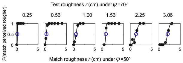
A representative set of psychometric functions collected for one observer are shown in Figure 10. PSEs were obtained by fitting the data with a Weibull distribution and estimating the point at which there was a 50% probability of choosing the match surface as rougher.

Figure 10. Psychometric functions.

A representative set of psychometric functions obtained for one observer for the comparison of a test surface patch under illuminant elevation ϕ= 70 compared to a match surface patch under ϕ = 50. The data were fit with a Weibull distribution (black line) and the point at which the match surface appeared rougher than the test surface 50% of the time (the point of subjective equality or PSE) was estimated from a total of 40 trials per psychometric function (blue circles).

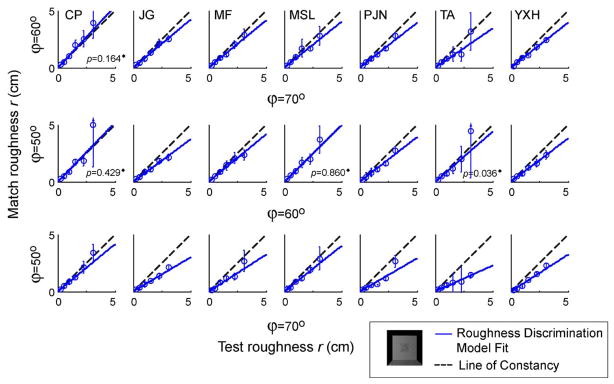
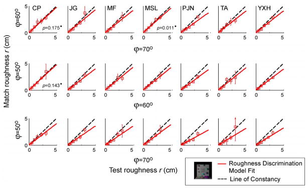
Results for all observers are shown in Figures 11 and 12. The 95% confidence intervals for each PSE were obtained by a bootstrap method (Efron & Tibshirani, 1993) whereby each human observer’s performance in the corresponding condition was simulated 1000 times and the 5^th and 95^th percentiles were calculated.

Figure 11. Results for Condition I.

PSEs are plotted for each pair of illuminant conditions for seven observers. The dashed line represents the results expected of a roughness-constant observer. The solid lines are linear fits to the data predicted by the roughness discrimination model. 17 out of 21 slopes predicted by the linear model were significantly different from 1 (at the Bonferroni-corrected α level of 0.007 per test). Error bars represent bootstrapped 95% confidence intervals. (◆ indicates a fit that is not significantly different from the line of constancy.)

Figure 12. Results for Condition II.

Details as in Figure 11. 18 out of 21 of the slopes predicted by linear model were significantly different from 1 (at the Bonferroni-corrected α level of 0.007 per test). (◆ indicates a fit that is not significantly different from the line of constancy.)

If observers were roughness constant across changes in illumination, then their true PSEs should lie along the line of roughness constancy (i.e., the identity line) and the measured PSEs should show no patterned deviation from the line. Almost all PSEs fell below the line of roughness constancy. This trend strongly suggests that a surface appears rougher when illuminated from a more grazing angle.

Additional contextual cues do not improve roughness constancy

Surprisingly, we did not find any significant difference between Conditions I and II (Bonferroni-corrected α level for seven tests (α ≅ .007) for a z test of difference of slopes for the three illuminant comprisons). Thus, the additional cues to the illuminant direction provided in Condition II did not improve observers’ judgments of roughness across varying illumination conditions (Figure 13).

Figure 13. Results for Condition I compared to Condition II.

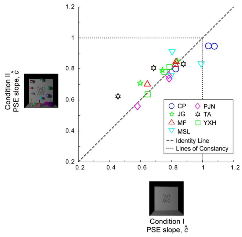
Estimates of the PSE slopes from Condition I are plotted versus those from Condition II for each observer. Each data point represents a comparison of all surfaces with varying roughness under two different illuminant conditions (e.g., ϕ = 70 vs. 50°) for a given observer. The dotted line represents the lines of roughness constancy along which points representing slope values of 1 would lie. The dashed line represents the identity line along which slope values for Conditions I and II would be equal to one another. Notice that almost all points lie inside the area inscribed by the lines of roughness constancy, indicating that almost all PSE slopes were less than one. Furthermore, all points lie roughly along the identity line.

Given this unexpected outcome, we sought to verify that the illuminant directions that we used were discriminable. In an experiment using identical methodology and only Condition II stimuli, one subject (YXH) readily identified the larger illuminant elevation, for a 10° difference between illuminant elevation angles, 93% of the time. We cannot explain the lack of effect of the additional cues to illuminant direction provided in Condition II as simply a failure of discrimination.

A model of roughness discrimination

Most PSEs fell below the line of roughness constancy. Thus, it seems that observers failed to display roughness constancy across varying illuminant directions. We modeled observers’ choice data to determine how much observers’ estimates were altered by the change of illuminant elevation. We assumed that an observer’s roughness discriminations were a function of (1) a roughness transfer parameter c (i.e., the slope of a linear fit to the data in Figures 11 and 12), (2) the standard deviation of normally-distributed noise that causes the variability in observers’ judgments, and (3) a noise scaling parameter γ. We assume that the noise is scaled by r^γ, thus if γ = 0, this corresponds to stimulus-independent noise. If γ = 1, this corresponds to Weber’s law for our roughness scale r (see Appendix for details). We denote the three illuminant conditions by A, B, and C (corresponding to illuminant elevations ϕ =70, 60, and 50°, respectively), resulting in three roughness transfer parameters c_AB, c_BC and c_AC, plus σ and γ, for a total of five model parameters. We estimated these parameters by maximum likelihood.

We first tested the hypothesis that the transfer parameters were all equal to 1 for each observer (i.e., roughness constancy). We rejected this hypothesis for 35 of the 42 transfer parameters for all seven observers (slope estimates ĉ were significantly less than 1 at the Bonferroni-corrected α level for seven tests, α ≈ .007). This outcome is not particularly surprising since we have little reason to expect perfect roughness constancy; however, what is of interest is the magnitude of the failure of roughness constancy across observers. The estimates of the roughness transfer parameter c were 0.78 on average, markedly less than 1. Additionally, most values of γ fell very close to 1 for all observers suggesting that noise increases in a manner that follows Weber’s Law with increasing levels of roughness (Table 1).

Table 1. Estimated roughness discrimination model parameter values for each observer for each condition.

Notice that almost all estimated PSE slope values (ĉ) are under 1 and most values of γ̂ are close to 1. Bold indicates a fit that is significantly different from the line of constancy at the Bonferroni-corrected α level of 0.007.

Context Condition	Model Parameter	Observer
		CP	JG	MF	MSL	PJN	TA	YXH
I	ĉ70°60°	1.074	0.840	0.826	0.802	0.783	0.688	0.787
	ĉ60°50°	1.037	0.743	0.828	0.991	0.779	0.872	0.757
	ĉ70°50°	0.826	0.599	0.646	0.797	0.582	0.453	0.648
	σ̂	0.462	0.354	0.398	0.479	0.392	0.795	0.269
	γ̂	0.976	0.967	0.944	0.980	0.990	0.979	0.972
II	ĉ70°60°	0.944	0.848	0.825	0.912	0.737	0.808	0.813
	ĉ60°50°	0.947	0.792	0.846	0.834	0.759	0.831	0.780
	ĉ70°50°	0.800	0.708	0.700	0.757	0.559	0.620	0.635
	σ̂	0.397	0.438	0.481	0.365	0.404	0.698	0.299
	γ̂	0.980	0.980	0.960	0.981	0.996	0.984	0.974

Testing transitivity

We tested whether the data display transitivity. That is, if one surface under illuminant A was perceived equal in roughness to another surface under illuminant B and that second surface was perceived equal in roughness to yet a third surface under illuminant C, then the transitivity prediction is that the first surface (under illuminant A) should match the third surface (under illuminant C). More specifically, if r_A is the roughness of any surface under illuminant A, and it matches a surface with roughness r_B under illuminant B, then

$$r_B=c_{AB}{r}_A.$$ (2)

If we now find the surface roughness under illuminant C that matches this second surface under illuminant B, we have,

$$r_C=c_{BC}{r}_B$$ (3)

and, combining Equations 2 and 3, we have the prediction,

$$r_C=c_{BC}{c}_{AB}{r}_A.$$ (4)

However, we also have the prediction, based on the model developed above, that

$$r_C=c_{AC}{r}_A.$$ (5)

Comparing Equations 4 and 5, we have the transitivity prediction,

$$c_{AC}=c_{BC}{c}_{AB}.$$ (6)

Since we have independent estimates of each of the transfer parameters, we can test whether Equation 6 is valid for our data.

Figure 14 shows the estimated values of slope ĉ_70°60° plotted against the corresponding slope predictions ĉ_60°50° ĉ_70°60° based on transitivity. Most of the data fall along the identity line. We estimated 95% confidence intervals for both prediction and estimate by a bootstrap method (Efron & Tibshirani, 1993).

Figure 14. Results.

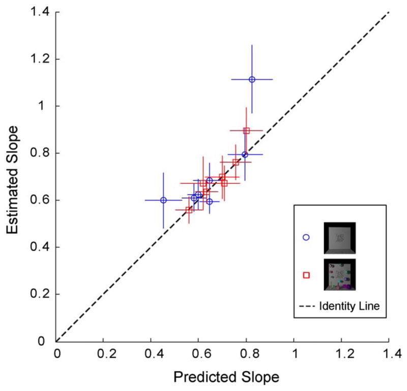
Estimated slopes, ĉ_70°50°, compared to slopes predicted by the transitivity rule, ĉ_60°50° ĉ_70°60°, for all observers in Conditions I (blue) and II (red). Standard errors represent 95% confidence intervals for each bootstrapped slope. For almost all points, the slopes match the predictions (dashed line).

The estimated and predicted values, their respective percentage error of prediction $\left(\epsilon =\frac{{\widehat{c}}_{60°50°}{\widehat{c}}_{70°60°}-{\widehat{c}}_{70°50°}}{{\widehat{c}}_{60°50°}{\widehat{c}}_{70°60°}}\times 100\%\right)$, and p-values are listed in Table 2. We performed a z test to determine whether the measured and predicted slopes were significantly different from each other for each possible comparison. There was no significant difference between slopes for both conditions (I and II) at the Bonferroni-corrected α level for seven tests (α ≈ .007) for 6 of the 7 observers, consistent with the claim that observers’ judgments are transitive.

Table 2.

Estimated values of slope ĉ_70°50° for each observer and predicted slope ĉ_60°50° ĉ_70°60° based on the transitivity rule (Equation 6). The error of prediction ε (see Testing transitivity for details) represents how much the estimated value of the slope departed from the value predicted by transitivity. Bold indicates a significant difference between slope values for a z test at the Bonferroni-corrected α level 0.007 per test.

Context Condition	Transitivity Predictions	Observer
		CP	JG	MF	MSL	PJN	TA	YXH
I	ĉ70°50°	0.826	0.599	0.646	0.797	0.582	0.453	0.648
	ĉ60°50° ĉ70°60°	1.113	0.624	0.684	0.794	0.610	0.600	0.596
	%ε	25.770	3.980	5.630	−0.300	4.640	24.560	−8.750
	p	0.001	0.540	0.453	0.972	0.480	0.041	0.126
II	ĉ70°50°	0.800	0.708	0.700	0.757	0.559	0.620	0.635
	ĉ60°50°ĉ70°50°	0.894	0.672	0.698	0.761	0.559	0.671	0.635
	%ε	10.480	−5.380	−0.370	0.490	0.010	7.610	−0.002
	p	0.131	0.473	0.966	0.941	0.999	0.497	~1

Discussion

In this study, we found that observers deviated substantially from the predictions of roughness constancy. Figure 15 shows two rendered surfaces that a typical observer perceived to be equal in roughness. This deviation from roughness constancy held even after additional cues to illuminant direction were provided in the scene.

Figure 15. Two surfaces perceived by one observer (PJN) in this study to be equal in roughness.

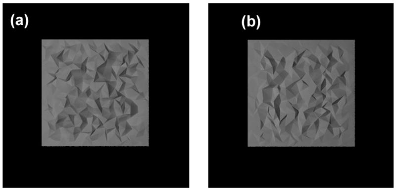
A fronto-parallel view of (a) a test surface with roughness r=1.56 cm under one illuminant (ϕ = 70°) and (b) a match surface with roughness r = 0.61 cm under another illuminant (ϕ = 50°), that was perceived to be equal in roughness to the surface in (a).

One explanation for the continued bias in responses with additional illuminant cues may be that observers did not have sufficient time to scrutinize the scene. It is possible that observers may have needed more than the one-second presentation time to process all the information in the relatively complex scene. We tested this possibility: One observer (YXH) repeated the experiment with each scene presented for two seconds instead of one. The bias remained: the estimated slopes (ĉ values) for Conditions I and II were nonzero and less than 1 (z tests, p < 0.001).

Rather, we suggest that the additional cues in the scene do not improve roughness constancy because observers are instead relying on cues contained in the texture itself (as suggested by Koenderink et al., 2003). That is, observers may use the pattern of shading and cast shadows to estimate surface roughness. These cues vary with roughness, but also vary with changes in the pattern of illumination, leading to failures of roughness constancy.

A cue combination model

In an image of a 3D surface, there exist a number of visual cues that are affected by changes in surface roughness. Some of these are invariant under changes in illumination conditions and others are not. An example of the former would be a measure of the depth variance of the surface patch based on disparity estimates. So long as the visual system can accurately estimate disparity values, this information should not be affected by changes in lighting. Let R_d denote the estimate of roughness based on illumination-invariant cues. Note that R_d may be the result of combining multiple illumination-invariant cues. For our purposes, it suffices to lump all such cues together.

We assume that the expected value of R_d is the true roughness of the surface: E(R_d) = r. That is, R_d is an unbiased cue. If a visual system used only R_d as its roughness estimate, then it would display roughness constancy. However, if the variance of R_d is large, then the observer’s estimates would be highly variable from trial to trial. Consequently, the observer might seek to reduce the variance by combining R_d with other roughness cues. These additional cues are necessarily affected by change in illumination, given how we have defined R_d.

Inspection of the rendered images suggests four physical measures of the scene that would be affected by changes in roughness r: (1) r_p: the proportion of the image that is not directly lit by the punctate source (the proportion of the image in shadow) (2) r_s: the standard deviation in luminance of non-shadowed pixels in the image due to differential illumination by the punctate source, (3) r_m: the mean luminance of non-shadowed pixels, and (4) r_c: texture contrast² as defined by Pont & Koenderink (2005). Texture contrast is intended to be a robust statistic for characterizing materials across lighting conditions. It is less sensitive to lighting changes than the other three measures. Each measure is a function of the true roughness of the surface r and the lighting condition L and can be written r_s(r, L), r_m(r, L), r_p(r, L), and r_c(r, L) to emphasize this dependence.

Each of these measures is highly correlated with roughness r when only roughness is varied while the lighting condition L is held constant. Increasing roughness, for example, increases the proportion of the scene r_p(r, L) consisting of cast and attached shadows. Correspondingly, the mean image intensity decreases and the variation of facet illumination increases. We have verified that this is the case in our stimuli for all four of these measures. However, when surface roughness remains constant and lighting conditions change the values of these measures also change. Consequently, the values of these measures confound roughness and lighting condition.

We assume that the visual system has available four “pseudo-cues” to roughness, R_s, R_m, R_p, and R_c corresponding to the four physical measures just defined. We assume that each is an unbiased estimate of the corresponding physical measure, i.e., E[R_p]= r_p(r, L) and similarly for the other three measures.

We consider the possibility that the visual system errs in using these pseudo-cues across changes in lighting condition. We assume that cues and pseudo-cues are scaled and combined by a weighted average (Landy, Maloney, Johnston, & Young, 1995). In viewing a surface of roughness r in lighting condition L, the observer forms the roughness estimate

$$R=w_d{R}_d+w_s{R}_s+w_m{R}_m+w_p{R}_p+w_c{R}_c,$$ (7)

where the values w_i combine the scale factors and weights, and thus need not sum to one as weights do.

In this experiment, observers compare this roughness estimate to the roughness estimate for a second surface patch with roughness r′ viewed under a different lighting condition L′,

$$R^{\prime }=w_d{R}_d^{\prime }+w_s{R}_s^{\prime }+w_m{R}_m^{\prime }+w_p{R}_p^{\prime }+w_c{R}_c^{\prime },$$ (8)

to decide which surface was rougher. Consider the situation in which two surfaces are perceived as equally rough, i.e., R = R′. Subtracting Equations 7 and 8 yields

$$0=w_d\mathrm{\Delta }{R}_d+w_s\mathrm{\Delta }{R}_s+w_m\mathrm{\Delta }{R}_m+w_p\mathrm{\Delta }{R}_p+w_c\mathrm{\Delta }{R}_c,$$ (9)

where $\mathrm{\Delta }{R}_i=R_i^{\prime }-R_i$. We assume that w_d is non-zero (the observer is making some use of illuminant-invariant cues) and rearrange as

$$\mathrm{\Delta }{R}_d=a_s\mathrm{\Delta }{R}_s+a_m\mathrm{\Delta }{R}_m+a_p\mathrm{\Delta }{R}_p+a_c\mathrm{\Delta }{R}_c,$$ (10)

where a_s = −w_s/w_d, etc. If R_s, R_m, R_p and R_c were unbiased cues to roughness then the expected values of ΔR_s, ΔR_m, ΔR_p, and ΔR_c would all be 0 and, as a consequence, E[ΔR_d] = r − r′ = 0. We would expect the observer to be roughness constant on average, but that is not what we found experimentally. Observers systematically matched surfaces with very different roughness r ≠ r′ across lighting conditions.

The expected value of the difference between the pseudo-cue R_p and $R_p^{\prime }$ is the difference between the actual proportion of the image not directly lit by the punctate illuminants in the two scenes. If we denote this difference by Δr_p = r_p(r′,L′) − r_p(r, L), then we have E[ΔR_p] = Δr_p. Similarly, E[ΔR_m] = Δr_m, E[ΔR_s] = Δr_s, and E[ΔR_c]= Δr_c.

We computed the expected values of each of the terms Δr_s, Δr_m, Δr_p, and Δr_c for each value of roughness and lighting condition by first computing r_s(r, L), r_m(r, L), r_p(r, L), and r_c(r, L) for each possible roughness r and lighting condition L and then taking differences. These were computed using the four stimulus images for each condition.

To compute r_p, r_m, and r_s we must determine which pixels in each image are not directly illuminated by the punctate source. To do this, we re-rendered our scenes with the diffuse lighting term set to 0 and surface albedo set to 1 and no interreflections among facets. We refer to these re-rendered images as punctate-only images.

Pixels with a value of 0 in a punctate-only image correspond to surfaces that are not directly illuminated by the punctate source (i.e., in shadow). The proportion of shadowed pixels (r_p) and the other terms based on non-shadowed pixels (r_m and r_s) are easily computed once we know which pixels in the image are not directly illuminated by the punctate source. We determined the set of shadowed pixels using the left-eye images only.

Equation 10 posits that the difference in roughness at the PSE is a linear combination of the difference in each of the cues we have identified, each perturbed by error. To test this model, we collapsed Conditions I and II and regressed 36 PSE differences (2 context conditions × 3 illuminant comparisons × 6 test roughness levels) against the differences in the illuminant-variant cues. The resulting regression equation expresses the observers’ failures of constancy in terms of the hypothetical light-variant cues,

$$\mathrm{\Delta }{R}_d=a_s\mathrm{\Delta }{r}_s+a_m\mathrm{\Delta }{r}_m+a_p\mathrm{\Delta }{r}_p+a_c\mathrm{\Delta }{r}_c+a_0+\epsilon ,$$ (11)

where the error term combines all of the errors given by all terms in the model. The results of the regression fit are shown in Table 3. Note that we include a constant term a₀ in the regression. We will return to this term in the discussion below.

Table 3. Percentage of variance (R²) accounted for by combinations of predictors regressed to deviations in roughness.

(ΔR_d). For each row, we tested the null hypothesis that R² = 0 for each entry in the table, with a Bonferroni correction for multiple tests. Bold indicates that R² was significantly different from 0. The overall α of the test was 0.05. The Bonferroni-corrected level for each was 0.007 = 0.05/7. We did not apply Bonferroni correction for all 49 tests as the results in each column are not independent.

VAF	Observer
	CP	JG	MF	MSL	PJN	TA	YXH
$R_c^2$	35	57	45	40	34	25	70
$R_s^2$	63	41	32	42	19	30	45
$R_m^2$	2	17	19	16	15	8	18
$R_p^2$	12	15	24	14	29	2	57
$R_{s,c}^2$	71	58	47	43	41	30	80
$R_{m,c}^2$	44	58	45	40	34	26	70
$R_{m,s}^2$	72	41	33	42	22	30	46
$R_{p,c}^2$	73	57	45	43	40	32	78
$R_{p,s}^2$	73	48	37	42	37	30	72
$R_{p,m}^2$	19	29	37	24	43	10	71
$R_{m,s,c}^2$	74	59	47	44	41	30	81
$R_{p,s,c}^2$	73	61	51	43	42	32	81
$R_{p,m,c}^2$	81	58	45	47	44	32	78
$R_{p,m,s}^2$	77	49	40	43	44	30	76
$R_{p,m,s,c}^2$	82	66	53	48	44	33	81

In using the variation in the cues from trial to trial to estimate the weight assigned to each cue we are, in effect, applying the technique used by Ahumada and Lovell (1971) that is the basis of image classification methods. Note that these coefficients do not provide us directly with an estimate of how much weight the observers give each cue. However, we can determine how much each cue or combination of cues contributes to the observer’s judgments by comparing the proportion of variance accounted for by each of the 15 possible combinations of predictors (Table 3). The combination of the four predictors of roughness judgments explains 58% of the variance in the data on average over the seven observers (values for individual observers ranged from 33 to 82%). Figure 16 shows ΔR_d (the observer’s failure of roughness constancy) plotted against the predicted values ΔR̂_d= â_sΔr_s + â_mΔr_m + â_pΔr_p + â_cΔr_c using regression estimates of the coefficients for the four pseudo-cues but without the constant term â₀. Most values fall close to the identity line. Although the values of â₀ were significantly different from 0 for some observers, the values of â₀ were relatively small and not patterned across observers. Hence we recomputed the regression, forcing â₀ to be 0.

Figure 16. Results.

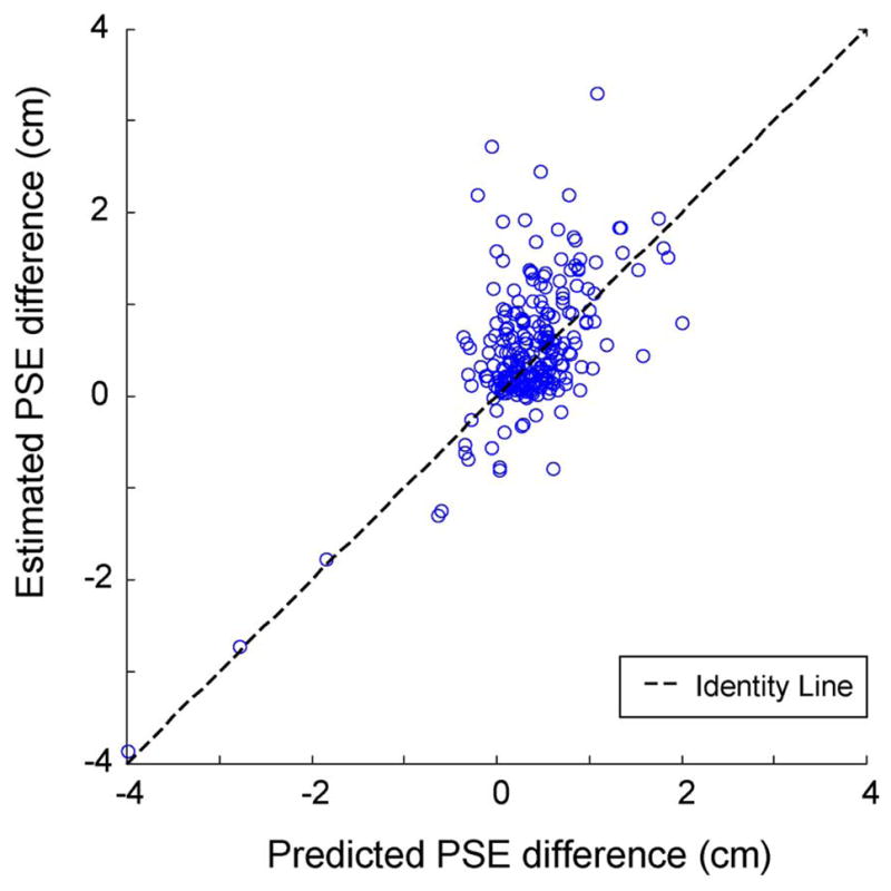
Estimated PSE difference as a function of PSE difference predicted by the linear cue combination model. Notice that most points fall roughly along the identity line. Positive values indicate PSEs falling below the line of roughness constancy. Data from Conditions I and II were collapsed and fitted together.

To summarize, if observers relied solely on illuminant-invariant cues, such as binocular disparity, to make roughness estimates, they would have exhibited no patterned deviations from roughness constancy. Instead, it seems that observers relied on other measures in the scene such as the four pseudo-cues we considered. These pseudo-cues do not provide accurate information about roughness across lighting conditions. The visual system’s reliance on pseudo-cues accounts for the systematic deviations away from roughness constancy that we found in our data. In partial mitigation of the visual system’s error, we note that these same pseudo-cues would have been valid cues to roughness had we not varied lighting conditions systematically.

We do not claim that the four cues we advance are precisely the cues that the visual system uses. Any invertible matrix transformation of the four cues used here results in four alternative cues that would explain our results equally well. If, for example, we replaced R_p by R_p + R_m, R_m by R_p − R_m, and left R_s and R_c unchanged, we would have a new set of four cues that fit the data equally well. Nonlinear transformations of the four pseudo-cues may better account for the data.

In particular, we have fit a second model, substituting two pseudo-cues R_m′ and R_s′ for R_m and R_s. The expected values $r_m^{\prime }$ and $r_s^{\prime }$ were computed in exactly the same way as for the unprimed versions, but using the punctate-only images described above instead of the images that the observer saw. The revised model based on this second set of pseudo-cues accounts for a markedly larger proportion of the variance (90% on average, ranging from 74 to 95%). We note, however, that it is not obvious how the observer could compute estimates of these cues from the images actually viewed. To do so, he or she would have to effectively discount the effect of the diffuse illuminant on the scene as well as interreflections. Thus, if observers can compute these alternative pseudo-cues, then we have found a parsimonious model that predicts their failures of roughness constancy remarkably well.

There is a parallel between one of the pseudo-cues we found and the “blackshot mechanism” of Chubb, Landy, and Econopouly (2004). In studying 2D texture they found evidence for a visual mechanism that was highly sensitive to very dark regions of the stimulus and that effectively computed a contrast between these regions and the brighter parts of the stimulus. It is possible that the blackshot mechanism plays a role in 3D texture perception, providing an estimate of what we referred to as R_p, the proportion of the scene not lit directly by the punctate source.

The deception of shadows

It appears that observers’ errors in roughness judgments are largely due to the contribution of shadows/shading to the image. Interestingly, the relationship between the visual cue of shadows and the haptic sense of object/surface properties can be traced back to observations made by the 18^th-Century empiricist philosopher Condillac who described the way a “statue” learns to see a sphere:

The first time it brings its vision to bear on a sphere, the impression it gets of it stands for nothing but a flat circle, with shadow and light mixed. It does not, therefore, yet see a sphere: for its eye has not yet learned to assess the relief on a surface where shadow and light are distributed in a particular proportion. But it has touch now, and because it is learning to come to the same judgments with vision as it comes to with touch, the statue takes under its eyes the relief that it has under its hands (from Baxandall, 1995).

Condillac suggested that the visual mind is educated by association to the active sense of touch much in the same way that we may conceptualize how one learns to discriminate between material properties such as roughness. Condillac seemed to suggest a way of interpreting observers’ reliance on pseudo-cues as a byproduct of associative perceptual learning. Anticipating the ideas of Pavlov, Condillac proposed that a new perceptual cue can result from repeated pairing with another cue that elicits a reliable perceptual response.

Indeed, it has been shown that associative learning can affect perceptual appearance (e.g., Adams, Graf, & Ernst, 2004; Haijiang, Saunders, Stone, & Backus, 2006; Jacobs & Fine, 1999; Sinha & Poggio, 1996; Wallach & Austin, 1954). Specifically, Haijiang and colleagues (2006) showed that a visual cue that would normally be ineffective can, after training involving pairing with an effective cue, become effective at disambiguating a perceptually bistable display. Similarly, we may have learned to associate shadows and/or shading not only with depth, but also with surface roughness.

We accept the suggestion that the association between haptic roughness and visual roughness is learned, and conjecture that pseudo-cues arise as a pathology of associative learning. If most comparisons of haptic and visual roughness take place within a single lighting context and not across changes in lighting context, then the visual system may be guilty only of over-generalizing a valid learned cue beyond its range of applicability. It may be that patterned deviations away from constancy in other perceptual judgments can also be accounted for as the over-generalization of learned cues that may have been valid in the limited context in which they were learned.

Appendix: Roughness discrimination model

Suppose that the observer compares two surfaces; one surface has roughness level r_a and is viewed under illumination condition A (first interval) and the other surface has roughness level r_b under illumination condition B (second interval). We first assume that the observer’s roughness estimate is a transformation of actual roughness that depends on the illuminant,

$$\begin{array}{l}{\rho }_{aA}=L_A(r_a)\\ {\rho }_{bB}=L_B(r_b).\end{array}$$ (12)

On each trial, these estimates are perturbed by normally distributed error with 0 mean,

$$\begin{array}{l}{R}_{aA}={\rho }_{aA}+{\epsilon }_{aA}\\ R_{bB}={\rho }_{bB}+{\epsilon }_{bB}.\end{array}$$ (13)

We allow for the possibility that the variance of the error depends on the magnitude of perceived roughness, in a manner analogous to Weber’s Law. Since our choice of a roughness scale was arbitrary, we formulate a generalization of Weber’s Law. We assume that the standard deviation of the error is proportional to a power function of the perceived roughness level:

$${\epsilon }_{aA}\sim N\left(0,{\sigma }^2{{\rho }_{aA}}^{2\gamma }\right).$$ (14)

Here, σ² is the variance when ρ_aA equals one, and γ yields the power transformation. If γ is 1, then Weber’s Law holds for the arbitrary roughness scale that we use. If γ is 0, then the error is invariant with roughness level.

We next assume that the observer forms a decision variable Δ on each trial to decide whether the rougher patch appeared in the first or second interval,

$$\begin{array}{l}\mathrm{\Delta }=R_{bB}-R_{bA}\\ ={\text{L}}_B(r_b)-L_A(r_a)+\epsilon ,\end{array}$$ (15)

where ε is normal with mean 0 and variance σ²(L_B(r_b)^2γ + L_A(r_a)^2γ). The observer responds “second interval” if Δ > 0, and otherwise responds “first interval”. Let p denote the probability of responding “second interval”. Then,

$$p=\mathrm{\Phi }\left(\frac{L_B(r_b)-L_A(r_a)}{\sigma \sqrt{L_B{(r_b)}^{2\gamma }+L_A{(r_a)}^{2\gamma }}}\right),$$ (16)

where Φ denotes the cumulative normal distribution with mean 0 and variance 1.

We next assume that the roughness transformation functions are linear,

$$\begin{array}{l}{L}_A(r)=c_{A}r\\ L_B(r)=c_{B}r.\end{array}$$ (17)

Substituting Equation 17 into Equation 16 yields

$$p=\mathrm{\Phi }\left(\frac{c_B{r}_b-c_A{r}_a}{\sigma \sqrt{{(c_B{r}_b)}^{2\gamma }+{(c_A{r}_a)}^{2\gamma }}}\right).$$ (18)

We simplify Equation 18 by letting c_AB = c_A/c_B and absorbing extra parameters into σ, yielding:

$$p=\mathrm{\Phi }\left(\frac{r_b-c_{AB}{r}_a}{{\sigma }^{\prime }\sqrt{{r_b}^{2\gamma }+{(c_{AB}{r}_a)}^{2\gamma }}}\right).$$ (19)

We define the contour of indifference to be the (r_a, r_b) pairs such that L_B(r_a) = L_A(r_b). These pairs are predicted to appear equally rough to the observer under the corresponding illumination conditions. We refer to this contour as the transfer function connecting the two illumination conditions A and B,

$$r_b={\tau }_{AB}(r_a)=L_B^{-1}\circ L_A(r_a)=\frac{c_A}{c_B}{r}_a=c_{AB}{r}_a,$$ (20)

where c_AB is as defined above. Note that if c_AB = 1, the observer’s judgments of roughness are unaffected by a change of illumination condition. That is, the observer is roughness constant, at least for this pair of illumination conditions.

We cannot directly observe L_A(r) for any illumination condition A or estimate the constant c_A in the form of L_A(r) we have assumed. We can, however, estimate the transfer function parameter c_AB from our data.

References

- Adams WJ, Graf EW, Ernst MO. Experience can change the ‘light-from-above’ prior. Nature Neuroscience. 2004;7:1057–1058. doi: 10.1038/nn1312. [DOI] [PubMed] [Google Scholar]
- Ahumada AJ, Jr, Lovell J. Stimulus features in signal detection. Journal of the Acoustical Society of America. 1971;49:1751–1756. [Google Scholar]
- Baxandall M. Shadows and Enlightenment. London: Yale University Press; 1995. [Google Scholar]
- Belhumeur PN, Kriegman DJ, Yuille AL. The bas-relief ambiguity. International Journal of Computer Vision. 1999;35(1):33–44. [Google Scholar]
- Berbaum K, Bever T, Chung CS. Light source position in the perception of object shape. Perception. 1983;12:411–416. doi: 10.1068/p120411. [DOI] [PubMed] [Google Scholar]
- Boyaci H, Doerschner K, Maloney LT. Perceived surface color in binocularly viewed scenes with two light sources differing in chromaticity. Journal of Vision. 2004;4(9):664–679. doi: 10.1167/4.9.1. http://journalofvision.org/4/9/1/ [DOI] [PubMed]
- Boyaci H, Doerschner K, Maloney LT. Cues to an equivalent lighting model. Journal of Vision. 2006;6(2):106–118. doi: 10.1167/6.2.2. http://journalofvision.org/6/2/2/ [DOI] [PubMed]
- Boyaci H, Maloney LT, Hersh S. The effect of perceived surface orientation on perceived surface albedo in binocularly viewed scenes. Journal of Vision. 2003;3(8):541–553. doi: 10.1167/3.8.2. http://journalofvision.org/3/8/2/ [DOI] [PubMed]
- Chubb C, Landy MS, Econopouly J. A visual mechanism tuned to black. Vision Research. 2004;44:3223–3232. doi: 10.1016/j.visres.2004.07.019. [DOI] [PubMed] [Google Scholar]
- Dana KJ, van Ginneken B, Nayar SK, Koenderink JJ. Reflectance and texture of real world surfaces. ACM Transactions on Graphics. 1999;18:1–34. [Google Scholar]
- Doerschner D, Boyaci H, Maloney LT. Human observers compensate for secondary illumination originating in nearby chromatic surfaces. Journal of Vision. 2004;4(2):92–105. doi: 10.1167/4.2.3. http://journalofvision.org/4/2/3/ [DOI] [PubMed]
- Efron B, Tibshirani RJ. An Introduction to the Bootstrap. London, U.K: Chapman & Hall; 1993. [Google Scholar]
- Haijiang Q, Saunders JA, Stone RW, Backus B. Demonstration of cue recruitment: Change in visual appearance by means of Pavlovian conditioning. Proceedings of the National Academy of Sciences of the United States of America; 2006. pp. 483–488. [DOI] [PMC free article] [PubMed] [Google Scholar]
- Jacobs RA, Fine I. Experience-dependent integration of texture and motion cues to depth. Vision Research. 1999;39:4062–4075. doi: 10.1016/s0042-6989(99)00120-0. [DOI] [PubMed] [Google Scholar]
- Klatzky RL, Lederman SJ. Tactile roughness perception with a rigid link interposed between skin and surface. Perception & Psychophysics. 1999;61:591–607. doi: 10.3758/bf03205532. [DOI] [PubMed] [Google Scholar]
- Koenderink JJ, van Doorn AJ, Christou C, Lappin JS. Shape constancy in pictorial relief. Perception. 1996a;25:155–164. doi: 10.1068/p250155. [DOI] [PubMed] [Google Scholar]
- Koenderink JJ, van Doorn AJ, Christou C, Lappin JS. Perturbation study of shading in pictures. Perception. 1996b;25:1009–1026. doi: 10.1068/p251009. [DOI] [PubMed] [Google Scholar]
- Koenderink JJ, van Doorn AJ, Kappers AML, te Pas SF, Pont SC. Illumination direction from texture shading. Journal of the Optical Society of America A. 2003;20:987–995. doi: 10.1364/josaa.20.000987. [DOI] [PubMed] [Google Scholar]
- Kraft JM, Maloney SI, Brainard DH. Surface-illuminant ambiguity and color constancy: effects of scene complexity and depth cues. Perception. 2002;31:247–263. doi: 10.1068/p08sp. [DOI] [PubMed] [Google Scholar]
- Landy MS, Maloney LT, Johnston EB, Young MJ. Measurement and modeling of depth cue combination: In defense of weak fusion. Vision Research. 1995;35:389–412. doi: 10.1016/0042-6989(94)00176-m. [DOI] [PubMed] [Google Scholar]
- Langer MS, Bülthoff HH. Depth discrimination from shading under diffuse lighting. Perception. 2000;29(6):649–660. doi: 10.1068/p3060. [DOI] [PubMed] [Google Scholar]
- Larson GW, Shakespeare R. Rendering with radiance; the art and science of lighting and visualization. San Francisco: Morgan Kaufmann Publishers, Inc; 1996. [Google Scholar]
- Lederman SJ, Klatzky RL. Multisensory Texture Perception. In: Calvert G, Spence C, Stein B, editors. Handbook of Multisensory Processes. Cambridge: MIT Press; 2004. pp. 107–122. [Google Scholar]
- Oppel JJ. Uber ein Anaglyptoskip. Annalen der Physik und Chemie. 1856;175:466–469. [Google Scholar]
- Pont SC, Koenderink JJ. Bidirectional texture contrast function. International Journal of Computer Vision. 2005;66(12):17–34. [Google Scholar]
- Rao AR, Lohse GL. Identifying High Level Features of Texture Perception. CVGIP: Graphical Model and Image Processing. 1993;55:218–233. [Google Scholar]
- Rao AR, Lohse GL. Towards a Texture Naming System: Identifying Relevant Dimensions in Texture. Vision Research. 1996;36:1649–1669. doi: 10.1016/0042-6989(95)00202-2. [DOI] [PubMed] [Google Scholar]
- Ripamonti C, Bloj M, Mitha K, Greenwald S, Hauck R, Maloney SI, Brainard DH. Measurements of the effect of surface slant on perceived lightness. Journal of Vision. 2004;4:747–763 . doi: 10.1167/4.9.7. http://journalofvision.org/4/9/7/ [DOI] [PubMed]
- Sathian K, Goodwin AW, John KT, Darian-Smith I. Perceived roughness of a grating: correlation with responses of mechanoreceptive afferents innervating the monkey’s fingerpad. Journal of Neuroscience. 1989;9:1273–1279. doi: 10.1523/JNEUROSCI.09-04-01273.1989. [DOI] [PMC free article] [PubMed] [Google Scholar]
- Scheifler RW, Gettys J. X window system; Core library and standards. Boston: Digital Press; 1996. [Google Scholar]
- Sinha P, Poggio T. The role of learning in 3-D form perception. Nature. 1996;384:460–463. doi: 10.1038/384460a0. [DOI] [PubMed] [Google Scholar]
- Wallach H, Austin P. Recognition and the localization of visual traces. American Journal of Psychology. 1954;57:338–340. [PubMed] [Google Scholar]
- Ward GJ. The RADIANCE lighting simulation and rendering system. Computer Graphics. 1994;28(2):459–472. [Google Scholar]
- Yang JN, Maloney LT. Illuminant cues in surface color perception: Tests of three candidate cues. Vision Research. 2001;41:2581–2600. doi: 10.1016/s0042-6989(01)00143-2. [DOI] [PubMed] [Google Scholar]
- Yonas A. Attached and cast shadows. In: Nodine CF, editor. Perception and Pictural Representation. New York: Praeger; 1979. pp. 100–109. [Google Scholar]