Analytic Methods in Project HeartBeat!

Abstract

Project HeartBeat! (1991–1995) was an observational study of the development of cardiovascular disease (CVD) risk factors in childhood and adolescence using an accelerated longitudinal design. The purpose of this paper is to explain the analytic methods used in the study, particularly multilevel statistical models. Measurements of hemodynamic, lipid, anthropometric, and other variables were obtained in 678 children who were enrolled in three cohorts (baseline ages 8, 11, and 14 years) and followed for 4 years, resulting in data for children aged 8–18 years. Patterns of change of blood pressure, serum lipid concentration, and obesity with age, race, and gender were of particular interest.

The design specified 12 measurements of each outcome variable per child. Multilevel models were used to account for correlations resulting from repeated measurements on individuals and to allow use of data from incomplete cases. Data quality–control measures are described, and an example of multilevel analysis in Project HeartBeat! is presented. Multilevel models were also used to show that there were no differences attributable to the cohorts, and combining data from the three age cohorts was judged to be reasonable. Anthropometric data were compared with national norms and shown to have similar patterns; thus, the patterns seen in the CVD risk factors may be generalized, with some caveats, to the U.S. population of children.

Introduction

Project HeartBeat! (1991–1995) was a study of the development of cardiovascular disease (CVD) risk factors in childhood and adolescence. The background of epidemiologic studies in this area as well as the concept, development, and design of Project HeartBeat! are described elsewhere.^1,2 The Project HeartBeat! study was based on an accelerated longitudinal design in which three overlapping age cohorts (participants aged 8–12, 11–15, and 14–18 years) were observed concurrently, thus providing information spanning 10 years of development from a study lasting 4 years. When the study was planned, beginning in 1987, analytic techniques appropriate for the accelerated longitudinal design were undergoing a period of rapid development, facilitated by the availability of increasingly efficient and sophisticated software, and articles and books relevant to planning this study began to appear in the statistical literature.^3,4 During this period, the MLn statistical software was being developed (later MLwiN), which facilitated analysis of the Project HeartBeat! data. A description of the MLwiN software and its statistical basis is available.^5,6 Further details of the development and application of statistical methods for longitudinal studies, along with detailed examples, are also available.^7-9

Multilevel models are regression models modified to account for correlations in responses, commonly found in longitudinal and other studies. They are similar to the mixed linear models, hierarchic linear models, and random coefficient models described in the epidemiologic literature.^6-9 These models were used extensively in the analysis of data from Project HeartBeat! and are now being utilized with increasing frequency in epidemiologic studies. Many examples of the use of multilevel models for longitudinal studies of both children and adults have since appeared in the literature.^10-13 Alternative methods for analysis of correlated outcomes data, including generalized estimating equations, are described elsewhere.⁴

Multilevel models differ from ordinary regression models in that the error term is “mixed,” meaning composed of several parts that reflect the hierarchic nature of the design. In Project HeartBeat!, the hierarchic structure results from repeated measurements of the outcome variables on the same subject. Repeated measurements may cause these observations to be correlated, and failure to account for such correlations can result in underestimation of the SEs of the coefficients, leading to inflated type I error rates for statistical tests and to spurious significance of results.^6,7

An important advantage of multilevel models is that the number and timing of measurement occasions need not be the same for each child, allowing use of data from “incomplete cases,” provided that any missingness is “at random” (MAR).⁶ Thus, data from each participant, even those with only one or a few observations, may be used. This flexibility with regard to missing observations applies to the outcome measurements; if a value for a predictor variable is missing, the corresponding response cannot be used unless the missing value can be appropriately replaced. The analyses of Project HeartBeat! data published so far have used a straightforward application of multilevel modeling techniques.

Study Design

The Project HeartBeat! study was designed to allow the description of the development of CVD risk factors for those aged 8–18 years. A total of 678 children (542 or 79.9% nonblack) were initially enrolled in three cohorts at baseline ages of 8 years in Cohort 1 (159 boys and 155 girls), 11 years in Cohort 2 (104 boys and 93 girls), and 14 years in Cohort 3 (82 boys and 85 girls). Outcomes included hemodynamic, lipid, and anthropometric measurements. The explanatory variables were age; maturation; diet and nutrition; physical activity; and personal, family, and social history. A complete list of these variables and the methods for their measurement are given by Labarthe et al.¹

Hemodynamics, lipids, and anthropometric variables were measured at approximately 4-month intervals, resulting in up to 12 occasions of measurement for each child over a 4-year follow-up period. The remaining variables were measured at baseline and annually thereafter. Approximately 5800 measurements were recorded for each outcome variable, with slight variation for different outcomes, averaging about 8.6 measurements for each child. The numbers of subjects and measurements of anthropometric variables by age cohorts obtained in Project HeartBeat! are shown in Table 1.

Table 1.

Numbers of subjects and measurements of anthropometric variables, Project HeartBeat! (1991–1995)

	Cohort 1	Cohort 2	Cohort 3	Total
Ages (years)	8–12	11–15	14–18	8–18
Subjects	314	197	167	678
Measurementsa	2770	1679	1360	5809
Average per subject	8.8	8.5	8.14	8.6

^aThe number of measurements varies slightly for different outcome variables.

Data Quality

A strength of this study is the careful attention given to the quality of the data. Data quality-control procedures were of two types: quality-assurance procedures, designed to prevent errors, and quality-assessment procedures, designed to detect errors. Quality-assurance procedures included staff training, and staff certification and recertification, as well as instrument calibration and documentation. At the beginning of the study and at specified intervals thereafter, observers underwent retraining, re-examination, and recertification, and equipment and instruments were recalibrated.

Quality-assessment activities were designed to detect patterns in the measurements that might indicate either bias, inconsistency, or other difficulty encountered in the measurement process, and to detect errors that may have occurred during data entry or subsequent data manipulations. Range and logic checks were incorporated in the data-entry software, and 10% of the records acquired each month were randomly selected for review. Out-of-bounds points and unusual patterns were investigated by a steering committee, which then determined appropriate corrective actions. Anomalous data values were examined individually in the context of concurrent measurements and modified or excluded only if evidence could be found justifying the change; otherwise the data were retained. All changes were approved and documented by the steering committee.

For anthropometric, hemodynamic, and other continuous-outcome measurements, quality assessment was conducted periodically during data collection by use of control charts (X-bar and S-charts) to detect outliers and other nonrandom, undesirable patterns over time. A 5% sample of examination records was independently re-entered into data files, and very few data-entry errors were found. Discrete outcomes were screened with range and logic checks, and anomalous cases were reviewed by the steering committee. Multilevel statistical models were used to assess the consistency of the repeated measurements of the continuous outcomes over time within each study participant. In this analysis, both the average trajectories of the outcome variables for the total study group and the individual trajectories for each study participant were estimated. Residuals of individual measures about subject-specific trajectories demonstrated within-subject variability, and residuals of the subject-specific trajectories about the population average trajectory of the study group demonstrated between-subject variability. Individuals having measurements more than three SDs away from the subject-specific trajectory were flagged, and all repeated measures for that study participant were examined. Anomalous values were corrected, or set to missing if correction was not possible. Few of the values were found to be suspect and therefore excluded from the analysis.

Although the design of the study called for regular measurement of the outcome variables, in several instances these were obtained at times other than those planned (e.g., because of a family vacation) or were not obtained at all (e.g., because of withdrawal from the study). Since the maximum likelihood methods used to fit the multilevel models do not require that each child be measured on the same number of occasions or at regular intervals, so it was not necessary to impute missing data to carry out the analysis. In the Project HeartBeat! study, there was no evidence to suggest that nonresponses were other than missing completely at random or MAR, so the maximum likelihood parameter estimates were unbiased.⁶ All measurements available for each child were used in the analysis.

Statistical Methods

The multilevel model has the general form

$$y=X\beta +\mathit{Zu}+\epsilon ,$$

where y is a vector of longitudinal responses for all subjects (e.g., systolic blood pressure [SBP] or total cholesterol);

X is the design matrix;

β is a vector of unknown regression coefficients;

Z is a design matrix for between-subject variations;

u is a vector of random deviations between subjects;

and ε is a vector of within-subjects random errors.

The term Xβ is the fixed part of the model and describes the mean response as a function of age and other covariates; Zu and ε constitute the random part of the model. In the Project HeartBeat! analyses, Xβ describes the overall mean trajectory of the response variable, Zu describes the inter-individual variation (Level 2), and ε describes the intra-individual variation among various repeated measurements (Level 1). In the hierarchic design, Level 1 corresponds to repeated measurements of the response variables within subjects, and Level 2 corresponds to the individual subjects.

It was assumed that the random deviations followed multivariate normal distributions, with u∼N(0, Ω₂) at Level 2 and, independently, ε∼N(0, σ_ε²I) at Level 1. For each model, a residual analysis was carried out to detect patterns inconsistent with these assumptions. No major problems were found in this regard, so the assumptions were presumed to be at least approximately satisfied. For large samples (in excess of 5500 for this study), the distribution of the estimates of the fixed coefficients (the β's in the model above) tends to be normal, so the Wald tests, based on the ratio of the estimated parameter to its estimated SE, were used to test the significance of the parameters.

The models used in this study contained terms in the design matrix X expressing the dependence of the outcome variable on a linear combination of predictors, such as race; gender; the linear, quadratic, and cubic terms in age; and the interactions of these terms. The quadratic and cubic terms in age were necessary to describe the nonlinear trajectories from ages 8 to 18 years.^1,2

Age to the nearest day was calculated for each child at each occasion of measurement. These ages were then “centered” by subtracting 12 years (the approximate mean) from the age before fitting the model. Maximum likelihood estimates of the model parameters and the variances and covariances were calculated for each model fitted. From the estimated coefficients, the age- and covariate-adjusted population average over the entire age span were calculated. Because the analysis was intended primarily to describe the trajectory of the response rather than to find the most succinct model, in most instances all the terms were kept in the model when calculating predicted values.

Multilevel models using race (R), gender (G), and age (A) with interaction terms RG, RA, GA, RGA, A², and A³ as predictor variables were found to fit the data well because these models allow different nonlinear growth curves for each of the four race–gender categories. This analysis allowed an adequate description for both the individual trajectories and the population averages.

All statistical tests were carried out at the 5% level, and all CIs were reported at the 95% level. Because the principal goal of the analysis was description of growth patterns rather than formal hypothesis testing, no adjustment was made for multiple testing.

An Example

An example of the typical use of multilevel models in the statistical analysis of the Project HeartBeat! (1991–1995) data is given by constructing a model of SBP as a function of race, gender, and age. Graphic illustrations and interpretations are emphasized in this example. A subset of 358 subjects with a total of 3152 SBP measurements was selected for the example (2008). The number of subjects (observations) for each race–gender subgroup were: 167 (1461) nonblack boys, 150 (1358) nonblack girls, 29 (227) black boys, and 12 (106) black girls.

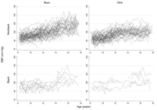
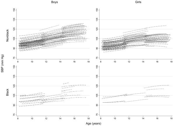
As a first step in the analysis, the data for SBP were plotted against age for each of the four race–gender groups as shown in Figure 1. In these plots, measurements for the 358 individual subjects are connected with line segments. These plots were useful in visualizing the overall patterns in the data and anticipating the analytic steps to follow. The upward trend in SBP was apparent in each group, and the vertical scatter of the data points reflects the combined variability of SBP within and between subjects. A simple two-level regression model was fitted to these data. The model was of the form

$$\begin{array}{cc}\hfill y_{\mathit{ij}}={\beta }_0+{\beta }_1\mathrm{R}+{\beta }_2\mathrm{G}+{\beta }_3\mathrm{RG}& +{\beta }_4\mathrm{A}+{\beta }_5\mathrm{RA}+{\beta }_6\mathrm{GA}+{\beta }_7\mathrm{RGA}+{\beta }_8{\mathrm{A}}^2+{\beta }_8{\mathrm{A}}^3\hfill \\ \hfill & +u_{0j}+u_{1j}\mathrm{A}+{\epsilon }_{\mathit{ij}},\hfill \end{array}$$

where y_ij is the ith measurement of SBP for the jth subject;

Figure 1.

Systolic blood pressure (SBP) versus age for four race–gender groups, Project HeartBeat! (1991–1995); for a subsample of 3152 observations on 358 subjects; SBP readings are for individuals, joined by line segments

R and G are indicator variables for race and gender (with interactions);

A is the age at measurement minus 12 years (with quadratic and cubic terms);

β's represent unknown regression coefficients;

u_0j is the random deviation in intercept and u_1j is the random deviation in the linear term for the jth subject;

ε_ij is the random deviation in the ith measurement for the jth subject;

u_0j and u_1j∼N₂(0, Ω₂), where Ω₂ is a 2 × 2 variance–covariance matrix; and

ε_ij∼N₁(0, σ_ε²), independently from u_0j and u_1j.

The first line of the model is the “fixed part” and is similar to a standard multiple regression model. The second line is the “random part” expressing random deviations at the subject level through the u terms, and at the measurement level through the ε term. An iterative method was used to find the maximum likelihood estimates of the regression coefficients β and the variances and covariances Ω₂ and σ_ε² along with their SEs.⁶ The results are presented in Table 2.

Table 2.

Estimated coefficients and p-values of a two-level model for systolic blood pressure; Project HeartBeat! (1991–1995)^a

Coefficient	Estimate	SE	p-valueb
Fixed terms
Constant	103.7	0.496	0.000
R	−1.018	1.283	0.428
G	−3.209	0.710	0.000
RG	3.772	2.309	0.102
A	2.293	0.144	0.000
RA	−0.350	0.313	0.263
GA	−0.493	0.168	0.003
RGA	0.187	0.535	0.728
A2	0.019	0.022	0.388
A3	−0.029	0.006	0.000
Between subjects
Variance (u0j)	35.245
Covariance (u0j, u1j)	1.433
Variance (u1j)	0.567
Between measurements
Variance (εij)	16.846

^aSubsample of 358 subjects

^bWald test of hypothesis that the coefficient equals zero

A, age; G, gender; R, race

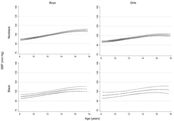
The p-values are determined by the Wald test, which compares the ratio of the coefficient estimate to its SE with the standard normal distribution. By this test, none of the terms involving R (race) is statistically different from zero at the 0.05 level, and all could be omitted from further consideration, if desired. The predicted values from the model (with all fixed terms retained), with 95% CIs, are presented in Figure 2.

Figure 2.

Predicted values with 95% CIs for systolic blood pressure (SBP) vs age in four race–gender groups, Project HeartBeat! (1991–1995), for a subsample of 358 subjects; model coefficients given in Table 2

The trends anticipated from Figure 1 were confirmed by the fitted model. Note that the width of the CIs reflect the precision with which the population average has been estimated. The difference in precision for the curves of the black and nonblack children is attributed mainly to the differing sample sizes.

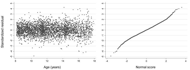
Standard residual analysis techniques were used to assess the tenability of the distributional assumptions. The plot of standardized within-subject residuals, ε_ij, against age in Figure 3 exhibited no obvious trends with age, suggesting that the Level-1 variance is constant with respect to age. The three age cohorts can be faintly discerned in this plot by noting the greater density of observations around the ages of overlap between cohorts, 11–12 and 14–15 years. The standardized within-subject residuals were also plotted against their normal scores, and the resulting nearly straight line is consistent with the assumption that ε_ij ∼N₁(0, σ_ε²).

Figure 3.

Scatter plot and normal-scores plot of within-subject residuals for systolic blood pressure (SBP) versus age, Project HeartBeat! (1991–1995), for a subsample of 3152 observations on 358 subjects

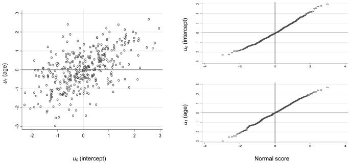
It was assumed that the distribution of the between-subject residuals u_0j for intercept and u_1j for age has the bivariate normal distribution N₂(0, Ω₂), where Ω₂ denotes the 2 × 2 variance–covariance matrix. The estimates of these residuals are plotted in Figure 4. Because the normal score plots appeared quite linear, there was no apparent contradiction to the assumption of normality.

Figure 4.

Scatter plot and normal-scores plot of between-subject residuals for systolic blood pressure (SBP) versus age, Project HeartBeat! (1991–1995), for a subsample of 358 subjects

The deviations u_0j and u_1j were added to the population predictions of Figure 2, and the result is the subject-specific predictions plotted in Figure 5. In addition to the overall trends, the pattern of the variability of the subject-specific trajectories about the population M was seen, corresponding to the subject-level random structure of the model.

Figure 5.

Subject-specific predictions of systolic blood pressure (SBP) versus age for four race–gender groups, Project HeartBeat! (1991–1995), for a subsample of 358 subjects

In summary, the cubic polynomial model described in the example appeared to provide a useful description of the SBP. Splines or other types of analyses could also have been used, but the cubic polynomial was chosen for its simplicity and its adequacy in consistently describing several different outcomes such as anthropometric measurements, blood pressures, and blood lipids.

Combining Cohorts

In an accelerated longitudinal study design with overlapping cohorts, it is assumed that each cohort is a random sample, differing only in age, from the same underlying population. Under this assumption, data from the various cohorts can be combined to estimate growth curves describing patterns of development of CVD risk factors and other parameters of interest.

To determine if this assumption was reasonable, several of the anthropometric study outcomes, including stature, weight, BMI, fat-free mass (FFM), and percent body fat (PBF), were compared between Cohorts 1 and 2 at their period of overlap (11–12 years) and between Cohorts 2 and 3 at their period of overlap (14–15 years). Regression models adjusting for age and cohort were fitted within each of the four race–gender groups and were used to make these comparisons.

To compare Cohorts 1 and 2, a multilevel model of the form

$$y_{\mathit{ij}}={\beta }_0+{\beta }_1\mathit{age}+{\beta }_2\mathrm{Cohort}2+{\beta }_3{\mathit{age}}^{\ast }\mathrm{Cohort}2+u_j+{\epsilon }_{\mathit{ij}}$$

was fitted to the data obtained from those aged between 11 and 12 years for each race–gender group. In this model, y_ij denotes the outcome variable measured on the ith occasion for the jth child. The variable age is centered at 11.5 years; Cohort2 is an indicator variable for Cohort 2; age*Cohort2 is the interaction term; u_j is a subject-level random term; and ε_ij is a measurement-level random term. In this simple multilevel model, the coefficient β₀ is the intercept, and β₁ is the slope for children in Cohort 1. For Cohort 2, the intercept is β₀+β₂, and the slope is β₁+β₃. The difference in intercepts is β₂, and the difference in slopes is β₃; thus the comparisons can be carried out by testing the hypotheses that β₂=0 and β₃=0. A similar model was fitted for comparisons of Cohorts 2 and 3.

Models for stature, weight, BMI, FFM, and PBF were fitted separately on age and cohort membership for each of the two overlapping age ranges. For this analysis, age was centered at the midpoints of each overlap period, so the difference in intercepts in Cohorts 1 and 2 was measured at 11.5 years, and the difference between Cohorts 2 and 3 was measured at 14.5 years. Results revealed only one significant difference between cohorts in intercept, and that was between Cohorts 2 and 3 for PBF (p<0.05) after adjustments for ethnicity, gender, and age (analyses not shown). There were no significant slope differences between cohorts at either point of overlap for the study variables.¹⁴

When these five outcomes were examined in the overlap periods, there were no apparent differences in the intercepts or slopes attributable to the cohorts. Thus, it was concluded that the three cohorts could be combined to estimate growth curves describing patterns of development for children aged 8–18 years.

Comparing Project HeartBeat! with U.S. Growth Data

To judge the degree to which the data obtained in Project HeartBeat! were similar to national data, the 5th, 50th, and 95th percentiles for weight, stature, and BMI by age, race, and gender from Project HeartBeat! were compared graphically with the same percentiles for U.S. children from the National Health and Nutrition Examination Survey (NHANES) I¹⁵ and NHANES II¹⁶ surveys; results are presented in Mueller et al.¹⁴

Plots of the longitudinal data confirmed that for most of the anthropometric variables and for almost every age, the distribution of the measurements was skewed upward, that is, toward the larger values. None, however, appeared multimodal except in regions of extremely sparse data. For fairly large samples, mild to moderate skewness will not appreciably affect estimation of the fixed part of the regression model used to describe the overall trajectory of change.⁶

Weight percentiles displayed graphically for Project HeartBeat! and NHANES exhibited good agreement for both nonblack boys and girls, except that for the boys, the 95th percentile of weight in Project HeartBeat! tended to exceed that for NHANES for those aged >12 years. Among the black children, there was fair agreement between Project HeartBeat! and NHANES percentiles, except for the 95th percentile, where the former was far larger. This difference may be partly attributable to instability resulting from small samples or it may be a reflection of the increased prevalence of obesity in some groups of children. A generally good agreement was seen in percentiles for stature between Project HeartBeat! and NHANES, except that curves for the former tend to be slightly higher. There was fair agreement in BMI for the nonblack children; for nonblack boys, the BMI for Project HeartBeat! tended to be slightly greater than the BMI for NHANES. For both black boys and girls, the 95th percentile for BMI in Project HeartBeat! greatly exceeded that for NHANES. This pattern was consistent with the pattern for weight.

In summary, the Project HeartBeat! and NHANES percentiles for stature were quite similar, whereas the 95th percentiles for weight and BMI in Project HeartBeat! were skewed upward, likely reflecting a secular trend toward increased obesity. Taken together, these curves, with the exceptions noted, provide evidence that the Project HeartBeat! sample is in reasonable conformity with the NHANES patterns and support the validity of inferences from the present study to the wider U.S. population of children, particularly for nonblack children. Inferences to the population of black children should be considered approximate.¹⁴

Conclusion

The accelerated longitudinal design used for Project HeartBeat! and the multilevel statistical models used for data analysis proved to be appropriate and adequate for the goals of the study. The data from the three age cohorts in Project HeartBeat! may be combined to characterize development of CVD risk factors for those aged 8–18 years, and these patterns may be generalized, with some caveats, to the U.S. population of children. No difficulties were encountered in the study design or data analysis that would suggest a different approach for similar studies in the future.

References

- 1.Labarthe DR, Nichaman MZ, Harrist RB, Grunbaum JA, Dai S. Development of cardiovascular risk factors from ages 8–18 in Project HeartBeat!: study design and patterns of change in plasma total cholesterol concentration. Circulation. 1997;95(12):2636–42. doi: 10.1161/01.cir.95.12.2636. [DOI] [PubMed] [Google Scholar]
- 2.Labarthe DR, Dai S, Day RS, et al. Project HeartBeat!: concept, development, and design. Am J Prev Med. 2009;37(1S):XXX–XXX. doi: 10.1016/j.amepre.2009.04.016. [DOI] [PMC free article] [PubMed] [Google Scholar]
- 3.Helms RW. Intentionally incomplete longitudinal designs: I. methodology and comparison of some full span designs. Stat Med. 1992;11(14–15):1889–913. doi: 10.1002/sim.4780111411. [DOI] [PubMed] [Google Scholar]
- 4.Zeger SL, Liang KY. An overview of methods for the analysis of longitudinal data. Stat Med. 1992;11(14–15):1825–39. doi: 10.1002/sim.4780111406. [DOI] [PubMed] [Google Scholar]
- 5.Rasbash J, Steele F, Browne W, Prosser B. A user's guide to MLwiN, version 2.0. University of Bristol: 2005. [Google Scholar]
- 6.Goldstein H. Multilevel statistical models. 3rd ed. Arnold Publishers; London: 2005. [Google Scholar]
- 7.Raudenbush S, Bryk A. Hierarchical linear models: applications and data analysis methods. 2nd ed. Sage Publications; Newbury Park CA: 2002. [Google Scholar]
- 8.Hox J. Multilevel analysis: techniques and applications. Earlbaum Associates; Mahwah NJ: 2002. [Google Scholar]
- 9.Snijders T, Bosker R. Multilevel analysis: an introduction to basic and advanced multilevel modeling. Sage Publications; London: 1999. [Google Scholar]
- 10.Armstrong N, Welsman JR, Nevill AM, Kirby BJ. Modeling growth and maturation changes in peak oxygen uptake in 11–13 yr olds. J Appl Physiol. 1999;87(6):2230–6. doi: 10.1152/jappl.1999.87.6.2230. [DOI] [PubMed] [Google Scholar]
- 11.Zvoch K, Stevens JJ. Successive student cohorts and longitudinal growth models: an investigation of elementary school mathematics performance. Educ Policy Anal Arch. 2006;14(2) [Google Scholar]
- 12.Black MM, Krishnakumar A. Predicting longitudinal growth curves of height and weight using ecological factors for children with and without early growth deficiency. J Nutr. 1999;129:539S–543S. doi: 10.1093/jn/129.2.539S. [DOI] [PubMed] [Google Scholar]
- 13.The European Collaborative Study. Height, weight, and growth in children born to mothers with HIV-1 infection in Europe Pediatrics. 2003;111:e52–60. doi: 10.1542/peds.111.1.e52. [DOI] [PubMed] [Google Scholar]
- 14.Mueller WH, Harrist RB, Doyle SR, Labarthe DR. Percentiles of body composition from bioelectrical impedance and body measurements in U.S. adolescents 8–17 years old: Project HeartBeat. Am J Hum Biol. 2004;16(2):135–50. doi: 10.1002/ajhb.20002. [DOI] [PubMed] [Google Scholar]
- 15.NHANES I: National Health and Nutrition Examination Survey I (1971–75) USDHHS, Public Health Service, CDC, National Center for Health Statistics; Hyattsville MA: 1981. [Google Scholar]
- 16.NHANES II: National Health and Nutrition Examination Survey II (1976–80) USDHHS, Public Health Service, CDC, National Center for Health Statistics; Hyattsville MA: 1984. [Google Scholar]