Abstract
Previous analysis of the rules regarding how much more a female should invest in a litter of size C rather than producing a litter with one more offspring revealed an invariance relationship between litter size and the range of resources per offspring in any litter size. The rule is that the range of resources per offspring should be inversely proportional to litter size. Here we present a modification of this rule that relates litter size to the total resources devoted to reproduction at that litter size. The result is that the range of resources devoted to reproduction should be the same for all litter sizes. When parental phenotypes covary linearly with resources devoted to reproduction, then those traits should also show equal ranges within each litter size category (except for litters of one). We tested this prediction by examining the range in body size (=total length) of female mosquito fish (Gambusia hubbsi) at different litter sizes. Because resources devoted to reproduction may take many forms (e.g., nest defense), this prediction may have broad applicability.
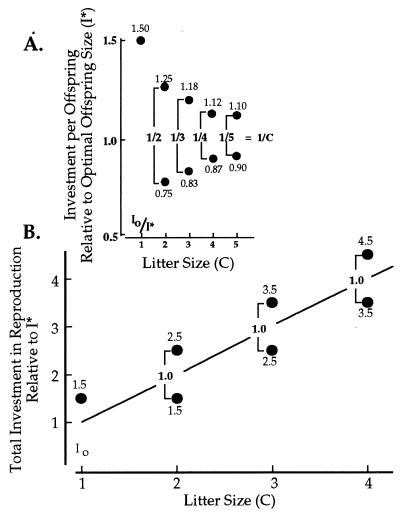
A classic problem in life history theory involves the trade-off between resources per offspring and number of offspring (1–4). The general solution to this problem is to provision each offspring with that amount of resource that maximizes offspring survivorship relative to investment per offspring (2). At small litter sizes females are confronted with the problem of whether to produce, say, one offspring of larger than optimal size or two offspring of smaller than optimal size. As a solution to this question, it is clear that a female should continue to invest in offspring in the smaller litter, but only up to the point where the fitness of a litter of size C is equal to the fitness of a litter of size C+1. That is, there should be a range of offspring sizes associated with any litter size. And, as we have shown (5), when the range of resources per individual offspring in any litter size is scaled to optimal offspring size (I*), it is inversely equal to litter size (Fig. 1A). We found that this rule was invariant (5, 6) over an exceptionally broad range of functions relating survivorship to investment per offspring. That is, the predicted range of resources was independent of the shape of the underlying trade-off function.
Figure 1.
Ranges in investment per offspring (A) and total investment (B) in litters with different numbers of offspring relative to the optimal investment per offspring (I*). Io is the size of the smallest viable offspring. The numbers within each figure refer to the upper and lower limits for investment in litters of different sizes (from ref. 5). The numbers between brackets are the ranges in offspring size. In A, the range is inversely proportional to litter size (C). In B, the range is constant when A is scaled to total investment in reproduction.
Few published data are available to test this hypothesis because the range in investment per offspring is greatest at small litter size and decreases with increased litter size (7, 8). As a consequence, this prediction is difficult to test at larger (>5) litter sizes. Experimental provisioning of females may allow determination of resource levels required to shift litter size from C to C+1, and the range of resources over which a litter of size C prevails; however, this may be logistically difficult. Here we provide and test a litter size independent alternative formulation of that result. We suggest that this alternative may have applicability over a broad range of problems in evolutionary ecology.
If we consider the total resources (R) devoted to offspring at any litter size (C), rather than the contribution to each individual offspring, then the total resources for any litter are CI, where I is offspring size. If Imax and Imin are the largest- and smallest-sized offspring associated with any litter size C, then, as we showed (5), Imax − Imin is proportional to C−1 and thus
 |
When offspring size is measured relative to optimal offspring size, I*, then, to a good approximation (5), Imax/I* − Imin/I* = C−1 and
 |
That is, the total resources increase linearly with litter size, but the range in resources per litter is constant and invariant with litter size.
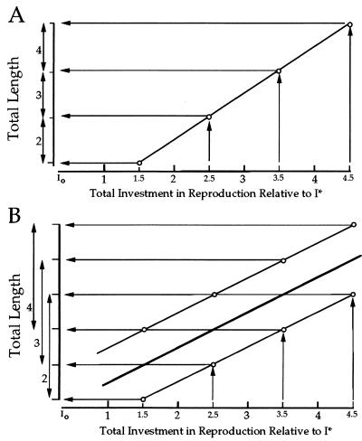
Although it is not difficult to measure litter size, determining the resources devoted to reproduction often is imprecise or impractical (e.g., measuring the cost of parental care). However, it is often the case that litter size is correlated with a phenotypic trait(s) of the parent. If we assume that R bears a linear relationship to that trait, and all offspring within litters are of equal average size, then it follows that the range in that phenotypic trait should be equal over all litter sizes (Fig. 2A). For example, body size often is correlated with litter size such that larger females produce larger litters. Provided that relationship is linear and average offspring size does not change with litter size, then the range in female body size should be the same for all litter sizes (Fig. 2B).
Figure 2.
If resources devoted to reproduction scale linearly with body size (total length) such that each increment in length results in a corresponding increase in allocation of resources to reproduction, then the ranges in total length will be the same in all litter size classes and nonoverlapping (as shown to the left of the abscissa in A). Although such cases may occur, it is more likely that the resources devoted to reproduction is variable among females of the same total length. Such variation may be caused by age, previous reproductive activity, or recent foraging success. Provided the regression of total length on the resources devoted to reproduction is linear (the heavy line in B), the expectation of equal ranges would still hold, although the ranges would overlap (as shown to the left of the abscissa in B).
Gambusia hubbsi is an endemic mosquito fish from the Bahamas. It is a live-bearer producing large yolky eggs. Eggs within litters are uniform in size, and maximum egg sizes in litters from two to six correspond to the predicted maxima illustrated in Fig. 1A (7). In other poeciliids studied so far, egg size approximates neonate size (9). In only 3 of the 33 populations where we have samples great enough to test for a correlation between litter size and egg size was there a significant correlation (P < 0.05). In two instances it was positive; in one it was negative. Overall, 18 of the correlations were positive, and 15 were negative. Thus, egg size does not change in any consistent way with litter size within populations. However, egg size does differ among populations, as does mean litter size and female total length (cf. Table 1).
Table 1.
Means and ranges in total length (T.L.) of female Gambusia hubbsi that produced litters of different sizes in different populations on Andros, Bahamas (see ref. 10 for locations)
| Location (egg vol., ne) N (SEM) b* | Litter size
|
Difference in ranges | P† | |||||
|---|---|---|---|---|---|---|---|---|
| 2 | 3 | 4 | 5 | 6 | ||||
| Ken’s (8.9, 34) | n | 33 | 7 | |||||
| 95 (0.28) | T.L. | 28.1 | 30.2 | |||||
| 2.59 | Range | 8 (23–31) | 8 (26–34) | 0 | 0.915 | |||
| BD (4.2, 4) | n | 12 | 9 | |||||
| 33 (0.60) | T.L. | 25.8 | 26.89 | |||||
| 1.76 | Range | 9 (6.57) | 9 (8.11) | 0 | 0.781 | |||
| ETL (7.7, 14) | n | 6 | 6 | 6 | ||||
| 24 (0.94) | T.L. | 33.7 | 34.7 | 40.7 | ||||
| 1.77 | Range | 7 (31–38) | 5 (32–37) | 5 (38–43) | 2 | 0.606 | ||
| MB (6.2, 6) | n | 8 | 5 | 5 | ||||
| 23 (0.59) | T.L. | 32.4 | 34.2 | 35.4 | ||||
| 1.78 | Range | 6 (30–36) | 8 (31–39) | 6 (33–39) | 2 | 0.465 | ||
| Airport (5.7, 25) | n | 24 | 22 | 11 | 9 | |||
| 79 (0.39) | T.L. | 24.8 | 27.8 | 29.6 | 30.1 | |||
| 1.52 | Range | 7 (22–29) | 8 (24–32) | 5 (27–32) | 5 (28–33) | 3 | 0.460 | |
| Last Ditch (4.7, 28) | n | 17 | 10 | 6 | 6 | |||
| 56 (0.64) | T.L. | 25.1 | 27.9 | 31.2 | 32.2 | |||
| 1.66 | Range | 8 (22–30) | 11 (25–36) | 10 (28–37) | 11 (28–39) | 3 | 0.539 | |
| Runway (4.8, 17) | n | 8 | 19 | 14 | 7 | |||
| 55 (0.44) | T.L. | 25.6 | 28.0 | 28.0 | 31.3 | |||
| 1.49 | Range | 5 (24–29) | 10 (23–33) | 9 (23–32) | 11 (25–36) | 6 | 0.291 | |
| J’s (9.7, 32) | n | 11 | 10 | 13 | 12 | 8 | ||
| 63 (0.49) | T.L. | 33.0 | 33.2 | 34.5 | 35.8 | 35.0 | ||
| 0.80 | Range | 8 (29–37) | 14 (25–39) | 9 (29–38) | 9 (32–41) | 4 (33–37) | 10 | 0.030 |
| Lime Pond (3.0, 17) | n | 17 | 15 | 11 | 5 | |||
| 55 (0.30) | T.L. | 23.5 | 23.8 | 25.5 | 27.6 | |||
| 1.11 | Range | 6 (21–27) | 6 (21–27) | 6 (24–30) | 7 (25–32) | 1 | 0.600 | |
| NG2 (7.3, 25) | n | 6 | 7 | 6 | 16 | |||
| 54 (0.45) | T.L. | 29.8 | 33.0 | 33.3 | 34.1 | |||
| 0.86 | Range | 4 (28–32) | 4 (31–35) | 6 (31–37) | 8 (30–38) | 4 | 0.242 | |
Only litter sizes with n values of five or greater are included. Litters of one are excluded from the test for equality of ranges because the model makes no prediction regarding the range in litters of that size. ne, is the sample size for egg volumes.
Slope of T.L. on litter size.
P is the probability of observing a range difference greater than that found in each population. Because there are no tests for equality of ranges, these probabilities were determined through a randomization program (11). Random subsamples were drawn from the total sample of females (N) in each locality. The number in each subsample corresponded to the number of females (n) in those litter size classes with the greatest difference in range. The mean of each subsample was calculated and compared with the observed subsample mean. If the calculated means fell within the confidence limits set for those means (±1.96 times SEM for the population), the difference in the ranges of the two subsamples was compared to the observed difference in the range. The proportion of ranges greater than the observed difference is based on 1,000 iterations.
Within our populations, female total length and litter size are highly correlated (Table 1, and ref. 10). The slope of the regression of total length on litter size ranges from 0.7 mm/offspring to 3.6 mm/offspring among populations. In 33 of 36 populations the relationship between litter size and egg size is linear. The three populations in which relationship is curvilinear are excluded from this analysis.
The range in female total length is the same over all litters in eight of the nine populations for which we have sample sizes large enough to test for heterogeneity of ranges (Table 1). Because we are comparing the most extreme ranges within any population, our test is biased toward rejection of the hypothesis of equality of ranges. In one population (J’s), females that produced litters of two and six have notably larger and smaller ranges in total length than we found in other litter classes. Even with this exception the ranges in total length are remarkably uniform over litter sizes within localities.
The probability of observing a range difference greater than observed varied from 0.92 to 0.03 (Table 1), and the variation in probabilities and range differences, relative to the slope of total length on litter size, is informative in the following way. If the slope of total length on litter size is shallow, then all litter size classes have similar means. Although we expect the observed ranges to be identical, the similarity among ranges should be high under any circumstance. When the slope is steep, the difference between means increases and greater differences in ranges due to chance should be more common. That is, if the uniformity we observe is due to chance, then both the difference between ranges and the probability of observing a greater difference (holding the range difference constant) should increase with the slope.
Among our populations the probability of observing a greater difference increases as the slope increases (holding the range difference constant, partial r = 0.78, P < 0.05); by contrast, the difference between ranges decreases significantly as the slope increases (r = −0.77, P < 0.05, Table 1). The first correlation is to be expected if range similarities are largely due to chance, whereas the second is not. It is, however, consistent with the hypothesis that the observed ranges are uniform over different litter sizes.
Gambusia populations on Andros that we have studied are isolated from one another and occupy a wide range of habitats (10); as a result, females in different populations may apportion resources for reproduction differently. If so, the prediction that the range in female total length within any litter size (except litters of one) should be the same over all litters stills holds true, even though the underlying fitness function may differ among populations.
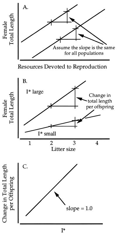
If females in all localities apportion resources for reproduction in the same linear fashion with regard to total length [i.e., the slopes of the relationship between total length and resources devoted to reproduction are the same (Fig. 3A)], then in populations where females produce larger eggs, each additional egg will require absolutely more resource. If we assume there is an optimal egg volume (I*) associated with the ecological conditions of each locality, then the increment in total length associated with each additional egg should be greater in populations where I* is larger, and correspondingly the increment in total length per egg will be less where I* is smaller (Fig. 3B). If these conditions are met, differences in the slope of total length on litter number among populations are proportional to the difference in resources needed to produce an additional offspring. Assuming differences in egg volume estimate differences in I* among populations, the relationship between slope of total length on litter number and egg volume across populations should be positive. If the allocation of resources to reproduction is similar (i.e., has the same slope) among populations (Fig. 3A), then we expect the slope to be directly proportional to egg volume, that is, the slope of the log-transformed data = 1.0 (Fig. 3C).
Figure 3.
(A) The relationship between total length, and allocation of resources for reproduction in different populations. (B) Differences in optimal offspring size (I*) in different environments alter the relationship between female total length and litter size. (C) The expected relationship between the change total length relative to litter size and optimal offspring size provided the slopes in A are the same. See text for further discussion.
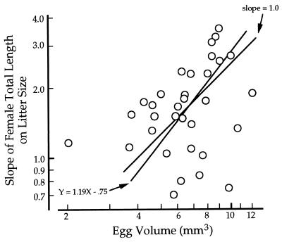
Egg volume varies among populations of G. hubbsi as does the slope of total length on litter size. Slopes vary by half an order of magnitude (0.7–3.6 mm/egg) among the 36 populations we have studied, and there is a 6-fold difference in egg volume (2.0–12.7 mm3, Fig. 4). Because both mean egg volume and the slope of total length on litter size are estimated with error, we used a major axis regression to analyze the relationship between these two variables. The relation is significant (P < 0.05) and the estimated slope (1.19, 95% confidence limits = ±0.495) is not different from 1.0 (P < 0.50, Fig. 4). Although the proportion of variation explained by the regression is small, the observed linearity and slope are consistent with the idea that even though egg size, female total length, and the slope of total length on litter size vary among populations, the underlying allocation rule does not.
Figure 4.
Major axis regression of Log egg volume on Log slope of female total length on litter size (r2 = 0.103, P < 0.05) for 33 populations of G. hubbsi from Andros, Bahamas. Confidence limits, estimated of significance and comparison of the observed slope to an expected slope of 1.0, were determined by use of standard randomization methods (11). Here, random pairings (5,000 iterations) of egg volume with the slope of total length on litter size yielded 95% confidence limits of ±0.495 for the slope of the major axis regression. If the expected slope is 1.0, a slope that is more extreme than 1.19 is expected to occur 53.7% of the time.
The question of optimal investment in offspring at small litter number is only one of a suite of problems that involve an integer threshold effect (12–14), which we term here “integer-change-over problems.” Here we have explored the rules associated with how much more a female should invest in a litter of C offspring before her fitness is enhanced by investing in C+1 offspring. To test those rules we have used female total length as a surrogate for resources. By doing so we believe that we have made testing of the model more tractable. But there are other integer-change-over problems in which the nature of that investment may take different forms, and transformation of resources used for reproduction into some other, more easily measured form may allow for testing of hypotheses regarding how resources actually are allocated. In Table 2 we have summarized some situations that have occurred to us. However, it is unclear whether analogous rules underlie these integer-change-over problems—rules such as going from C to C+1. If they do, then equality of ranges at each integer class may be viewed appropriately as indicative of those analogies. Lloyd (13), in particular, has noted the similarities between optimality models dealing with “packaging strategies” for size and number of repeating units (progeny, flower number, etc.) and models in which time is a surrogate for reproductive fitness (12, 14). We include Table 2 in hopes of stimulating other workers to examine these (and other) integer-change-over problems for equality of ranges within integer classes both theoretically and empirically.
Table 2.
Circumstances in which an integer-change-over problem exists and where equality of ranges may occur
| Resource | Equality of ranges in |
|---|---|
| Resources for reproduction are a function of egg size. Egg number increases linearly with female total length. Egg size is uncorrelated with egg number. | Female total length within litter sizes (this study) |
| Females provision offspring. Egg sizes equal across clutch size. Feeding rates increase with clutch size. | Feeding rates within each clutch size |
| Females provision offspring by placing eggs on patches of resource (e.g., parasitoids). Patches vary in quality, and the number of eggs per patch increases linearly with patch richness. | Patch characteristics across patches with different numbers of eggs |
| Females are aided in reproduction by other individuals (e.g., cooperatively breeding birds). Eggs are of equal size, and larger clutches have more helpers. | Number of helpers associated with each clutch size |
| Females leave eggs with another individual (male) who provides parental care. Survivorship of offspring is correlated with phenotypic traits of the care giver (e.g., size), and males with enhanced traits attract more females. | Phenotypic traits associated with parental care among males with equal numbers of matings |
| Females mate with males who enhance offspring survival indirectly (e.g., “good genes”). Males signal differences in quality. Males with enhanced “signals” attract more females. | Phenotypic traits serving as signals among males with equal numbers of matings |
Acknowledgments
We thank L. Brown and M. Matsui for their help with all aspects of this study and G. C. Williams for comments on the manuscript. The Ministry of Agriculture and Fisheries gave us permission to study G. hubbsi populations on Andros. This work was supported by the Biology Department of the University of Utah, Earthwatch, and the National Geographic Society. An anonymous reviewer suggested the we develop randomization procedures to test for equality of ranges and to evaluate the major axis regression.
Footnotes
This paper was submitted directly (Track II) to the Proceedings Office.
References
- 1.Schaffer W M, Gadgil M. In: Ecology and Evolution of Communities. Cody M, Diamond J A, editors. Cambridge, MA: Harvard Univ. Press; 1975. pp. 142–157. [Google Scholar]
- 2.Smith C C, Fretwell S D. Am Nat. 1974;108:499–506. [Google Scholar]
- 3.Stearns S C. The Evolution of Life Histories. Oxford: Oxford Univ. Press; 1992. [Google Scholar]
- 4.Wooton R J. J Fish Biol. 1994;45:1067–1077. [Google Scholar]
- 5.Charnov E L, Downhower J F. Nature (London) 1995;376:418–419. doi: 10.1038/376418a0. [DOI] [PubMed] [Google Scholar]
- 6.Charnov E L. Life History Invariants. Oxford: Oxford Univ. Press; 1993. [Google Scholar]
- 7.Charnov E L, Downhower J F, Brown L. Evol Ecol. 1995;9:57–63. [Google Scholar]
- 8.Ebert D. Ecology. 1994;75:568–571. [Google Scholar]
- 9.Schrimshaw N S. Biol Bull. 1945;88:233–246. [Google Scholar]
- 10.Brown L, Downhower J F. Bahamas Nat. 1993;7:1–10. [Google Scholar]
- 11.Manly B F J. Randomization, Bootstrap and Monte Carlo Methods in Biology. 2nd Ed. New York: Chapman & Hall; 1997. [Google Scholar]
- 12.Charnov E L. Theor Pop Biol. 1976;9:129–136. doi: 10.1016/0040-5809(76)90040-x. [DOI] [PubMed] [Google Scholar]
- 13.Lloyd D G. Am Nat. 1987;129:800–817. [Google Scholar]
- 14.Krebs J R, McCleery R H. In: Behavioral Ecology. 2nd Ed. Krebs J R, Davies N K, editors. Oxford: Blackwell; 1984. pp. 91–121. [Google Scholar]


