Defining Coarse-Grained Representations of Large Biomolecules and Biomolecular Complexes from Elastic Network Models

Abstract

Coarse-grained (CG) models of large biomolecular complexes enable simulations of these systems over long timescales that are not accessible for atomistic molecular dynamics (MD) simulations. A systematic methodology, called essential dynamics coarse-graining (ED-CG), has been developed for defining coarse-grained sites in a large biomolecule. The method variationally determines the CG sites so that key dynamic domains in the protein are preserved in the CG representation. The original ED-CG method relies on a principal component analysis (PCA) of a MD trajectory. However, for many large proteins and multi-protein complexes such an analysis may not converge or even be possible. This work develops a new ED-CG scheme using an elastic network model (ENM) of the protein structure. In this procedure, the low-frequency normal modes obtained by ENM are used to define dynamic domains and to define the CG representation accordingly. The method is then applied to several proteins, such as the HIV-1 CA protein dimer, ATP-bound G-actin, and the Arp2/3 complex. Numerical results show that ED-CG with ENM (ENM-ED-CG) is much faster than ED-CG with PCA because no MD is necessary. The ENM-ED-CG models also capture functional essential dynamics of the proteins almost as well as those using full MD with PCA. Therefore, the ENM-ED-CG method may be better suited to coarse-grain a very large biomolecule or biomolecular complex that is too computationally expensive to be simulated by conventional MD, or when a high resolution atomic structure is not even available.

Introduction

Coarse-grained (CG) models of complex biomolecules enable one to simulate large biological systems over longer effective timescales than atomistic molecular dynamics (MD) simulations (1). Therefore various CG approaches have been developed with rapidly growing interest, according to different principles (2–4). Generally speaking, a CG model is defined by reducing the large number of degrees of freedom in a biomolecule into a significantly smaller set of CG sites. Once the number of CG sites for a given system has been determined, an important consideration is where to place them, i.e., how to establish a reasonable mapping between the atomistic and CG levels of resolution.

Among different CG methodologies, elastic network models (ENMs) have attracted considerable interest (5–11). In a typical ENM, each residue is represented by one CG site (usually located at the position of its C_α atom). The interactions between C_α atoms that are within a cutoff distance are harmonic (spring potentials), and the spring constants in the network can be uniform (5) or heterogeneous (12,13). ENMs have proven to be very popular because of the following advantages. They are simple to implement and only a single structure is needed (7). They can provide valuable information on functional dynamics of a large biomolecule or biomolecular complex without computationally-expensive MD data (14–17). They can also be fruitfully used to fit cryo-electron microscopy (cryo-EM) data (18–20).

An implicit feature of most ENMs is that all of the atoms in each residue are mapped onto the position of each C_α atom. However, in some cases a CG model with a resolution lower than ENM (typical one site per residue) is needed for a large biomolecule (21–25). Beyond the resolution of individual residues, it becomes increasingly difficult to choose a CG mapping based on intuition alone. We have addressed this challenge previously by developing a systematic and quantitative methodology to define a relatively small number of CG sites for a large biomolecule, called essential dynamics coarse-graining (ED-CG) (26). In particular, this approach variationally determines a CG representation that preserves the important functional dynamics (the so-called essential dynamics (27)) of the biomolecule. In Zhang et al. (26), the essential dynamics of the biomolecule were characterized by principal component analysis (PCA) of an atomistic MD trajectory (27–29).

This study introduces what we believe to be a new ED-CG scheme using an ENM. Instead of a PCA derived from a computationally expensive and potentially even infeasible MD trajectory, the low-frequency normal modes calculated by ENM are used to characterize the functional essential dynamics of the system. Therefore the CG mapping can be defined quickly from a single structure of the biomolecule without carrying out an MD simulation and PCA analysis. We anticipate that this approach, denoted ENM-ED-CG, will be of significant use and will also help to provide key insight into functionally important domains of proteins and multi-protein complexes, especially in terms of their primary amino acid sequences.

In the subsequent sections, an ENM, also called an anisotropic network model (6), will be reviewed, followed by the ENM-ED-CG development. There is also a different theoretical underpinning when using ENM instead of PCA for ED-CG. The resulting method is then applied to several proteins. The first two are the HIV-1 CA protein dimer and ATP-bound globular actin (G-actin), and the results are compared with the ED-CG models developed using MD with PCA. The third application is the actin-related protein (Arp) 2/3 complex in both the inactive and active states, which is the first time ED-CG is carried out for such a large multi-protein complex. Concluding remarks are provided to summarize this work.

Theory and Methods

ENM

In our method, an ENM called an anisotropic network model (6), is used because protein fluctuations are generally anisotropic (30–32). Both the direction of the collective motion as well as its magnitude is important to consider as each has been related to protein function. Frequently in this approach, only the positions of C_α atoms are used. There is, however, no inherent restriction on the number of CG sites or the number of atoms or residues they represent. The harmonic potential of the elastic network can be written as

$$V=\sum _{\text{i,}\text{j}>\text{i}}\frac{1}{2}{k}_{\text{ij}}\Delta r_{\text{ij}}^2\text{.}$$ (1)

Here, $\Delta r_{\text{ij}}=r_{\text{ij}}-r_{\text{ij}}^0$ is the fluctuation between atoms i and j, where $r_{\text{ij}}^0$ is their equilibrium distance, and k_ij is spring constant, which is given by

$$k_{\text{ij}}=\{\begin{array}{c}cif{r}_{\text{ij}}\le r_{\text{cs}}\\ {10}^{-2}cif{r}_{\text{cs}}<r_{\text{ij}}\le r_{\text{cm}}\\ {10}^{-4}cif{r}_{\text{cm}}<r_{\text{ij}}\le r_{\text{cl}}\\ 0if{r}_{\text{ij}}>r_{\text{cl}}\end{array},$$ (2)

where c is a constant. There are three cut-off distances, which are used to model interactions from strong to weak. The parameter r_cs is the short cut-off distance of the first interaction shell, and r_cm and r_cl are the middle and long cut-off distances, respectively. Thus, the heterogeneous ENM approximates a wide range of interactions in the atomistic model. In this article, the three cut-off distances were taken as 7, 11, and 15 Å, respectively.

In the case of n atoms, the position of atom i is r_i, with components denoted by $r_{i_x}$ x = 1,2,3. The second derivatives of the overall potential (Eq. 1) can be organized in a Hessian matrix $\mathbf{H}\in {\mathbb{R}}^{3\text{n}}\times {\mathbb{R}}^{3\text{n}}$

$$\mathbf{H}=\left[\begin{array}{cccc}{\mathbf{h}}_{11}& {\mathbf{h}}_{12}& \cdots & {\mathbf{h}}_{1\text{n}}\\ {\mathbf{h}}_{21}& {\mathbf{h}}_{22}& \cdots & {\mathbf{h}}_{2\text{n}}\\ ⋮& & & ⋮\\ {\mathbf{h}}_{\text{n}1}& {\mathbf{h}}_{\text{n}2}& \cdots & {\mathbf{h}}_{\text{nn}}\end{array}\right]\text{.}$$ (3)

The term ${\mathbf{h}}_{\text{ij}}\in {\mathbb{R}}^3\times {\mathbb{R}}^3$ is a super-element in H. The off-diagonal super-elements (i ≠ j) are given by

$${\mathbf{h}}_{\text{ij}}=\left[\begin{array}{ccc}{\partial }^{2}V/\partial r_{{\text{i}}_{\text{1}}}\partial r_{{\text{j}}_{\text{1}}}& {\partial }^{2}V/\partial r_{{\text{i}}_{\text{1}}}\partial r_{{\text{j}}_{\text{2}}}& {\partial }^{2}V/\partial r_{i_1}\partial r_{{\text{j}}_{\text{3}}}\\ {\partial }^{2}V/\partial r_{{\text{i}}_{\text{2}}}\partial r_{{\text{j}}_{\text{1}}}& {\partial }^{2}V/\partial r_{{\text{i}}_{\text{2}}}\partial r_{{\text{j}}_{\text{2}}}& {\partial }^{2}V/\partial r_{i_2}\partial r_{{\text{j}}_{\text{3}}}\\ {\partial }^{2}V/\partial r_{{\text{i}}_{\text{3}}}\partial r_{{\text{j}}_{\text{1}}}& {\partial }^{2}V/\partial r_{{\text{i}}_{\text{3}}}\partial r_{{\text{j}}_{\text{2}}}& {\partial }^{2}V/\partial r_{i_3}\partial r_{{\text{j}}_{\text{3}}}\end{array}\right],$$ (4)

where

$${\partial }^{2}V/\partial r_{{\text{i}}_{\text{x}}}\partial r_{{\text{j}}_{\text{y}}}=-k_{\text{ij}}\frac{\left(r_{{\text{j}}_{\text{x}}}-r_{{\text{i}}_{\text{x}}}\right)\left(r_{{\text{j}}_{\text{y}}}-r_{{\text{i}}_{\text{y}}}\right)}{r_{\text{ij}}^2}{|}_{r_{\text{ij}}=r_{\text{ij}}^0}\text{.}$$ (5)

The diagonal super-elements (i = j) are given by

$${\mathbf{h}}_{\text{ii}}=\left[\begin{array}{ccc}{\partial }^{2}V/\partial r_{{\text{i}}_{\text{1}}}^2& {\partial }^{2}V/\partial r_{{\text{i}}_{\text{1}}}\partial r_{{\text{i}}_{\text{2}}}& {\partial }^{2}V/\partial r_{{\text{i}}_{\text{1}}}\partial r_{{\text{i}}_{\text{3}}}\\ {\partial }^{2}V/\partial r_{{\text{i}}_{\text{2}}}\partial r_{{\text{i}}_{\text{1}}}& {\partial }^{2}V/\partial r_{{\text{i}}_{\text{2}}}^2& {\partial }^{2}V/\partial r_{{\text{i}}_{\text{2}}}\partial r_{{\text{i}}_{\text{3}}}\\ {\partial }^{2}V/\partial r_{{\text{i}}_{\text{3}}}\partial r_{{\text{i}}_{\text{1}}}& {\partial }^{2}V/\partial r_{{\text{i}}_{\text{3}}}\partial r_{{\text{i}}_{\text{2}}}& {\partial }^{2}V/\partial r_{{\text{i}}_{\text{3}}}^{\text{2}}\end{array}\right],$$ (6)

where

$${\partial }^{2}V/\partial r_{{\text{i}}_{\text{x}}}\partial r_{{\text{i}}_{\text{y}}}=\sum _{\text{j}\ne \text{i}}{k}_{\text{ij}}\frac{\left(r_{{\text{j}}_{\text{x}}}-r_{{\text{i}}_{\text{x}}}\right)\left(r_{{\text{j}}_{\text{y}}}-r_{{\text{i}}_{\text{y}}}\right)}{r_{\text{ij}}^{\text{2}}}{|}_{r_{\text{ij}}=r_{\text{ij}}^0}\text{.}$$ (7)

The Hessian matrix H (Eq. 3) can be diagonalized to yield a matrix of eigenvectors and corresponding eigenvalues

$$H\left(i_{\text{x}},j_{\text{y}}\right)=\sum _{\text{q}=1}^{3\text{n}}{\Psi }_{\text{q}}^{{\text{i}}_{\text{x}}}{\lambda }_{\text{q}}{\Psi }_{\text{q}}^{{\text{j}}_{\text{y}}}\text{.}$$ (8)

Here ${\Psi }_{\text{q}}^{{\text{i}}_{\text{x}}}$ and ${\Psi }_{\text{q}}^{{\text{j}}_{\text{y}}}$ are two components corresponding to the x (=1, 2, 3) coordinate of atom i and the y (=1, 2, 3) coordinate of atom j, respectively, in the eigenvector ${\Psi }_{\text{q}}\in {\mathbb{R}}^{3\text{n}}$ (normal mode), which is the q^th column of the matrix $\Psi \in {\mathbb{R}}^{\text{3n}}\times {\mathbb{R}}^{\text{3n}}$. There are 3n eigenvalues λ_q in total, of which the first six are zero because they are associated with the overall translations and rotations of the system. It should be noted here that a relatively long cut-off (r_d = 15 Å) was used to avoid more than six zero eigenvalues (6). Each nonzero eigenvalue and corresponding eigenvector reflects the normal mode frequency and Cartesian components of this mode, respectively. Different choices of the constant c (Eq. 2) will only change the eigenvalues, but not the eigenvectors. Many studies have indicated the first few low-frequency normal modes represent functionally important motions in biomolecules, which is further discussed in two reviews (28,29).

The ENM-ED-CG method

The details of the ED-CG methodology are described in Zhang et al. (26). The original ED-CG used the essential PCA modes of a MD trajectory to systematically define CG sites in a protein from its primary amino acid sequence. The atoms that move together in a highly correlated fashion (a dynamic domain) are mapped into a CG site by minimizing the residual

$${\chi }^2=\frac{1}{3N}\sum _{\text{I}=1}^{\text{N}}\frac{1}{n_{\text{t}}}\sum _{\text{t=1}}^{{\text{n}}_{\text{t}}}\left(\sum _{\text{i}\in \text{I}}\sum _{\text{j}\ge \text{i}\in \text{I}}{\left|\Delta {\mathbf{r}}_{\text{i}}^{\text{ED}}\left(t\right)-\Delta {\mathbf{r}}_{\text{j}}^{\text{ED}}\left(t\right)\right|}^2\right),$$ (9)

where N is the number of CG sites, n_t is the number of configurations in the MD trajectory, and $\Delta {\mathbf{r}}_{\text{i}}^{\text{ED}}\left(t\right)$ is the fluctuation of atom i in the essential subspace at time t. If another atom j moves together with the atom i, the fluctuation difference between them, ${\left|\Delta r_{\text{i}}^{\text{ED}}\left(t\right)-\Delta r_{\text{j}}^{\text{ED}}\left(t\right)\right|}^2$, will be very small. Thus the two atoms should be grouped into the same CG site I. A CG model defined by this algorithm can preserve dynamic domains, and therefore approximate the functional essential dynamics of the biomolecule at the CG level.

In the case of an ENM, there is only a single structure of the protein. Therefore, Eq. 9 can be rewritten as

$${\chi }^2=\frac{1}{3N}\sum _{\text{I}=1}^{\text{N}}\sum _{\text{i}\in \text{I}}\sum _{\text{j}\ge \text{i}\in \text{I}}\langle {\left(\Delta {\mathbf{r}}_{\text{i}}^{\text{ED}}\right)}^2-2\Delta {\mathbf{r}}_{\text{i}}^{\text{ED}}\cdot \Delta {\mathbf{r}}_{\text{j}}^{\text{ED}}+{\left(\Delta {\mathbf{r}}_{\text{j}}^{\text{ED}}\right)}^2\rangle ,$$ (10)

where $\langle {\left(\Delta {\mathbf{r}}_{\text{i}}^{\text{ED}}\right)}^2\rangle$ is the mean-square fluctuation of atom i in the essential subspace. According to the classical theory of networks (33),

$$\langle {\left(\Delta {\mathbf{r}}_{\text{i}}\right)}^2\rangle =k_{\text{B}}T\text{t}\text{r}\left[{\mathbf{h}}_{\text{ii}}^{-1}\right],$$ (11)

where k_B is the Boltzmann constant, and T is the absolute temperature. The term ${\mathbf{h}}_{\text{ii}}^{-1}\in {\mathbb{R}}^3\times {\mathbb{R}}^3$ is the i^th super-element of the inverse matrix of H $\left({\mathbf{H}}^{-1}\in {\mathbb{R}}^{\text{3n}}\times {\mathbb{R}}^{\text{3n}}\right)$, and $\text{t}\text{r}\left[{\mathbf{h}}_{\text{ii}}^{-1}\right]$ refers to the trace of this 3 × 3 matrix, i.e.,

$$\mathrm{tr}\left[{\mathbf{h}}_{\text{ii}}^{-1}\right]=\sum _{\text{x}=1}^3\sum _{\text{q}=7}^{3\text{n}}{\Psi }_{\text{q}}^{{\text{i}}_{\text{x}}}{\lambda }_{\text{q}}^{-1}{\Psi }_{\text{q}}^{{\text{i}}_{\text{x}}}\text{.}$$ (12)

As in PCA an essential subspace is defined, which consists of the first n_ED of the normal modes with nonzero eigenvalues obtained by the ENM. In practice, n_ED = 3N − 6 because an N-site CG model has 3N − 6 internal degrees of freedom. In this essential subspace, $\text{t}\text{r}\left[{\left({\mathbf{h}}^{\text{ED}}\right)}_{\text{ii}}^{-1}\right]=\sum _{\text{x}=1}^3\sum _{\text{q}=7}^{{\text{n}}_{\text{ED}}+6}{\Psi }_{\text{q}}^{{\text{i}}_{\text{x}}}{\lambda }_{\text{q}}^{-1}{\Psi }_{\text{q}}^{{\text{i}}_{\text{x}}}$, and then

$$\langle {\left(\Delta {\mathbf{r}}_{\text{i}}^{\text{ED}}\right)}^2\rangle =k_{\text{B}}T\text{t}\text{r}\left[{\left({\mathbf{h}}^{\text{ED}}\right)}_{\text{ii}}^{-1}\right]\text{.}$$ (13)

It follows that Eq. 10 may be recast in the following form:

$${\chi }^2=\frac{k_{\text{B}}T}{3N}\sum _{\text{I}=1}^{\text{N}}\sum _{\text{i}\in \text{I}}\sum _{\text{j}\ge \text{i}\in \text{I}}\left(\text{t}\text{r}\left[{\left({\mathbf{h}}^{\text{ED}}\right)}_{\text{ii}}^{-1}\right]-2\text{t}\text{r}\left[{\left({\mathbf{h}}^{\text{ED}}\right)}_{\text{ij}}^{-1}\right]+\text{t}\text{r}\left[{\left({\mathbf{h}}^{\text{ED}}\right)}_{\text{jj}}^{-1}\right]\right)\text{.}$$ (14)

Different choices of the constant c will only change the absolute values of the residual (Eq. 14), but will not affect the final ENM-ED-CG results.

In this study, the same numerical algorithms as in Zhang et al. (26) are used to minimize the residual (Eq. 14) to obtain the best CG model that reflects the low-frequency functional dynamics characterized by the ENM. If one wants to place N CG sites in a protein, the same number of dynamic domains will be determined first. These domains are assumed to be contiguous on the primary sequence, so they can be chosen by determining N-1 boundary atoms (the last atom in each domain) that partition the primary sequence of the protein. Initially the N-1 boundary atoms (called a boundary-atom set) are located along the primary sequence randomly, then the residual (Eq. 14) is minimized by variationally adjusting the locations of these boundary atoms, using a global simulated annealing (34) followed by a local steepest descent search. After the boundary-atom set with the minimum residual is determined, the center-of-mass of each dynamic domain is chosen as a CG site. In this way the optimal partitioning of the primary sequence into CG sites is determined, and the resulting CG model may in principle explore conformational space while keeping the underlying protein primary sequence intact.

Results and Discussion

The HIV-1 CA protein dimer and ATP-bound G-actin

We have previously used the ED-CG scheme with PCA of atomistic MD trajectories to obtain ED-CG models for the HIV-1 CA dimer and ATP-bound G-actin (26). Herein CG models of these two systems are also built by ENM-ED-CG of a single structure to compare with those obtained from MD with PCA.

The HIV-1 CA protein dimer

The HIV-1 CA protein is the basic building block of the HIV-1 virus capsid, and there are ∼1,500 monomers in the capsid (35). Because each CA protein has >200 residues, it is valuable to determine just a few CG sites (a much lower resolution than a typical ENM) in the protein to model the capsid assembly process efficiently. A structure of the CA protein dimer was used, and symmetry was enforced between the two monomers as in Zhang et al. (26). There are 220 residues in each monomer (residue numbers are 1–220 and 221–440, respectively). Symmetry means if the atom i is a CG boundary atom in one monomer, the atom i + 220 is also a boundary atom in the other monomer.

The symmetric ED-CG four-, six-, and eight-site models of the CA dimer were built with ENM, respectively. The ENM-ED-CG results are in shown Table 1, and the corresponding ED-CG models with PCA (26) are also listed for comparison. To define a symmetric ENM-ED-CG four-site model of the CA dimer to approximate the first six nonzero ENM modes, only one boundary atom needs to be determined. All the possible positions for this boundary atom are from 1 to 219. After a thorough search, the atom 127 has the minimum residual as a boundary to define the symmetric ENM-ED-CG four-site model (the boundary in the other monomer is 127 + 220 = 347) (Table 1). This result is very close to the ED-CG model obtained with MD and PCA (the boundary atom is 131). Importantly, the symmetric ENM-ED-CG four-site model naturally separates the N-terminal and C-terminal domains in each monomer (Fig. 1 a) as well as the symmetric ED-CG four-site model obtained with MD and PCA (Fig. 1 b). In the case of the symmetric ENM-ED-CG six-site model, there are two boundary atoms, from 1 to 219, to be determined. 200 different initial boundary-atom sets (with two boundary atoms in each set) were generated randomly and minimized respectively to test the convergence of the ED-CG models. The final ENM-ED-CG model is the one with the minimum residual (Table 1), and all of the 200 sets converged to this model. The same thing was done to build the symmetric ENM-ED-CG eight-site model, and 78 out of the 200 sets (with three boundary atoms in each set) converged to the one with the minimum residual (Table 1). The ENM-ED-CG six-site and eight-site models are almost the same as the ED-CG models obtained with full MD and PCA (Table 1). The dominant motion in the CA dimer is a collective motion between the N-terminal and C-terminal domains, which is captured by both ENM of a single structure (Fig. 1 a) and PCA of the atomistic MD trajectory (Fig. 1 b). To quantitatively compare essential subspaces spanned by the two sets of eigenvectors from PCA-MD and ENM, the overlap between the two essential subspaces was calculated by their root mean-square inner product (RMSIP) (36)

$$\text{RMSIP}={\left(\frac{1}{n_{\text{ED}}}\sum _{\text{p}=1}^{{\text{n}}_{\text{ED}}}\sum _{\text{q}=7}^{{\text{n}}_{\text{ED}}+6}{\left({\Psi }_{\text{p}}^{\text{PCA}}\times {\Psi }_{\text{q}}^{\text{ENM}}\right)}^2\right)}^{1/2}\text{.}$$ (15)

When the two essential subspaces are identical, their RMSIP is 1. The RMSIP values between the PCA and ENM modes for n_ED = 6, 12, and 18 are 0.72, 0.68, and 0.73, respectively. Even between the first PCA and the first ENM mode, the RMSIP is as high as 0.72 (n_ED = 1). The first mode is dominant to protein dynamics in both PCA and ENM (Fig. 1), which may explain why the ED-CG models of the HIV-1 CA dimer, obtained using ENM and PCA, are so similar.

Table 1.

Symmetric ED-CG models of the HIV-1 CA protein dimer obtained by ENM and PCA

NCG∗	ENM†	PCA‡
4	1–127§, 128–220, 221–347, 348–440	1–131, 132–220, 221–351, 352–440
6	1–70, 71–133, 134–220, 221–291, 292–353, 354–440	1–72, 73–134, 135–220, 221–292, 293–354, 355–440
8	1–26, 27–75, 76–133, 134–220, 221–246, 247–295, 296–353, 354–440	1–23, 24–75, 76–134, 135–220, 221–243, 244–295, 296–354, 355–440

^∗Number of CG sites.

^†ED-CG models obtained by ENM.

^‡ED-CG models obtained by PCA.

^§The first and the last C atoms of a dynamic domain, and the CG site is the center-of-mass of this domain.

Figure 1.

Functional domain motion in the HIV-1 CA protein dimer. (a) The lowest-frequency normal mode calculated by ENM. The domains are colored according to the symmetric ENM-ED-CG four-site model: (1–127) red; (128–220) green; (221–347) red; and (348–440) green. (b) The first PCA mode with the largest eigenvalue. The domains are colored according to the symmetric ED-CG four-site model from MD with PCA: (1–131) red; (132–220) green; (221–351) red; and (351–440) green. Figs. 1, 2, 3, and 5 were created using VMD (60).

ATP-bound G-actin

G-actin has 375 residues, which is the subunit of the actin filament (37). Low resolution CG models of G-actin have been quite useful to explore mesoscopic properties of the actin filament, thus providing a possible link between the protein conformation and the elastic properties of the cytoskeleton (21,22). An intuitive four-site model of G-actin, which consists of seven contiguous domains, was used in Chu and Voth (21,22). Therefore, an intuitive seven-site model of G-actin can be defined by using the seven contiguous domain in the intuitive four-site model (Fig. 2 a), which has the CG sites in the primary sequence (1–32, 33–69, 70–144, 145–180, 181–269, 270–337, 338–375), where the numbers in the brackets correspond to individual residues.

Figure 2.

Seven-site models of the ATP-bound G-actin. (a) The intuitive model (1–32): black; (33–69) red; (70–144) blue; (145–180) cyan; (181–269) green; (270–337) orange; and (338–375) magenta. (b) The ENM-ED-CG model (1–42): black (43–51); red; (52–137) blue; (138–223) cyan; (224–251) green; (252–332) orange; and (333–375) magenta. (c) The ED-CG model from MD with PCA (1–37): black (38–51); red; (52–115) blue; (116–191) cyan; (192–252) green; (253–324) orange; (325–375) magenta.

To define the ENM-ED-CG seven-site model of G-actin to capture the dynamics of the first 15 ENM modes, 200 different initial boundary-atom sets (with six boundary atoms in each set) were minimized, respectively. Ninety-seven of the 200 initial sets converged to the minimum-residual ENM-ED-CG model (Fig. 2 b), which is (1–42, 43–51, 52–137, 138–223, 224–251, 252–332, 333–375). The corresponding ED-CG model obtained from MD with PCA (Fig. 2 c) is (1–37, 38–51, 52–115, 116–191, 192–252, 253–324, 325–375). The two ED-CG seven-site models show similarities and differences. As seen in Fig. 2 (b and c), four of seven domains in the two models (colored by black, red, orange, and magenta) have very similar features. Importantly, the DNase I-binding loop (DB loop, residues 40–48), which is crucial in filament polymerization (38–40), is identified as a distinct CG site in both ED-CG models. Three domains (colored blue, cyan, and green) are, however, somewhat different. The RMSIP (Eq. 15) between the PCA and ENM essential subspaces is 0.65 when n_ED = 15, but the RMSIP between the first PCA and the first ENM mode (n_ED = 1) is only 0.35. The RMSIP values for G-actin are lower than those for the HIV-1 CA dimer. The similarity between the ENM-ED-CG and MD-PCA model of G-actin is consistently not as high as those of the CA dimer (Table 1).

The results from the different G-actin models highlight the need to quantify the differences between the alternative approaches for defining CG sites. The two ED-CG models (denoted here as A and B) have the same primary sequence (the same number of amino acids, n). For one residue i, its CG-site label in the model A is defined as $I_{\text{i}}^{\text{A}}$, which means the residue i is in the CG site I of the model A. The CG-site label of the residue i in the model B is similarly $J_{\text{i}}^{\text{B}}$. In the case of the seven-site models of G-actin, CG sites are labeled from 1 to 7, that is, $I_{\text{i}}^{\text{A}},J_{\text{i}}^{\text{B}}=1,2,\dots ,7$. A CG sequence similarity factor s_i can be defined for each residue

$$s_{\text{i}}=\{\begin{array}{c}1I_{\text{i}}^{\text{A}}=J_{\text{i}}^{\text{B}}\\ 0I_{\text{i}}^{\text{A}}\ne J_{\text{i}}^{\text{B}}\end{array}\text{.}$$ (16)

If $I_{\text{i}}^{\text{A}}=J_{\text{i}}^{\text{B}}$ that means the residue i has the same CG-site labels in the two models, this residue contributes to the sequence similarity between the two models (s_i = 1), otherwise s_i = 0. The total CG sequence similarity between the two CG models is then calculated as

$$S_{\text{AB}}=\frac{1}{n}\sum _{\text{i}=1}^{\text{n}}{s}_{\text{i}},$$ (17)

where n is used as a normalization factor. The similarity between two CG models is therefore a number between 0 and 1 (S_AB = 1 means the two models are identical). In general, an alignment is carried out before calculating S_AB. That is to say, the labels of CG sites in the model B are adjusted according to the CG-site labels in the model A, to make S_AB maximal. In the above example of G-actin, the CG sequence similarity between the two ED-CG seven-site models (with PCA and ENM, respectively) is 0.82. This value supports idea that the ENM-ED-CG method can provide CG models that are comparable to those obtained with the more computationally demanding MD + PCA ED-CG approach. The residual of the ENM-ED-CG model based on the PCA modes form MD is 2297.9, which is comparable to the MD-derived ED-CG model with the minimum residual 2088.7. The two ED-CG seven-site models are also compared with the intuitive seven-site model, respectively. The CG sequence similarity between the ENM-ED-CG model and the intuitive model is 0.73, and the value between the MD-derived ED-CG model and the intuitive model is 0.75. Both ED-CG seven-site models of G-actin have pretty high CG sequence similarities to the intuitive seven-site model. Interestingly, the intuitive seven-site model has a PCA residual of 2447.5, which is larger than the both ED-CG seven-site models.

Multi-protein complexes

Large protein complexes are complicated multi-protein structures that can benefit from being expressed in a CG representation, whereas at the same time they may be extremely difficult to simulate by all-atom MD methods. As such, this study shows how the ENM-ED-CG approach can be applied to one such example.

Actin-related protein (Arp) 2/3 complex

Arp2/3 complex is a stable assembly comprised of seven protein subunits (41). There are two actin-related proteins (Arp2 and Arp3), which are stabilized by five additional protein subunits (ARPC1, ARPC2, ARPC3, ARPC4, and ARPC5) (Fig. 3). The Arp2/3 complex is responsible for nucleating branched actin filaments (“daughter filaments”) on the sides of existing older (“mother”) filaments (42–44). The complex is intrinsically inactive (Fig. 3 a), but it can be activated (Fig. 3 b) by interacting with regulatory proteins called nucleation-promoting factors and with the side of a mother filament (45–50).

Figure 3.

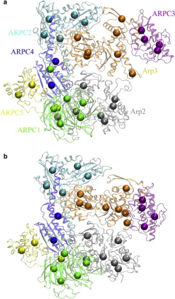
Structures of the Arp2/3 complex at different states and their ENM-ED-CG models. (a) The inactive state and its ENM-ED-CG 34-site model. The number of CG sites in each subunit is: 7 in Arp2 (gray), 7 in Arp3 (orange), 6 in ARPC1 (green), 5 in ARPC2 (cyan), 4 in ARPC3 (purple), 2 in ARPC4 (blue), and 3 in ARPC5 (yellow). (b) The active state and its ENM-ED-CG 34-site model. The number of CG site in each subunit (as the same order and colors as in a) is 7, 8, 5, 5, 4, 2, and 3, respectively. ATP/ADP molecules are not shown because they are not included in ED-CG analyses.

An ENM-ED-CG model was constructed for the inactive and the active Arp2/3 complexes, based on their respective structures. The inactive state was taken from a high resolution crystal structure (PDB accession number: 1K8K) with 1/2 of the Arp2 subunit residues not resolved (43). These missing residues were estimated via homology modeling (51). The active state was obtained from a 3D model of the actin-Arp2/3 branch junction, which was obtained from low resolution fitting of cryo-electron microscopy (cryo-EM) data and remodeling of the high resolution Arp2/3 structure (52).

The Arp2/3 system used in this study has 1923 amino acid residues in the seven subunits plus one ATP and one ADP. As in actin Arp2 and Arp3 bind an adenosine nucleotide. Our system contained ATP-bound Arp3 and ADP-bound Arp2 to reflect the physiological conditions during Arp2/3 activation. To build the ENM, each amino acid residue was taken to have one site (the position of the C_α atom), the ATP molecule four sites (C5, C3^∗, PA, and PG), and the ADP molecule three sites (C5, C3^∗, and PA). After ENM normal modes were calculated, only n = 1923 C_α atoms were used to define ENM-ED-CG models.

The number of CG sites (N) that are needed to represent the whole complex will depend on the properties one wants to address in the CG modeling. In practice, one can predetermine a certain number of ENM modes (n_ED) to be preserved in the resulting CG model, such as the modes that contribute 90% of the total fluctuations. This number of ENM modes will most likely include all the major motions in the complex, such as the protein-protein interactions between subunits. Then, a CG model with the corresponding number of sites (N ≥ (n_ED + 6)/3) is built such that the residual (Eq. 14) is below a certain threshold (notice that the residual will be naturally zero if the CG model goes back to the atomistic model). In the Arp2/3 complex, both the Arp2 and Arp3 subunit share a similar fold as G-actin (43). Therefore seven CG sites are desirable in those two subunits, respectively, to compare with the seven-site model of G-actin. According to the size of the whole system, an ENM-ED-CG model with N = 34 sites was therefore built for the Arp2/3 complex in both states, respectively. The first 96 (=34 × 3 − 6) ENM modes were used, which contribute ∼90% of the total fluctuations.

To reduce the number of boundary atoms to be determined, it is reasonable to assume that a dynamic domain does not cross subunits. That is to say, the C-terminal C_α atom of each subunit is a natural boundary, and there are 34 − 7 = 27 boundary atoms left to be determined. A total of 400 different initial boundary-atom sets were used, and the time cost for ENM-ED-CG of the Arp2/3 complex was only ∼2–3 h on a 2.4 GHz desktop personal computer.

Unlike the cases in the CA dimer and G-actin where many different boundary-atom sets converged to the minimum-residual model, the final 400 sets of the Arp2/3 complex indicate a poor convergence. The model with the lowest residual appears only once in all the 400 final sets, and many other models have very close residuals to the lowest one. The reason may come from the large number of permutations to determine a certain number of boundary atoms from the pool of C_α atoms. The total number of permutations of the Arp2/3 complex optimization problem is $\left(\begin{array}{c}n-7\\ N-7\end{array}\right)\equiv \left(n-7\right)!/\left(\left(N-7\right)!\left(n-N\right)!\right)$. For example, the number of permutations to define a 34-site model is $\left(\begin{array}{c}1916\\ 27\end{array}\right)\approx {10}^{60}$ which is extremely large. There are many local minima with similar residuals, so it will not likely obtain the global minimum by simulated annealing. In the case of poor convergence, it may not be a good strategy to just take the model with the lowest residual because it appears only once randomly in all the final sets and its residual is not significantly lower than others.

Accordingly, the numbers of boundary atoms in each subunit for each of the 400 sets were calculated. Fig. 4 shows the cases of the Arp2 and Arp3 subunits in the inactive Arp2/3 complex. In the 400 initial sets, the numbers of boundary atoms in Arp2 vary from 0 to 13 (Fig. 4 a, dotted line). However, these numbers are much better converged (from 5 to 8) in the 400 final sets after minimization (Fig. 4 a, solid line). It seems that six boundary atoms (seven CG sites) in Arp2 are fairly optimal by taking the average through all the 400 final sets. The results for Arp3 (Fig. 4 b) also suggest the optimal number of CG sites in this subunit is 7. Together with the other six subunits (ARPC1 to ARPC5, data not shown), all the data support the notion that the number of CG sites in each subunit is well converged although the 400 final sets do not converge after minimization. For the 34-site model of the inactive Arp2/3 complex, the optimized numbers of CG sites in the seven subunits are: 7 in Arp2, 7 in Arp3, 6 in ARPC1, 5 in ARPC2, 4 in ARPC3, 2 in ARPC4, and 3 in ARPC5.

Figure 4.

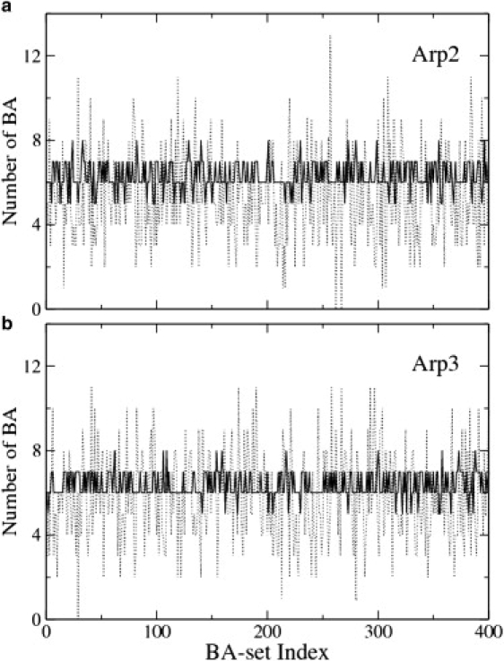
Number of boundary atoms in each subunit of the inactive Arp2/3 complex as a function of the 400 boundary-atom sets. The dotted line shows the numbers in the 400 initial sets, and the solid line shows the corresponding numbers in the final sets after minimization. The latter has a much better convergence. (a) Arp2 subunit. (b) Arp3 subunit.

After determining the numbers of CG sites in all of the subunits, the CG sites in each of them were then optimized, separately. It should be emphasized here that one should still use the ENM modes from the whole complex to compute $\text{t}\text{r}\left[{\left({\mathbf{h}}^{\text{ED}}\right)}_{\text{ij}}^{-1}\right]$ in Eq. 14. to optimize the CG sites in each subunit, separately. It is incorrect to calculate ENM modes of each subunit alone, and then use these modes to define CG sites in the subunit. The ENM modes from the separate subunit do not include any mode related to interactions between the subunits, thus the resulting CG model may not represent protein-protein interactions properly. By this “divide and conquer” strategy, the number of permutations can be largely reduced. Moreover, the convergence was good in each subunit due to its much smaller size than the whole complex. The 34-site model has a residual of 1153.0, which is almost the same as the lowest residual (1151.9) from the final 400 sets. In the latter model, the numbers of CG sites in the seven subunits are: 7 in Arp2, 7 in Arp3, 6 in ARPC1, 4 in ARPC2, 5 in ARPC3, 2 in ARPC4, and 3 in ARPC5. By comparing the two 34-site models (divide and conquer and the lowest-residual model, respectively), they have different numbers of CG sites in the subunits ARPC2 and ARPC3 whereas their residuals are almost the same. This result again indicates that there exist many local minima with very similar residuals for the 34-site models of the complex. The divide and conquer model takes the average boundary-atom distribution among subunits from all the final sets, which should be more robust than a single model with a slightly lower residual.

The 34-site ENM-ED-CG models of the inactive and active Arp2/3 complexes, obtained by the divide and conquer procedure, are shown in Fig. 3. For the 34-site model of the active state, the numbers of CG sites in the seven subunits are: 7 in Arp2, 8 in Arp3, 5 in ARPC1, 5 in ARPC2, 4 in ARPC3, 2 in ARPC4, and 3 in ARPC5. There are many similarities between the 34-site models at the two states. Four subunits (from ARPC2 to ARPC5) have almost the same CG sites between the two states (Fig. 3). ARPC1 has six CG sites at the inactive state, but has only five at the active state. The first four CG sites in ARPC1 are very similar between the two states, whereas the last two CG sites at the inactive state merge into one site at the active state. The major differences between the two states are shown in the Arp2 and Arp3 subunits, which may come from their different essential subspaces. Because ENM is base on a single structure, the ENM modes may be different if there is a conformational change between the two states (Fig. 3). Their RMSIP (Eq. 15) is 0.76 when n_ED = 96. In Arp2, there are seven CG sites for both states (Fig. 5, a and b), and their CG sequence similarity (Eq. 17) is 0.74. Arp3 has seven CG sites too at the inactive state (Fig. 5 c), but eight sites at the active state (Fig. 5 d). Even with different numbers of CG sites, they have a CG sequence similarity of 0.77. The above comparison between the 34-site models for the two states suggests that the Arp2 subunits are most different between the two states, followed by the Arp3 subunits. A proposed model of activation of the inactive complex suggests that a substantial conformational change is required to bring the Arp2 and Arp3 subunits together (44). The Arp2 subunit moves most from its position to overlap with the Arp3 subunit, to initiate the growth of the daughter filaments (44,53). Therefore, it is reasonable that the CG sites in the Arp2 subunit show the greatest difference between the two states. Interestingly, the seven-site model of Arp2 in the active complex (Fig. 5 b) is very similar to the intuitive seven-site model of G-actin (Fig. 2 a). Also six CG sites in Arp3 at the active state (Fig. 5 d, red, blue, cyan, green, orange, and magenta, respectively) look similar to the corresponding CG sites in the intuitive seven-site model of G-actin. These would seem to support the current hypothesis that the Arp2 and Arp3 subunits in the active complex form the first two subunits in the daughter filament (43,52).

Figure 5.

The ENM-ED-CG models of the Arp2 and Arp3 subunits from the 34-site models of the Arp2/3 complex (Fig. 3). (a) The seven-site model of Arp2 in the inactive Arp2/3 complex (Fig. 3a, gray). (b) The seven-site model of Arp2 in the active Arp2/3 complex (Fig. 3b, gray). (c) The seven-site model of Arp3 in the inactive Arp2/3 complex (Fig. 3a, orange). (d) The eight-site model of Arp3 in the active Arp2/3 complex (Fig. 3b, orange).

Conclusions

ENMs of biomolecules are widely used in CG modeling to study functional dynamics of proteins or supramolecular complexes of proteins (5–13), in which an amino acid is often reduced to one CG site (for example, at the position of the C_α atom). A new ED-CG scheme has been implemented here using ENM to define a CG model of a biomolecule with a much lower resolution than one site per residue, which significantly extends our method developed previously (26). Coarse-grained normal modes are computed by ENM, and these low-frequency modes are used to construct a functionally important essential dynamics subspace. Then the CG sites are variationally determined to preserve dynamic domains and reflect essential dynamics described by the low-frequency normal modes.

The ENM-ED-CG method has also been applied here to several biologically important systems. Two proteins, the HIV-1 CA protein dimer (CA dimer) and ATP-bound G-actin, were used for comparison with our previous results obtained with ED-CG based on PCA from an MD trajectory. The symmetric ENM-ED-CG four-, six-, and eight-site models of the CA dimer are almost the same as those obtained with MD + PCA. The ED-CG seven-site models between ENM and PCA are also quite similar according to their quantitative CG sequence similarity (Eq. 17).

In the case of CG models of the Arp2/3 complex, it is, to our knowledge, the first time ED-CG has been carried out on such a large multi-protein assembly (e.g., a system significantly larger than the HIV-1 CA dimer and G-actin). The ENM-ED-CG analysis was finished in a fairly short time (2–3 h) on a regular desktop computer, which indicates that the method may readily handle even larger biomolecular complexes. However, the complexity to define a 34-site model of the Arp2/3 complex is significant and the convergence of the algorithm suffers due to the large number of possible permutations. In this case, the model with the lowest residual in all the final sets is most likely not the global minimum. It may not be a good representative of the ENM-ED-CG model of the Arp2/3 complex because it is just a random set that appears only once and its residual is not significantly lower than many other models. Therefore, a divide and conquer procedure should be used to obtain a more robust ENM-ED-CG model of the complex, which can be divided into two steps. The first step is to take the average number of CG sites in each subunit from the 400 final sets, which converges quite well after minimization (Fig. 4). After an optimal number of CG sites in each subunit are determined, the second step is to variationally optimize the positions of CG sites in each subunit, separately. Through this divide and conquer strategy, the computational complexity (the number of possible permutations) is substantially reduced and the convergence of the algorithm in each subunit is far superior. The CG model obtained by this two-step strategy should be more robust than the model with the lowest residual because it is an average of all the final sets that can remove the random noise from any single set. In the mean time, the residual of the divide and conquer model is usually as low as the lowest residual. The resulting ENM-ED-CG 34-site models of the inactive and active Arp2/3 complex show good agreement with the experimental structural data and current activation model.

For a system like the Arp2/3 complex, or an even larger biomolecule, it would be computationally expensive to perform a very long time atomistic MD simulation so as to achieve a converged PCA. Moreover, because the lowest-frequency PCA modes (and those most relevant to define ED-CG models based on PCA) in a system take the longest to converge (54), the required amount of MD simulation time for developing CG models of large complexes may well be prohibitive at this time. A main advantage of the ENM-ED-CG method, therefore, is that one can readily build a CG model based on ENM modes from a single structure instead of relying on PCA modes obtained from a MD trajectory, because no MD simulation is needed in the former.

ENM modes are calculated from a single structure. If a biomolecular system has distinct conformational states, the ENM modes between them will be more or less different, which may lead to different ENM-ED-CG models. The construction of a proper ED-CG model that captures the dynamics at several conformational states remains to be addressed, to study conformational transitions between multiple states by CG modeling.

Before using the ENM-ED-CG method, one should also pay close attention to the quality of ENM modes. Sometimes an ENM may reproduce a so-called “tip effect” (10). A “tip”, which is usually a region protruding out of the main body of the biomolecule, may have unrealistic large amplitude fluctuations probably due to its few and unbalanced elastic interactions with the other regions in ENM. This artifact may affect the quality of the ENM modes even with low frequencies, which will lead to unreasonable ENM-ED-CG models because protein dynamics described by these ENM modes are unrealistic. The tip effect was not observed in all the three systems in this article by using a regular ENM. If it happens, a modified ENM with a more complicated elastic potential (10) can be used to eliminate this artifact systematically.

A potential use of the ENM-ED-CG method is to define CG models directly from low-resolution structural data obtained by cryo-EM. The technique of cryo-EM can provide low-resolution structures of many large biomolecular assemblies (55,56), which are difficult to study by x-ray crystallography or NMR. A number of such studies indicate that these low-resolution structures are sufficient to provide at least low-frequency dynamics of biomolecular systems because they mainly depend on the shape of the biomolecule rather than on its atomic details (8,57). Therefore the ENM-ED-CG method can be applied to these low-resolution structures with less accuracy than the atomistic model. In particular, a vector quantization approach is used to discretize the cryo-EM density map into a set of landmark points (58,59), and an ENM with these points is then built to represent the cryo-EM structure (18–20). After the normal modes are calculated by this model, the ENM-ED-CG method can be applied to define CG sites for these low-resolution structures. This avenue of research will be explored in the future both in a general sense and for particular important biomolecular systems.

References

- 1.Voth G.A. CRC Press-Taylor & Francis Group; Boca Raton, FL: 2009. Coarse-Graining of Condensed Phase and Biomolecular Systems. [Google Scholar]
- 2.Tozzini V. Coarse-grained models of proteins. Curr. Opin. Struct. Biol. 2005;15:144–150. doi: 10.1016/j.sbi.2005.02.005. [DOI] [PubMed] [Google Scholar]
- 3.Ayton G.S., Noid W.G., Voth G.A. Multiscale modeling of biomolecular systems: in serial and in parallel. Curr. Opin. Struct. Biol. 2007;17:192–198. doi: 10.1016/j.sbi.2007.03.004. [DOI] [PubMed] [Google Scholar]
- 4.Murtola T., Bunker A., Vattulainen I., Deserno M., Karttunen M. Multiscale modeling of emergent materials: biological and soft matter. Phys. Chem. Chem. Phys. 2009;11:1869–1892. doi: 10.1039/b818051b. [DOI] [PubMed] [Google Scholar]
- 5.Tirion M.M. Large amplitude elastic motions in proteins from a single-parameter atomic analysis. Phys. Rev. Lett. 1996;77:1905–1908. doi: 10.1103/PhysRevLett.77.1905. [DOI] [PubMed] [Google Scholar]
- 6.Atilgan A.R., Durell S.R., Jernigan R.L., Demirel M.C., Keskin O. Anisotropy of fluctuation dynamics of proteins with an elastic network model. Biophys. J. 2001;80:505–515. doi: 10.1016/S0006-3495(01)76033-X. [DOI] [PMC free article] [PubMed] [Google Scholar]
- 7.Bahar I., Rader A.J. Coarse-grained normal mode analysis in structural biology. Curr. Opin. Struct. Biol. 2005;15:586–592. doi: 10.1016/j.sbi.2005.08.007. [DOI] [PMC free article] [PubMed] [Google Scholar]
- 8.Lu M.Y., Ma J.P. The role of shape in determining molecular motions. Biophys. J. 2005;89:2395–2401. doi: 10.1529/biophysj.105.065904. [DOI] [PMC free article] [PubMed] [Google Scholar]
- 9.Ma J.P. Usefulness and limitations of normal mode analysis in modeling dynamics of biomolecular complexes. Structure. 2005;13:373–380. doi: 10.1016/j.str.2005.02.002. [DOI] [PubMed] [Google Scholar]
- 10.Lu M.Y., Poon B., Ma J.P. A new method for coarse-grained elastic normal-mode analysis. J. Chem. Theory Comput. 2006;2:464–471. doi: 10.1021/ct050307u. [DOI] [PMC free article] [PubMed] [Google Scholar]
- 11.Yang L., Song G., Jernigan R.L. How well can we understand large-scale protein motions using normal modes of elastic network models? Biophys. J. 2007;93:920–929. doi: 10.1529/biophysj.106.095927. [DOI] [PMC free article] [PubMed] [Google Scholar]
- 12.Moritsugu K., Smith J.C. Coarse-grained biomolecular simulation with REACH: Realistic extension algorithm via covariance Hessian. Biophys. J. 2007;93:3460–3469. doi: 10.1529/biophysj.107.111898. [DOI] [PMC free article] [PubMed] [Google Scholar]
- 13.Lyman E., Pfaendtner J., Voth G.A. Systematic multiscale parameterization of heterogeneous elastic network models of proteins. Biophys. J. 2008;95:4183–4192. doi: 10.1529/biophysj.108.139733. [DOI] [PMC free article] [PubMed] [Google Scholar]
- 14.Keskin O., Bahar I., Flatow D., Covell D.G., Jernigan R.L. Molecular mechanisms of chaperonin GroEL-GroES function. Biochemistry. 2002;41:491–501. doi: 10.1021/bi011393x. [DOI] [PubMed] [Google Scholar]
- 15.Tama F., Valle M., Frank J., Brooks C.L. Dynamic reorganization of the functionally active ribosome explored by normal mode analysis and cryo-electron microscopy. Proc. Natl. Acad. Sci. USA. 2003;100:9319–9323. doi: 10.1073/pnas.1632476100. [DOI] [PMC free article] [PubMed] [Google Scholar]
- 16.Wang Y.M., Rader A.J., Bahar I., Jernigan R.L. Global ribosome motions revealed with elastic network model. J. Struct. Biol. 2004;147:302–314. doi: 10.1016/j.jsb.2004.01.005. [DOI] [PubMed] [Google Scholar]
- 17.Kurkcuoglu O., Doruker P., Sen T.Z., Kloczkowski A., Jernigan R.L. The ribosome structure controls and directs mRNA entry, translocation and exit dynamics. Phys. Biol. 2008;5:46005. doi: 10.1088/1478-3975/5/4/046005. [DOI] [PMC free article] [PubMed] [Google Scholar]
- 18.Ming D., Kong Y., Lambert M.A., Huang Z., Ma J. How to describe protein motion without amino acid sequence and atomic coordinates. Proc. Natl. Acad. Sci. USA. 2002;99:8620–8625. doi: 10.1073/pnas.082148899. [DOI] [PMC free article] [PubMed] [Google Scholar]
- 19.Ming D., Kong Y., Wakil S.J., Brink J., Ma J. Domain movements in human fatty acid synthase by quantized elastic deformation model. Proc. Natl. Acad. Sci. USA. 2002;99:7895–7899. doi: 10.1073/pnas.112222299. [DOI] [PMC free article] [PubMed] [Google Scholar]
- 20.Tama F., Wriggers W., Brooks C.L. Exploring global distortions of biological macromolecules and assemblies from low-resolution structural information and elastic network theory. J. Mol. Biol. 2002;321:297–305. doi: 10.1016/s0022-2836(02)00627-7. [DOI] [PubMed] [Google Scholar]
- 21.Chu J.W., Voth G.A. Allostery of actin filaments: molecular dynamics simulations and coarse-grained analysis. Proc. Natl. Acad. Sci. USA. 2005;102:13111–13116. doi: 10.1073/pnas.0503732102. [DOI] [PMC free article] [PubMed] [Google Scholar]
- 22.Chu J.W., Voth G.A. Coarse-grained modeling of the actin filament derived from atomistic-scale simulations. Biophys. J. 2006;90:1572–1582. doi: 10.1529/biophysj.105.073924. [DOI] [PMC free article] [PubMed] [Google Scholar]
- 23.Arkhipov A., Freddolino P.L., Imada K., Namba K., Schulten K. Coarse-grained molecular dynamics simulations of a rotating bacterial flagellum. Biophys. J. 2006;91:4589–4597. doi: 10.1529/biophysj.106.093443. [DOI] [PMC free article] [PubMed] [Google Scholar]
- 24.Arkhipov A., Freddolino P.L., Schulten K. Stability and dynamics of virus capsids described by coarse-grained modeling. Structure. 2006;14:1767–1777. doi: 10.1016/j.str.2006.10.003. [DOI] [PubMed] [Google Scholar]
- 25.Arkhipov A., Yin Y., Schulten K. Four-scale description of membrane sculpting by BAR domains. Biophys. J. 2008;95:2806–2821. doi: 10.1529/biophysj.108.132563. [DOI] [PMC free article] [PubMed] [Google Scholar]
- 26.Zhang Z., Lu L., Noid W.G., Krishna V., Pfaendtner J. A systematic methodology for defining coarse-grained sites in large biomolecules. Biophys. J. 2008;95:5073–5083. doi: 10.1529/biophysj.108.139626. [DOI] [PMC free article] [PubMed] [Google Scholar]
- 27.Amadei A., Linnsen A.B.M., Berendsen H.J.C. Essential dynamics of proteins. Proteins. 1993;17:412–425. doi: 10.1002/prot.340170408. [DOI] [PubMed] [Google Scholar]
- 28.Kitao A., Go N. Investigating protein dynamics in collective coordinate space. Curr. Opin. Struct. Biol. 1999;9:164–169. doi: 10.1016/S0959-440X(99)80023-2. [DOI] [PubMed] [Google Scholar]
- 29.Berendsen H.J.C., Hayward S. Collective protein dynamics in relation to function. Curr. Opin. Struct. Biol. 2000;10:165–169. doi: 10.1016/s0959-440x(00)00061-0. [DOI] [PubMed] [Google Scholar]
- 30.Kuriyan J., Petsko G.A., Levy R.M., Karplus M. Effect of anisotropy and anharmonicity on protein crystallographic refinement—an evaluation by molecular dynamics. J. Mol. Biol. 1986;190:227–254. doi: 10.1016/0022-2836(86)90295-0. [DOI] [PubMed] [Google Scholar]
- 31.Ichiye T., Karplus M. Anisotropy and anharmonicity of atomic fluctuations in proteins - analysis of a molecular dynamics simulation. Proteins. 1987;2:236–259. doi: 10.1002/prot.340020308. [DOI] [PubMed] [Google Scholar]
- 32.Doruker P., Atilgan A.R., Bahar I. Dynamics of proteins predicted by molecular dynamics simulations and analytical approaches: application to alpha-amylase inhibitor. Proteins. 2000;40:512–524. [PubMed] [Google Scholar]
- 33.Flory P.J., Gordon M., McCrum N.G. Statistical thermodynamics of random networks [and discussion] Proc. R. Soc. Lond. A Math. Phys. Sci. 1976;351:351–380. [Google Scholar]
- 34.Kirkpatrick S., Gelatt J.C.D., Vecchi M.P. Optimization by simulated annealing. Science. 1983;220:671–680. doi: 10.1126/science.220.4598.671. [DOI] [PubMed] [Google Scholar]
- 35.Li S., Hill C.P., Sundquist W.I., Finch J.T. Image reconstructions of helical assemblies of the HIV-1 CA protein. Nature. 2000;407:409–413. doi: 10.1038/35030177. [DOI] [PubMed] [Google Scholar]
- 36.Amadei A., Ceruso M.A., Di Nola A. On the convergence of the conformational coordinates basis set obtained by the essential dynamics analysis of proteins' molecular dynamics simulations. Proteins. 1999;36:419–424. [PubMed] [Google Scholar]
- 37.Graceffa P., Dominguez R. Crystal structure of monomeric actin in the ATP state. Structural basis of nucleotide-dependent actin dynamics. J. Biol. Chem. 2003;278:34172–34180. doi: 10.1074/jbc.M303689200. [DOI] [PubMed] [Google Scholar]
- 38.Kabsch W., Mannherz H.G., Suck D., Pai E.F., Holmes K.C. Atomic structure of the actin: DNase I complex. Nature. 1990;347:37–44. doi: 10.1038/347037a0. [DOI] [PubMed] [Google Scholar]
- 39.Khaitlina S.Y., Moraczewska J., Strzeleckagolaszewska H. The actin/actin interactions involving the N-terminus of the DNase-I-binding loop are crucial for stabilization of the actin filament. Eur. J. Biochem. 1993;218:911–920. doi: 10.1111/j.1432-1033.1993.tb18447.x. [DOI] [PubMed] [Google Scholar]
- 40.Pfaendtner J., Branduardi D., Parrinello M., Pollard T.D., Voth G.A. Nucleotide-dependent conformational states of actin. Proc. Natl. Acad. Sci. USA. 2009;106:12723–12728. doi: 10.1073/pnas.0902092106. [DOI] [PMC free article] [PubMed] [Google Scholar]
- 41.Pollard T.D., Beltzner C.C. Structure and function of the Arp2/3 complex. Curr. Opin. Struct. Biol. 2002;12:768–774. doi: 10.1016/s0959-440x(02)00396-2. [DOI] [PubMed] [Google Scholar]
- 42.May R.C. The Arp2/3 complex: a central regulator of the actin cytoskeleton. Cell. Mol. Life Sci. 2001;58:1607–1626. doi: 10.1007/PL00000800. (CMLS) [DOI] [PMC free article] [PubMed] [Google Scholar]
- 43.Robinson R.C., Turbedsky K., Kaiser D.A., Marchand J.B., Higgs H.N. Crystal structure of Arp2/3 complex. Science. 2001;294:1679–1684. doi: 10.1126/science.1066333. [DOI] [PubMed] [Google Scholar]
- 44.Pollard T.D. Regulation of actin filament assembly by Arp2/3 complex and formins. Annu. Rev. Biophys. Biomol. Struct. 2007;36:451–477. doi: 10.1146/annurev.biophys.35.040405.101936. [DOI] [PubMed] [Google Scholar]
- 45.Dayel M.J., Holleran E.A., Mullins R.D. Arp2/3 complex requires hydrolyzable ATP for nucleation of new actin filaments. Proc. Natl. Acad. Sci. USA. 2001;98:14871–14876. doi: 10.1073/pnas.261419298. [DOI] [PMC free article] [PubMed] [Google Scholar]
- 46.Le Clainche C., Pantaloni D., Carlier M.F. ATP hydrolysis on actin-related protein 2/3 complex causes debranching of dendritic actin arrays. Proc. Natl. Acad. Sci. USA. 2003;100:6337–6342. doi: 10.1073/pnas.1130513100. [DOI] [PMC free article] [PubMed] [Google Scholar]
- 47.Goley E.D., Rodenbusch S.E., Martin A.C., Welch M.D. Critical conformational changes in the Arp2/3 complex are induced by nucleotide and nucleation promoting factor. Mol. Cell. 2004;16:269–279. doi: 10.1016/j.molcel.2004.09.018. [DOI] [PubMed] [Google Scholar]
- 48.Egile C., Rouiller I., Xu X.P., Volkmann N., Li R. Mechanism of filament nucleation and branch stability revealed by the structure of the Arp2/3 complex at actin branch junctions. PLoS Biol. 2005;3:1902–1909. doi: 10.1371/journal.pbio.0030383. [DOI] [PMC free article] [PubMed] [Google Scholar]
- 49.Martin A.C., Xu X.P., Rouiller I., Kaksonen M., Sun Y.D. Effects of Arp2 and Arp3 nucleotide-binding pocket mutations on Arp2/3 complex function. J. Cell Biol. 2005;168:315–328. doi: 10.1083/jcb.200408177. [DOI] [PMC free article] [PubMed] [Google Scholar]
- 50.Kiselar J.G., Mahaffy R., Pollard T.D., Almo S.C. Visualizing Arp2/3 complex activation mediated by binding of ATP and WASp using structural mass spectrometry. Proc. Natl. Acad. Sci. USA. 2007;104:1552–1557. doi: 10.1073/pnas.0605380104. [DOI] [PMC free article] [PubMed] [Google Scholar]
- 51.Pfaendtner J., Voth G.A. Molecular dynamics simulation and coarse-grained analysis of the Arp2/3 complex. Biophys. J. 2008;95:5324–5333. doi: 10.1529/biophysj.108.143313. [DOI] [PMC free article] [PubMed] [Google Scholar]
- 52.Rouiller I., Xu X.P., Amann K.J., Egile C., Nickell S. The structural basis of actin filament branching by the Arp2/3 complex. J. Cell Biol. 2008;180:887–895. doi: 10.1083/jcb.200709092. [DOI] [PMC free article] [PubMed] [Google Scholar]
- 53.Gournier H., Goley E.D., Niederstrasser H., Trinh T., Welch M.D. Reconstitution of human Arp2/3 complex reveals critical roles of individual subunits in complex structure and activity. Mol. Cell. 2001;8:1041–1052. doi: 10.1016/s1097-2765(01)00393-8. [DOI] [PubMed] [Google Scholar]
- 54.Hess B. Similarities between principal components of protein dynamics and random diffusion. Phys. Rev. E. 2000;62:8438–8448. doi: 10.1103/physreve.62.8438. [DOI] [PubMed] [Google Scholar]
- 55.Saibil H.R. Conformational changes studied by cryo-electron microscopy. Nat. Struct. Biol. 2000;7:711–714. doi: 10.1038/78923. [DOI] [PubMed] [Google Scholar]
- 56.Joachim F. Oxford University Press; New York: 2006. Three-Dimensional Electron Microscopy of Macromolecular Assemblies. [Google Scholar]
- 57.Tama F., Brooks C.L. Symmetry, form, and shape: guiding principles for robustness in macromolecular machines. Annu. Rev. Biophys. Biomol. Struct. 2006;35:115–133. doi: 10.1146/annurev.biophys.35.040405.102010. [DOI] [PubMed] [Google Scholar]
- 58.Wriggers W., Milligan R.A., Schulten K., McCammon J.A. Self-organizing neural networks bridge the biomolecular resolution gap. J. Mol. Biol. 1998;284:1247–1254. doi: 10.1006/jmbi.1998.2232. [DOI] [PubMed] [Google Scholar]
- 59.Wriggers W., Chacón P., Kovacs J., Tama F., Birmanns S. Topology representing neural networks reconcile biomolecular shape, structure, and dynamics. Neurocomputing. 2004;56:165–179. [Google Scholar]
- 60.Humphrey W., Dalke A., Schulten K. VMD: visual molecular dynamics. J. Mol. Graph. 1996;14:33–38. doi: 10.1016/0263-7855(96)00018-5. [DOI] [PubMed] [Google Scholar]