Abstract
In study of early brain development, tissue segmentation of neonatal brain MR images remains challenging because of the insufficient image quality due to the properties of developing tissues.. Among various brain tissue segmentation algorithms, atlas-based brain image segmentation can potentially achieve good segmentation results on neonatal brain images. However, their performances rely on both the quality of the atlas and the spatial correspondence between the atlas and the to-be-segmented image. Moreover, it is difficult to build a population atlas for neonates due to the requirement of a large set of tissue-segmented neonatal brain images. To combat these obstacles, we present a longitudinal neonatal brain image segmentation framework by taking advantage of the longitudinal data acquired at late time-point to build a subject-specific tissue probabilistic atlas. Specifically, tissue segmentation of the neonatal brain is formulated as two iterative steps of bias correction and probabilistic-atlas-based tissue segmentation, along with the longitudinal atlas reconstructed by the late time image of the same subject. The proposed method has been evaluated qualitatively through visual inspection and quantitatively by comparing with manual delineations and two population-atlas-based segmentation methods. Experimental results show that the utilization of a subject-specific probabilistic atlas can substantially improve tissue segmentation of neonatal brain images.
Keywords: Neonate, Tissue segmentation, Probabilistic atlas, Subject-specific atlas
Introduction
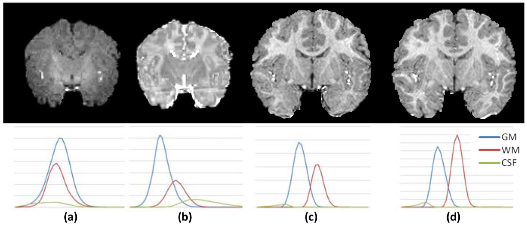
Longitudinal MRI study in neonates has the potential to reveal the early brain development patterns (Dubois et al., 2008; Gerig et al., 2006; Knickmeyer et al., 2008). To perform quantitative analysis of longitudinal MR images in global and local brain regions, such as tissue volume measurement, inter-tissue boundary detection, and cortical surface and thickness evaluation, an essential procedure is to segment brain images into anatomically meaningful tissues such as gray matter (GM), white matter (WM), and cerebrospinal fluid (CSF). The accuracy of tissue segmentation is crucial for subsequent quantitative analysis. However, despite the success of brain tissue segmentation algorithms developed for adult and pediatric brain images (Pham et al., 2000), it remains challenging to segment neonatal brain images (Mewes et al., 2006; Prastawa et al., 2005; Xue et al., 2007) because of poor spatial resolution, low tissue contrast, and high within-tissue intensity variability. As shown in Fig. 1(a–b), in the neonatal MR T1 and T2 images, tissue intensity distributions of GM, WM, and CSF largely overlap, especially in the T1 image (Fig. 1a). Hindered by these difficulties, intensity-based segmentation algorithms, built upon an assumption that image intensities of a same brain tissue have a compact distribution, generally fail to segment neonatal brain images. Sometimes, it is difficult even for experts to visually distinguish between different neonatal brain tissues (Nishida et al., 2006; Song et al., 2007). However, it is worth noting that the quality of MRI brain images of one-year-old and two-year-old is much better as shown in Fig.1(c–d). This suggests that the image acquired at the late time-point is relatively easier to segment than the image acquired at neonatal stage. Thus, the segmentation result of the late time image can be potentially used to help the segmentation of neonatal brain image.
Fig. 1.
Representative longitudinal MR images and corresponding tissue intensity distributions of a subject. (a) T1 image at neonate; (b) T2 image at neonate; (c) T1 image at one-year-old; and (d) T1 image at two-year-old.
In the literature, the knowledge-based segmentation algorithms have been developed for neonatal brain image segmentation (Bazin and Pham, 2007; Nishida et al., 2006; Pham and Prince, 1999; Prastawa et al., 2005; Song et al., 2007; Warfield et al., 2000; Weisenfeld and Warfield, 2009; Xue et al., 2007). These algorithms perform brain tissue segmentation under the guidance of an atlas that encodes prior knowledge of anatomical structures’ spatial locations, shapes, as well as their spatial relationships. A typical atlas generally comprises an intensity image, which can be used as an intensity model for atlas-to-subject registration, and also the probabilistic maps of GM, WM, and CSF, which can be used as prior tissue probability maps for guiding segmentation. The atlas can be generated by manually or automatically segmenting an individual image, or integrating information from multiple segmented images of different individual subjects.
For optimizing the performance of atlas-based segmentation on neonatal brain images, various atlases have been constructed. Due to high inter-subject anatomical variability, it is difficult for the atlas of an individual brain image to achieve a good segmentation performance, when applied to images with different anatomical structures. Researchers then turned to use the atlas built on multiple images. Prastawa et al. generated an atlas by averaging three semi-automatic segmented neonatal brain images, registered with affine transformation (Prastawa et al., 2005). Song et al. built an unbiased atlas from 9 of 10 neonates in a leave-one-out manner with diffeomorphic flow-based registration (Song et al., 2007). To minimize the age-related anatomical difference between images used for generating the atlas and the to-be-segmented image, Warfield et al. employed an age-specific atlas and proposed an iterated tissue segmentation and atlas alignment strategy to improve the neonatal tissue segmentation (Warfield et al., 2000). Xue et al. constructed multiple age-specific atlases and performed an expectation-maximization (EM) algorithm for tissue segmentation, in conjunction with Markov random field (MRF) to remove the mislabeled partial volume voxels in an iterative manner (Xue et al., 2007). Likewise, Aljabar et al. demonstrated that an atlas built from images similar to the to-be–segmented image can achieve better segmentation accuracy than atlases built from images randomly selected (Aljabar et al., 2009). These studies indicate that, for achieving good segmentation performance, it is necessary to have an atlas with similar anatomical structures with the to-be-segmented image, which we consider as a good atlas for guiding segmentation. On the other hand, the atlas built on multiple images can appear from blurry to sharp, depending on different setting of registration regularization in the atlas construction process, i.e., from strong to weak regularization (Thomas Yeo et al., 2008). The optimal atlas sharpness degree needs to be explored in order to maximize the guiding power of atlas and achieve the best segmentation performance.
In atlas-based image segmentation algorithms, the segmentation performance is also affected by the registration procedure of registering the atlas to the to-be-segmented image. Different registration procedures typically yield different segmentation results even using the same atlas and the same subject image (Rohlfing et al., 2003). Therefore, an effective registration strategy is needed to estimate the spatial correspondence between the atlas and the to-be-segmented image for the accurate incorporation of the prior knowledge embedded in the atlas.
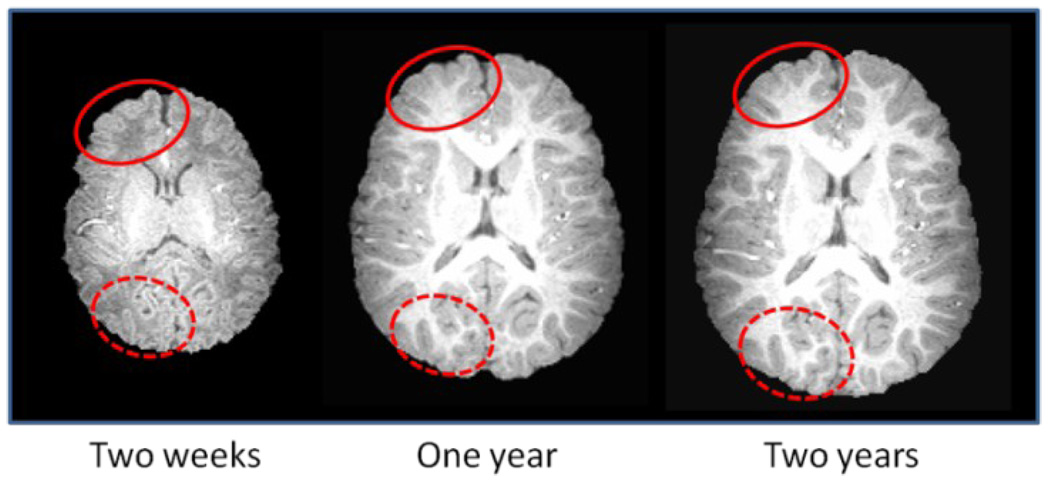
In longitudinal studies, a subject is scanned at multiple time-points. Thus, the images of a same subject acquired at different time-points have similar anatomical structures since major cortical gyrification develops during gestation of third trimester, and cortical convolution patterns remain similar after normal birth (Armstrong et al., 1995). The similarity of anatomical structures of the same subject at different development stages is observable in MRI images. As shown in Fig. 2, white matter pattern within the solid (and dashed) circles is very similar across images acquired at two weeks, one year, and two years old of the same subject. Since the segmentation of late time brain image such as two-year-old (or even one-year-old) can be achieved with high accuracy using existing segmentation methods like fuzzy clustering (Fig. 4), we propose to use a late-time-point image in conjunction with its segmentation result as a subject-specific tissue probabilistic atlas to guide tissue segmentation of the neonatal image. Compared with the atlases built from images of different individuals, the subject-specific atlas has smaller anatomical variability, thus has a potential to better guide tissue segmentation of the neonatal image. In particular, the subject-specific atlas can be used within a joint registration-segmentation framework to perform atlas alignment and image segmentation of the neonatal image.
Fig. 2.
Demonstration of the similarity of the cortical convolution pattern in the images of a same subject acquired at two weeks, one year old, and two years old. Red circles are provided for easy comparison of local cortical folds across different time points.
Fig. 4.
Tissue segmentation results for a two-year-old brain image. (a) Original T1 image; (b) Tissue segmentation result; and probabilistic maps of (c) GM, (d) WM, and (e) CSF.
This paper is organized as follows. Details of the proposed segmentation framework are presented in the method section. Then, an experiment section presents the segmentation results produced by the proposed method, and the comparisons with manual delineations and two population-atlas-based segmentation methods. Finally, the paper is concluded with a discussion.
Method
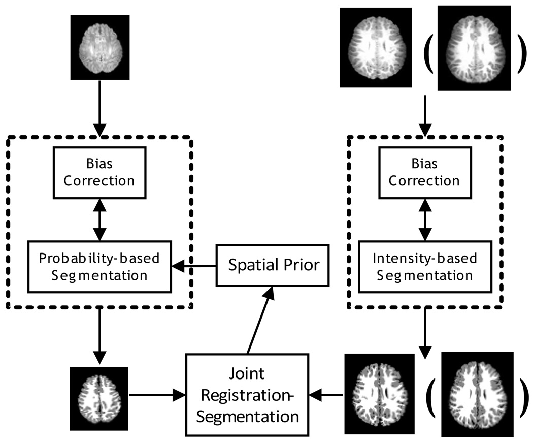
In this paper, we propose to use a subject-specific atlas constructed from the image acquired at late time-point (e.g., one-year-old or two-year-old) of the same subject for guiding neonatal image segmentation. As summarized in Fig. 3, our algorithm consists of two components: (1) Fuzzy segmentation of late time images and construction of tissue probabilistic atlas, as shown in the right panel of Fig. 3; (2) Joint registration-segmentation step for atlas alignment and atlas-based tissue segmentation of the neonatal image, as shown in the left panel of Fig. 3. Specifically, in the joint registration and segmentation step, we iteratively performed atlas registration, bias field correction, and atlas-based tissue segmentation. It is worth noting that the tissue segmentation results of different time-points, for example, the one-year-old and two-year-old images, can both be used to guide the neonatal image segmentation. Their performances are compared and provided in the experiment section, to evaluate the possible variance of neonatal segmentation results with different time-points.
Fig. 3.
The proposed tissue segmentation framework. The images in the top row are the original MR images acquired at approximately two weeks, one year old (or two years old). The images in the bottom row are the corresponding segmentation results.
In MR image segmentation, T1 image is usually chosen for its higher spatial resolution and tissue contrast. However, for neonates, T2 image has better tissue contrast than T1 image as illustrated in Fig. 1(a–b). For this reason, most neonatal segmentation algorithms either combine T1 and T2 images (Prastawa et al., 2005; Weisenfeld and Warfield, 2009), or use T2 images solely (Song et al., 2007; Xue et al., 2007) for tissue segmentation. In this study, we choose to use T2 images for neonatal brain segmentation, and T1 images for one-year-old and two-year-old brain segmentation.
In the following subsections, we describe our proposed segmentation framework by first introducing the preprocessing steps such as skull-stripping and cerebellum removal, and then detailing the subject-specific atlas construction and the joint registration and segmentation approach.
2.1 Preprocessing step
Preprocessing is a standard procedure in general brain image segmentation, aiming to reduce image noise and remove skull, eyes, and cerebellum before segmentation (Kwon et al., 2003). Many algorithms have been developed to remove the non-brain tissues such as skull and extra-cranial tissues, including Brain Surface Extractor (BSE) (Shattuck and Leahy, 2001) and Brain Extraction Tool (BET) (Smith, 2002). We employ both algorithms (with adjusted parameters) for skull stripping of all time-point images, followed by manual editing to ensure accurate skull removal especially for neonatal images, in which intensity inhomogeneity makes it difficult to obtain satisfactory skull-stripping results with these automatic algorithms. We then manually removed the cerebellum and brain stem in all images, to focus on segmentation of only cerebrum (although we still call it as brain segmentation, instead of cerebrum segmentation in this paper). Examples of skull-stripped and cerebellum-removed brain images can be observed in Fig 1.
2.2 Construction of subject-specific atlas from image acquired at late time-point
To construct a subject-specific atlas for neonatal segmentation, the late time-point image of the same subject is first segmented by a fuzzy segmentation algorithm (Pham and Prince, 1999), to generate tissue probabilistic maps of GM, WM, and CSF.
The fuzzy segmentation, also referred to as fuzzy clustering, is derived from the K-means algorithm (Pham et al., 2000), which segments an image by iteratively computing a mean intensity for each class and classifying voxels into the class with the closest intensity centroid. Due to the partial volume effect, each voxel could be a combination of GM, WM and CSF. The fuzzy c-means (FCM) algorithm (Bezdek and Ehrlich, 1984) handles this problem by using memberships to model each voxel’s fuzziness. The membership measures the fuzziness of each voxel belonging to different classes. In particular, the standard FCM minimizes the following objective function to find the fuzzy membership functions µ and the centroids c in a given image I:
| (1) |
where for each voxel j in an image domain, Ij is the observed image intensity, ck is the centroid of class k, μj,k is the membership value of class k in the voxel j, and q is the weighting exponent on each fuzzy membership to determine the amount of fuzziness of the resulting classification. The parameter q is generally set as 2 in many applications (Pham et al., 1997).
However, the standard FCM cannot deal with the possible intensity inhomogeneity in MR images, which can affect the intensity distribution of brain tissues and the performance of fuzzy clustering. This problem was effectively solved by the adaptive fuzzy c-means (AFCM) algorithm (Pham and Prince, 1999), which simultaneously performs fuzzy clustering and intensity inhomogeneity estimation. Briefly, the following objective function needs to be minimized:
| (2) |
where gi is the bias field in voxel j, which models the intensity inhomogeneity. Dr and Ds are the finite difference operators along the r -th and s -th dimension of the image, with r, s, ∈ {1,2,3} in this study. The last two terms of equation (2) are the first and second-order regularization terms for restricting the bias field to be smooth and vary slowly. To solve this equation, the centroids are first computed by estimating the image histogram, and used to get membership of each voxel for each class. The bias field is estimated by computing the space-varying difference.
Here, we adopt the AFCM method to perform a soft segmentation of the late time-point image, and get the probabilistic maps of three tissues, namely WM, GM, and CSF probabilistic maps. The centroid ck is initialized as equal interval from minimum to maximum of image intensity for CSF, GM, and WM, and gj is set as 1 uniformly in the whole image initially. By iteratively updating the centroids and the bias field, the segmentation converges when the maximal change in the membership functions over all voxels between two iterations is less than a given threshold.
The typical tissue segmentation result of a two-year-old image produced by this iterative procedure is shown in Fig. 4. It is worth noting that the above steps also generate three tissue probabilistic maps for GM, WM, and CSF, respectively, which can be used as subject-specific tissue probabilistic atlas to guide the segmentation of neonatal brain image as detailed below.
Yeo et al. indicated that the sharpness (or smoothness) of atlas has an influence on image segmentation (Yeo et al., 2008). For example, the segmentation results with strong atlas will more rely on the atlas (instead of the intensity information of the image itself), and will produce results similar to the atlas; while weak atlas has insufficient prior information and thus generally results in a loss of details in tissue segmentation results. In this paper, we follow to use the term sharpness to describe the similar influence on segmentation with individual atlas, when adjusting the balance between the individual atlas (appearing sharp) and a uniformly distributed prior (i.e., no preference on any tissue, appearing blurry). To explore the effects of segmentation accuracy with respect to the sharpness of the individual atlas, we introduce a parameter t to control the balance as follows:
| (3) |
where pj,k is the probability of tissue class k in a given voxel j, K is the total number of brain tissues (K = 3 in this study), is a new adjusted tissue probability. When t is 1, the original sharp individual atlas is used. When t is 0, all tissue probabilities are equally distributed and this uniform global prior is used. By optimizing the parameter t, we can adjust the percentage of longitudinal information used to guide tissue segmentation, and eventually achieve better segmentation performance. This exploration of t values will be provided in the experiment section.
2.3 Joint registration-segmentation of neonatal image
Atlas-based segmentation algorithms generally comprise two steps: 1) a registration step for bringing the atlas onto the coordinate space of the to-be-segmented image, and 2) a segmentation step for atlas-based tissue segmentation. Such a two-step process can be done sequentially (Cocosco et al., 2003; Fischl et al., 2002; Van Leemput et al., 1999) or jointly (Ashburner and Friston, 2005; Pohl et al., 2006; Wang et al., 2006; Yezzi et al., 2003). It has been demonstrated that joint registration-segmentation algorithms are more effective than sequential registration-segmentation algorithms, since registration and segmentation processes can assist each other. For example, the good segmentation result can help registration to identify features (e.g., using HAMMER (Shen and Davatzikos, 2002)), and the good registration result can help model-based tissue segmentation to incorporate the prior shape and geometrical information of anatomy.
We adopt a joint registration-segmentation approach, by performing bias correction, atlas alignment, and tissue segmentation in a unified framework (Pohl et al., 2006). Instead of using linear registration (Yezzi et al., 2003), low freedom nonlinear registration (Ashburner and Friston, 2005), or hierarchically global and local registration (Pohl et al., 2006), we employ a well-validated nonlinear registration algorithm, namely HAMMER (Shen and Davatzikos, 2002), for atlas alignment, which can hierarchically performs image registration by progressively increasing the degree of nonlinear warping from global registration in the initial stage to highly nonlinear local registration in the late stages as the segmentation becomes better.
A Gaussian model based Expectation-Maximization (EM) algorithm is adopted in our method for atlas-based tissue segmentation (Ashburner and Friston, 2005; Pohl et al., 2006). As shown in Fig. 1, the distributions of three brain tissues in the neonatal image are largely overlapped. Using a single Gaussian to model each tissue is not sufficient to estimate tissue distribution. Thus, the Mixture of Gaussians (MOG) model is adopted in this study, aiming to model each tissue intensity distribution using a combination of multiple Gaussians. In particular, the q -th Gaussian in the k -th class is modeled by its mean (q from 1 to QK) and variance
| (4) |
where yj is the intensity of voxel j.
Denote the mixing proportion as the mixture model can be defined by the probability density function (PDF) as follows:
| (5) |
Let R be the registration parameters from atlas to neonatal image, and G be the estimated bias field, the tissue probabilistic maps in the atlas can then provide the priors as {p (θ), for GM, WM, and CSF}, where θ = {γ, µ, σ2, R, G}. Initially, R is set as an affine transformation from atlas to neonatal image, and G is set as homogeneous that keeps the intensity of neonatal image unchanged. Bayes rule is then employed to assign a posterior probability by applying the priors and driving the intensity information in the neonatal image as p(yj|θ). This procedure is actually an EM algorithm. In E-step, a posterior probability to possible association of each tissue is assigned to each voxel by using current estimation of the model parameters θ:
| (6) |
| (7) |
where L is the resulting posterior label map (e.g., segmented image).
In the M-step, the model parameters θ are updated by using current voxel assignments from the E-step:
| (8) |
| (9) |
| (10) |
R ← Resulting parameters of atlas to new label map registration G ← Resulting parameters of bias field based on new label map where N is the total number of voxels in image. At each iteration, R is obtained by registering the atlas to the newly segmented label image L with a nonlinear registration algorithm HAMMER (Shen and Davatzikos, 2002), and G is obtained by estimating a smooth, low spatial frequency bias field in the neonatal image space (Sled et al., 1998).
At each iteration, the increasingly better approximation will be achieved until the convergence of θ is achieved. The solutions have been discussed in detail in literatures (Ashburner and Friston, 2005; Pohl et al., 2006). By performing this whole procedure of joint registration and segmentation, the neonatal image can be eventually segmented and also the correspondences across longitudinal images can be obtained.
Results
Materials and measurements
MRI images of neonates were obtained from a large dataset of longitudinal MR study, investigating brain development in early years. Currently, there are more than 180 subjects with longitudinal scans in neonate, one year, and two years old. These healthy subjects were recruited from UNC-CH and free of congenital anomalies, metabolic disease, and focal lesions. MR scanning was performed using a 3T Siemens scanner. T1 images with 160 axial slices were obtained with imaging parameters: TR=1900ms, TE=4.38ms, Flip Angle=7, acquisition matrix=256×192, and resolution=1×1×1 mm3. Meanwhile, T2 images of 70 axial slices were obtained with imaging parameters: TR=7380ms, TE=119ms, Flip Angle=150, acquisition matrix=256×128, and resolution=1.25×1.25×1.95 mm3.
For 10 subjects (4 females and 6 males) from our longitudinal MRI database, their neonatal images have been manually segmented. These manual segmentations were focused on 2 sagittal slices, 3 coronal slices, and 3 axial slices, selected by two manual raters (Fig. 5). Images were segmented using the same initialization by intensity based clustering method, then manually edited with the ITK-SNAP software (Yushkevich et al., 2006). Manual segmentations were performed on the neonatal T2 images.
Fig. 5.
Illustration of slices selection of manual segmentation on one subject. Panels from left to right are the sagittal, coronal, and axial views.
For these 10 subjects, their neonatal images were first scanned at postnatal age of 6.0±1.9 weeks. Eight of them had MRI image scanned at one-year-old, with postnatal age of 60.5±6.8 weeks, and 6 of them had MRI images scanned at two-year-old, with postnatal age of 101.4±5.4 weeks (see Table 1). For the subjects with both one-year-old and two-year-old images, we use both of them to guide neonatal image segmentation separately, to compare their performances.
Table 1.
Distribution of scan availability.
| Available scans | Number of subjects |
|---|---|
| Neonate and one-year-old | 4 |
| Neonate and two-year-old | 2 |
| Neonate, one-year-old, and two–year-old | 4 |
| Total | 10 |
To measure the overlap rate between two segmentations, we employ Dice ratio (DR), which is also referred to as similarity index (Dice, 1945). For two segmented regions A and B, the Dice ratio is defined as, which ranges from 0 to 1, corresponding to the worst and the best agreement between labels of two regions.
Parameter optimization
Determination of atlas sharpness parameter t
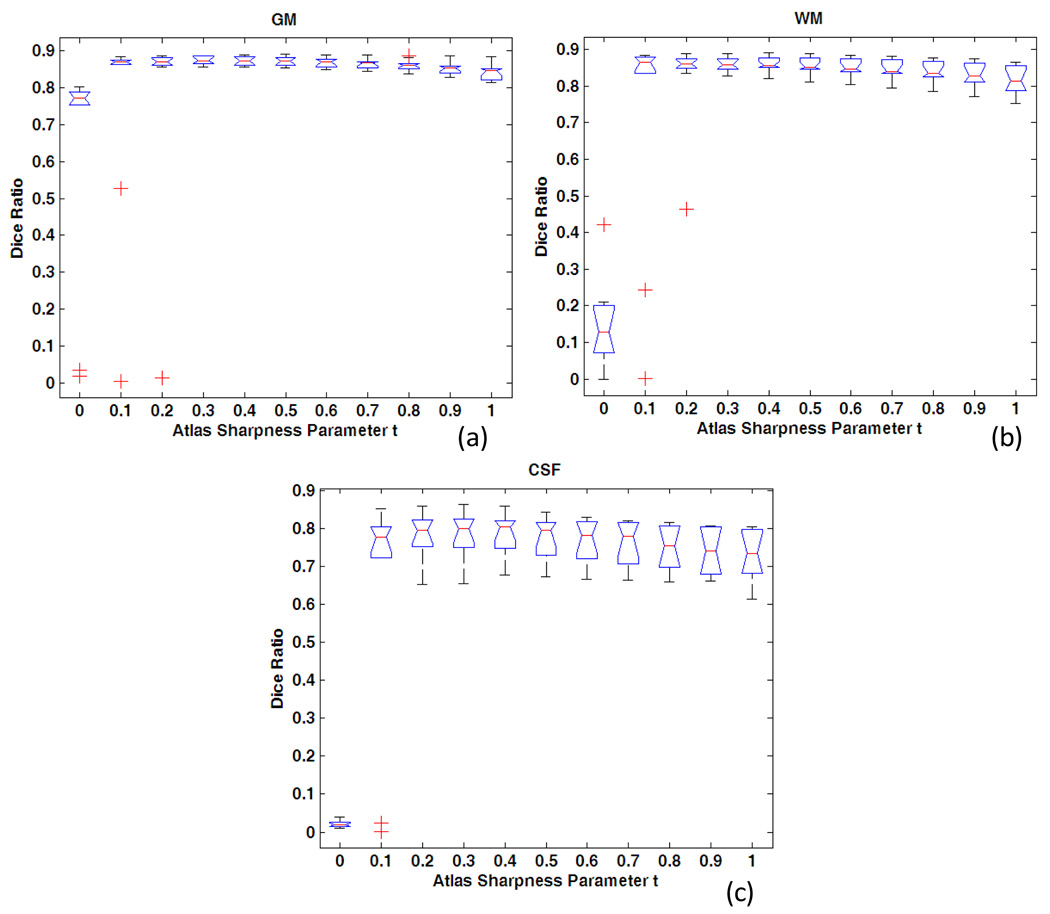
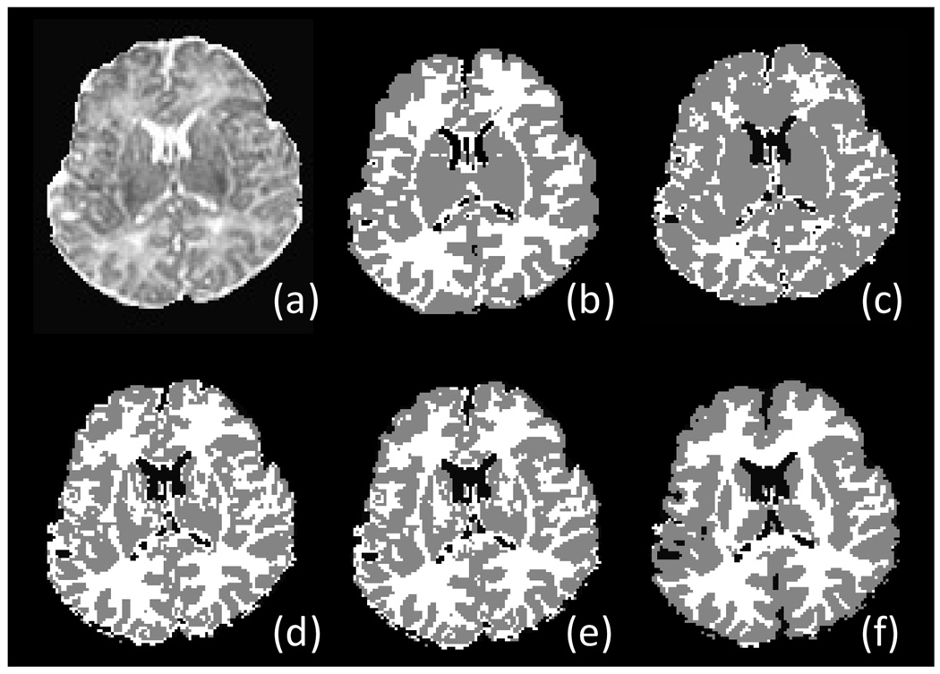
Different sharpness parameter t is chosen from 0 to 1 with interval 0.1 and applied to all 10 subjects, to explore an optimal range for neonatal brain segmentation. The average Dice ratio is shown in Fig. 6. The results indicate that when t is in the range of 0 to 0.2 corresponding to the segmentation with little prior knowledge, the Dice ratio is low and there exist many outliers. The segmentation performance becomes much better when the parameter t is in the range of 0.3 to 1.0. However, as atlas going too strong (i.e., higher percentage) from 0.7 to 1.0, the Dice ratio goes down, reflecting the fact that atlas dominates the segmentation and the image itself contributes little in segmentation. Representative examples for the segmentation results with t in {0,0,3,0,6,1} are shown in Fig. 7. For example, as shown in Fig. 7(c), when a weak atlas is used, the GM is oversegmented. In Fig. 7(f), when a strong atlas is used, the atlas-based segmentaion algoithm can even segment the putamen in subcortical region, where the intensity contrast is actually too low to be differentiated from other nearby tissues in the neonatal T2 image (Fig. 7a). Thus, this causes artifacts in segmentation result.
Fig. 6.
Segmentation accuracy on 10 subjects with respect to the change of atlas sharpness parameter t. The manual segmentation is used as ground truth (rater 1). (a) for GM, (b) for WM, and (c) for CSF.
Fig. 7.
Respentative segmentation results on one subject with respect to the change of atlas sharpness parameter t. (a) Original T2 image, (b) its manual segmentation, and segmentation results using (c) t = 0, (d) t = 0.3, (e) t = 0.6, (f) t = 1 to control the sharpness of the subject-specific atlas in guiding tissue segmentation.
To detemine the trade-off between sharp and blurry atlas used for tissue segmentation, a leave-one-out strategy is also utilized. The total Dice ratios for 9 of 10 subjects are averaged with respect to the change t of, and the parameter t coresponding to the highest accuracy is used for segmentation of the left-out subject. This leave-one-out step is repeated until all subjects have been left out for one time as a test subject. We can eventually obtain a set of optimal t from 10 leave-one-out cases. On the other hand, by testing parameter t independently for each subject as described in the last paragraph and also in Fig. 6, we can obtain an optimal t for each subject, and finally obtain a second set of optimal t from all 10 subjects after they are tested independently. We found that these two sets of t both fall into the range of 0.3–0.6, and no significant difference was found between their corresponding Dice ratios (p=0.32) after performing a paired t-test. This suggests that the optimal parameter t is quite robust across different subjects. Because the segmentation accuracy remains consistent across subjects when t is in the range of 0.3–0.6 as shown in Fig. 6, we set t as 0.5 in this paper for all other experimental results reported below.
Selection of late time-point image
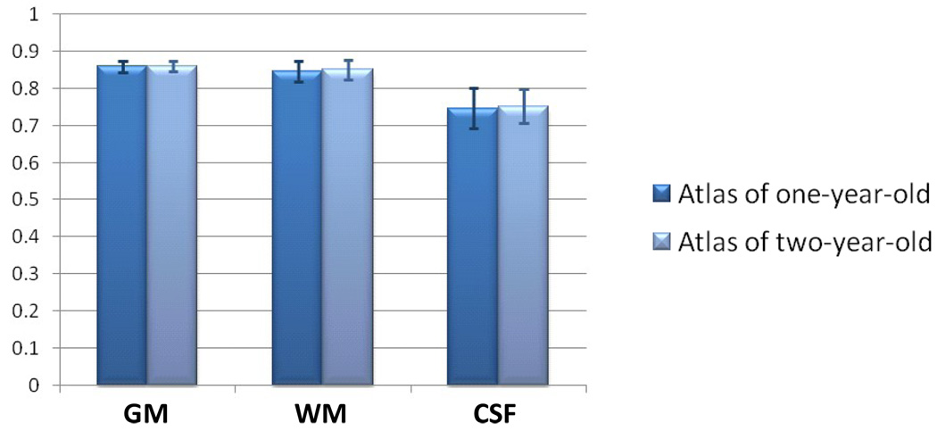
For the four subjects with both one-year-old and two-year-old images, the subject-specific atlas could be built with either one-year-old or two-year-old image. A question rises naturally as which time-point image is more suitable for guiding the neonatal image segmentation. We thus build atlas with either of them and conduct the segmentation separately, with results shown in Fig. 8, to compare their performances. The atlas built by two-year-old image achieves similar performance to that by one-year-old image,. This suggests that both time-point images are able to perform well in the proposed segmentation framework.
Fig. 8.
Similar segmentation performance on GM, WM, and CSF for 4 subjects with atlas built by either one-year-old image or two-year-old image.
Performance evaluation
Visual inspection
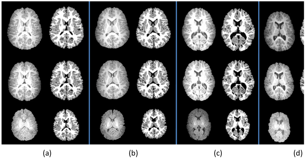
By choosing the optimized atlas sharpness parameter t (i.e., t = 0.5 ) and a proper late time-point image, the segmentation is conducted on all new subjects. The results of 4 representative subjects with three longitudinal scans are shown in Fig. 9 for visual inspection. In each panel from (a) to (d), the first column shows the intensity images and the second column shows the segmentation results. The similar anatomical structures could be observed in intensity images of three time-points for each subject, which are well preserved in their segmented images. These results indicate that the proposed algorithm can obtain visually reasonable segmentation results for neonatal images.
Fig. 9.
Segmentation results of longitudinal images from 4 subjects, corresponding to the panels in (a–d), respectively. For each subject, from top to bottom are the two-year-old, one-year-old, and two-week images, and from left to right are the skull-stripped images and the segmentation results, respectively.
Quantitative comparison with manual segmentations
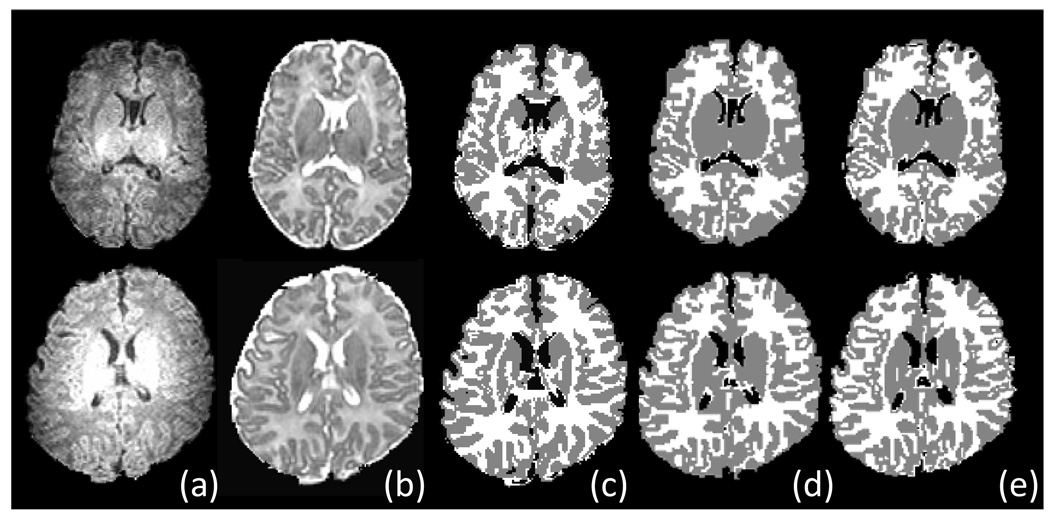
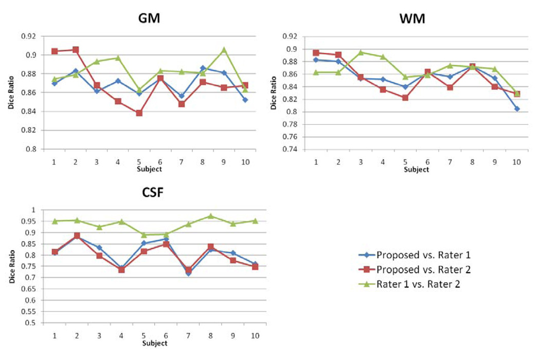
The segmentation results for two representative subjects by our proposed method and by two raters are shown in Fig. 10. These results demonstrate that the proposed algorithm obtained segmentation results visually similar to those generated by expert raters even at fine structures, e.g., cortical regions. The tissue contrast in subcortical regions is quite low (even for manual raters), thus the manual raters leave these regions as gray matter. Accordingly, we mainly compare the segmentation performance in the cortical regions. Fig. 11 shows the Dice ratio for the segmentation results by the proposed segmentation algorithm and the two manual raters. In GM, the Dice ratio is 0.87±0.01 between the proposed algorithm and rater 1, 0.87±0.02 between the proposed algorithm and rater 2, and 0.88±0.01 between two raters. In WM, the Dice ratio is 0.86±0.02 between the proposed algorithm and rater 1, 0.85±0.03 between the proposed algorithm and rater 2, and 0.87±0.02 between two raters. The overlap ratios on GM and WM are very close, and no significant difference was found in each pair of these overlap ratios. Thus, our proposed automatic segmentation algorithm achieved comparable segmentation performance on GM and WM as manual raters. But for CSF, as shown in Fig. 11, the inter-rater overlap rate is much higher as 0.94±0.03 than 0.81±0.05 obtained between the proposed algorithm and rater 1, as well as 0.80±0.05 obtained between the proposed algorithm and rater 2, which may be because the two manual raters used the same initial segmentation as a base for manual edition.
Fig. 10.
Segmentation results of two neonatal images (top and bottom) by our proposed algorithm and two manual raters. (a–b) Original T1 and T2 images, (c) Segmentation results by our proposed algorithm, (d–e) Manual segmentation results by two experts.
Fig. 11.
Comparison of segmentation agreement on GM and WM for 10 subjects between the proposed algorithm and two raters. The inter-rater Dice ratio is also provided.
Quantitative comparison with two population-atlas-based segmentations
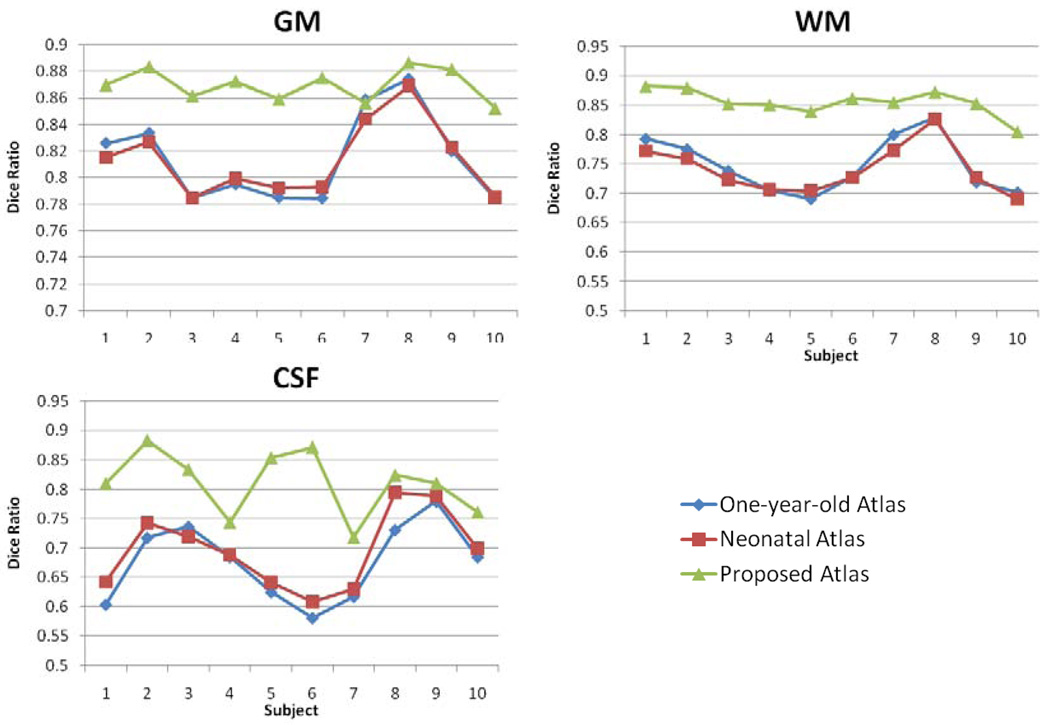
To evaluate the performance of our subject-specific atlas, we compare it with two population atlases. The first one is a one-year-old pediatric atlas obtained from 76 infants with ages ranging from 9 to 15 months (Altaye et al., 2008). The second one is a neonatal atlas, which is built by averaging the normalized segmented images from 9 of 10 neonatal subjects of this study under a leave-one-out strategy. After the step of atlas reconstruction from 9 subjects, the left-out subject is segmented by the reconstructed atlas, to test the atlas performance. This leave-one-out step is repeated until all subjects have been left out for one time as a test subject. For fair comparison, the same joint registration-segmentation strategy is used to segment brain images for our proposed algorithm and these two population-atlas-based segmentation methods. As shown by results in Fig. 12, the proposed algorithm achieved a significant higher Dice ratio in GM, WM, and CSF, compared to the two population-atlas-based methods (with p<0.001). The results by two population-atlas-based segmentation methods are very similar, with no statistically significant difference. Theoretically the neonatal atlas (reconstructed by 9 subjects in the leave-one-out training) should have better performance because it has less anatomical difference from the to-be-segmented neonatal image. The reason that it achieves similar segmentation performance as the one-year-old pediatric atlas might be because the number of neonatal images used for constructing neonatal atlas is too small, i.e., only 9 in this study.
Fig. 12.
Comparison of segmentation accuracy on GM and WM for 10 subjects, using one-year-old atlas, neonatal atlas, and our proposed longitudinal subject-specific atlas, respectively. Manual segmentation from rater 1 is used as ground truth.
Discussion
We have presented a framework for performing neonatal brain tissue segmentation by using a subject-specific tissue probabilistic atlas generated from longitudinal data. This method takes the advantage of longitudinal imaging study in our project, i.e., using the segmentation results of the images acquired at a late time to guide the segmentation of the images acquired at neonatal stage. The experimental results demonstrate that the subject-specific atlas has superior performance, compared to the two population-based atlases, and also the proposed algorithm achieves comparable performance as manual raters in neonate brain image segmentation.
The atlas sharpness parameter has been proved robust for achieving optimal segmentation results in a broad range of 0.3–0.6. For the selection of late time-point image, the segmentation accuracy remains similar when the atlas is built by either one-year-old or two-year-old image. Recently, decision fusion is widely used to combine multiple segmentations into a final decision with compensation for errors in single segmentation (Heckemann et al., 2006; Warfield et al., 2004). This technique could be potentially used to achieve better neonatal segmentation performance, by combining the segmentation results from multiple subject-specific atlases when multiple late time-point images of the same subject are available.
The average total computation time is around 28 minutes for segmentation of a 256×256×198 image with 1×1×1 spatial resolution on a PC with 2.5 GHz Pentium4 processor. Among this computational time, 3 minutes are used for segmentation of a late time-point image for generating a subject-specific atlas, 14 minutes are used for atlas-to-subject registration, and 11 minutes are used for atlas-based neonatal image segmentation. Overall, the proposed segmentation framework is able to achieve satisfactory segmentation results within a reasonable computational time.
The performance of our neonatal segmentation algorithm is currently evaluated by 10 manually segmented subjects. We have acquired a large set of longitudinal images in our institute. In the future, we plan to perform more manual segmentation on more subjects for better evaluating the proposed neonatal segmentation method.
It is worth noting that, by developing this longitudinal guided segmentation algorithm, we can use it to segment more than 180 neonatal images in our database. In this way, using this large set of segmented neonatal images, we can construct a reasonable atlas for neonatal brain images. Eventually, we can use this atlas for segmenting neonatal images with missing longitudinal data. All of these are our ongoing work.
Acknowledgments
This work was supported in part by grants EB006733, EB008760, EB008374, EB009634, NS055754, MH064065, and HD053000.
Footnotes
Publisher's Disclaimer: This is a PDF file of an unedited manuscript that has been accepted for publication. As a service to our customers we are providing this early version of the manuscript. The manuscript will undergo copyediting, typesetting, and review of the resulting proof before it is published in its final citable form. Please note that during the production process errors may be discovered which could affect the content, and all legal disclaimers
References
- Aljabar P, Heckemann RA, Hammers A, Hajnal JV, Rueckert D. Multi-atlas based segmentation of brain images: Atlas selection and its effect on accuracy. NeuroImage. 2009;46:726–738. doi: 10.1016/j.neuroimage.2009.02.018. [DOI] [PubMed] [Google Scholar]
- Altaye M, Holland SK, Wilke M, Gaser C. Infant brain probability templates for MRI segmentation and normalization. NeuroImage. 2008;43:721–730. doi: 10.1016/j.neuroimage.2008.07.060. [DOI] [PMC free article] [PubMed] [Google Scholar]
- Armstrong E, Schleicher A, Omran H, Curtis M, Zilles K. The Ontogeny of Human Gyrification. Cerebral Cortex. 1995;5:56–63. doi: 10.1093/cercor/5.1.56. [DOI] [PubMed] [Google Scholar]
- Ashburner J, Friston KJ. Unified segmentation. NeuroImage. 2005;26:839–851. doi: 10.1016/j.neuroimage.2005.02.018. [DOI] [PubMed] [Google Scholar]
- Bazin PL, Pham DL. Topology-Preserving Tissue Classification of Magnetic Resonance Brain Images. IEEE Transactions on Medical Imaging. 2007;26:487–496. doi: 10.1109/TMI.2007.893283. [DOI] [PubMed] [Google Scholar]
- Bezdek JC, Ehrlich R. FCM: The fuzzy c-means clustering algorithm. Comput. Geosci. 1984;10:191–203. [Google Scholar]
- Cocosco CA, Zijdenbos AP, Evans AC. A fully automatic and robust brain MRI tissue classification method. Med Image Anal. 2003;7:513–527. doi: 10.1016/s1361-8415(03)00037-9. [DOI] [PubMed] [Google Scholar]
- Dice LR. Measures of the Amount of Ecologic Association Between Species. Ecology. 1945;26:297–302. [Google Scholar]
- Dubois J, Benders M, Cachia A, Lazeyras F, Ha-Vinh Leuchter R, Sizonenko SV, Borradori-Tolsa C, Mangin JF, Huppi PS. Mapping the Early Cortical Folding Process in the Preterm Newborn Brain. Cerebral Cortex. 2008;18:1444–1454. doi: 10.1093/cercor/bhm180. [DOI] [PubMed] [Google Scholar]
- Fischl B, Salat DH, Busa E, Albert M, Dieterich M, Haselgrove C, van der Kouwe A, Killiany R, Kennedy D, Klaveness S. Whole Brain Segmentation Automated Labeling of Neuroanatomical Structures in the Human Brain. Neuron. 2002;33:341–355. doi: 10.1016/s0896-6273(02)00569-x. [DOI] [PubMed] [Google Scholar]
- Gerig G, Davis B, Lorenzen P, Xu S, Jomier M, Piven J, Joshi S. Computational Anatomy to Assess Longitudinal Trajectory of Brain Growth. Third International Symposium on 3D Data Processing, Visualization, and Transmission (3DPVT'06); Washington DC, USA; IEEE Computer Society. 2006. pp. 1041–1047. [Google Scholar]
- Heckemann RA, Hajnal JV, Aljabar P, Rueckert D, Hammers A. Automatic anatomical brain MRI segmentation combining label propagation and decision fusion. NeuroImage. 2006;33:115–126. doi: 10.1016/j.neuroimage.2006.05.061. [DOI] [PubMed] [Google Scholar]
- Knickmeyer RC, Gouttard S, Kang C, Evans D, Wilber K, Smith JK, Hamer RM, Lin W, Gerig G, Gilmore JH. A structural MRI study of human brain development from birth to 2 years. J Neurosci. 2008;28:12176–12182. doi: 10.1523/JNEUROSCI.3479-08.2008. [DOI] [PMC free article] [PubMed] [Google Scholar]
- Kwon MJ, Han YJ, Shin IH, Park HW. Hierarchical fuzzy segmentation of brain MR images. International Journal of Imaging Systems and Technology. 2003;13:115–125. [Google Scholar]
- Mewes AUJ, Huppi PS, Als H, Rybicki FJ, Inder TE, McAnulty GB, Mulkern RV, Robertson RL, Rivkin MJ, Warfield SK. Regional brain development in serial magnetic resonance imaging of low-risk preterm infants. Pediatrics. 2006;118:23–33. doi: 10.1542/peds.2005-2675. [DOI] [PubMed] [Google Scholar]
- Nishida M, Makris N, Kennedy DN, Vangel M, Fischl B, Krishnamoorthy KS, Caviness VS, Grant PE. Detailed semiautomated MRI based morphometry of the neonatal brain: preliminary results. NeuroImage. 2006;32:1041–1049. doi: 10.1016/j.neuroimage.2006.05.020. [DOI] [PubMed] [Google Scholar]
- Pham D, Prince JL, Xu C, Dagher AP. An automated technique for statistical characterization of brain tissues in magnetic resonance imaging. International journal of pattern recognition and artificial intelligence. 1997;11:1189–1212. [Google Scholar]
- Pham DL, Prince JL. An adaptive fuzzy C-means algorithm for image segmentation in the presence of intensity inhomogeneities. Pattern Recognition Letters. 1999;20:57–68. [Google Scholar]
- Pham DL, Xu C, Prince JL. A survey of current methods in medical image segmentation. Annual Review of Biomedical Engineering. 2000;2:315–337. doi: 10.1146/annurev.bioeng.2.1.315. [DOI] [PubMed] [Google Scholar]
- Pohl KM, Fisher J, Grimson WEL, Kikinis R, Wells WM. A Bayesian model for joint segmentation and registration. NeuroImage. 2006;31:228–239. doi: 10.1016/j.neuroimage.2005.11.044. [DOI] [PubMed] [Google Scholar]
- Prastawa M, Gilmore JH, Lin W, Gerig G. Automatic segmentation of MR images of the developing newborn brain. Med Image Anal. 2005;9:457–466. doi: 10.1016/j.media.2005.05.007. [DOI] [PubMed] [Google Scholar]
- Rohlfing T, Russakoff DB, Maurer CR. IPMI 2003. Springer; 2003. Expectation maximization strategies for multi-atlas multi-label segmentation; pp. 210–221. [DOI] [PubMed] [Google Scholar]
- Shattuck DW, Leahy RM. Automated graph-based analysis and correction of cortical volume topology. IEEE Trans Med Imaging. 2001;20:1167–1177. doi: 10.1109/42.963819. [DOI] [PubMed] [Google Scholar]
- Shen D, Davatzikos C. HAMMER: hierarchical attribute matching mechanism for elastic registration. IEEE Trans Med Imaging. 2002;21:1421–1439. doi: 10.1109/TMI.2002.803111. [DOI] [PubMed] [Google Scholar]
- Sled JG, Zijdenbos AP, Evans AC. A nonparametric method for automatic correction of intensity nonuniformity in MRI data. IEEE Trans Med Imaging. 1998;17:87–97. doi: 10.1109/42.668698. [DOI] [PubMed] [Google Scholar]
- Smith SM. Fast robust automated brain extraction. Human Brain Mapping. 2002;17:143–155. doi: 10.1002/hbm.10062. [DOI] [PMC free article] [PubMed] [Google Scholar]
- Song Z, Awate SP, Licht DJ, Gee JC. Clinical neonatal brain MRI segmentation using adaptive nonparametric data models and intensity-based Markov priors. MICCAI 2007. 2007:883–890. doi: 10.1007/978-3-540-75757-3_107. [DOI] [PubMed] [Google Scholar]
- Thomas Yeo BT, Sabuncu MR, Desikan R, Fischl B, Golland P. Effects of registration regularization and atlas sharpness on segmentation accuracy. Med Image Anal. 2008 doi: 10.1016/j.media.2008.06.005. [DOI] [PMC free article] [PubMed] [Google Scholar]
- Van Leemput K, Maes F, Vandermeulen D, Suetens P. Automated model-based bias field correction of MR images of the brain. IEEE Trans Med Imaging. 1999;18:885–896. doi: 10.1109/42.811268. [DOI] [PubMed] [Google Scholar]
- Wang F, Vemuri BC, Eisenschenk SJ. Joint registration and segmentation of neuroanatomic structures from brain MRI. Academic radiology. 2006;13:1104–1111. doi: 10.1016/j.acra.2006.05.017. [DOI] [PMC free article] [PubMed] [Google Scholar]
- Warfield SK, Kaus M, Jolesz FA, Kikinis R. Adaptive, template moderated, spatially varying statistical classification. Med Image Anal. 2000;4:43–55. doi: 10.1016/s1361-8415(00)00003-7. [DOI] [PubMed] [Google Scholar]
- Warfield SK, Zou KH, Wells WM. Simultaneous truth and performance level estimation (STAPLE): an algorithm for the validation of image segmentation. IEEE Trans Med Imaging. 2004;23:903–921. doi: 10.1109/TMI.2004.828354. [DOI] [PMC free article] [PubMed] [Google Scholar]
- Weisenfeld NI, Warfield SK. Automatic segmentation of newborn brain MRI. NeuroImage. 2009;47:564–572. doi: 10.1016/j.neuroimage.2009.04.068. [DOI] [PMC free article] [PubMed] [Google Scholar]
- Xue H, Srinivasan L, Jiang S, Rutherford M, Edwards AD, Rueckert D, Hajnal JV. Automatic segmentation and reconstruction of the cortex from neonatal MRI. NeuroImage. 2007;38:461–477. doi: 10.1016/j.neuroimage.2007.07.030. [DOI] [PubMed] [Google Scholar]
- Yeo BTT, Sabuncu MR, Desikan R, Fischl B, Golland P. Effects of registration regularization and atlas sharpness on segmentation accuracy. Med Image Anal. 2008:603–615. doi: 10.1016/j.media.2008.06.005. [DOI] [PMC free article] [PubMed] [Google Scholar]
- Yezzi A, Zollei L, Kapur T. A variational framework for integrating segmentation and registration through active contours. Med Image Anal. 2003;7:171–185. doi: 10.1016/s1361-8415(03)00004-5. [DOI] [PubMed] [Google Scholar]
- Yushkevich PA, Piven J, Hazlett HC, Smith RG, Ho S, Gee JC, Gerig G. User-guided 3D active contour segmentation of anatomical structures: Significantly improved efficiency and reliability. NeuroImage. 2006;31:1116–1128. doi: 10.1016/j.neuroimage.2006.01.015. [DOI] [PubMed] [Google Scholar]


