Thermodynamic properties of liquid water: an application of a nonparametric approach to computing the entropy of a neat fluid

Abstract

Due to its fundamental importance to molecular biology, great interest has continued to persist in developing novel techniques to efficiently characterize the thermodynamic and structural features of liquid water. A particularly fruitful approach, first applied to liquid water by Lazaridis and Karplus, is to use molecular dynamics or Monte Carlo simulations to collect the required statistics to integrate the inhomogeneous solvation theory equations for the solvation enthalpy and entropy. We here suggest several technical improvements to this approach, which may facilitate faster convergence and greater accuracy. In particular, we devise a nonparametric k’th nearest neighbors (NN) based approach to estimate the water-water correlation entropy, and suggest an alternative factorization of the water-water correlation function that appears to more robustly describe the correlation entropy of the neat fluid. It appears that the NN method offers several advantages over the more common histogram based approaches, including much faster convergence for a given amount of simulation data; an intuitive error bound that may be readily formulated without resorting to block averaging or bootstrapping; and the absence of empirically tuned parameters, which may bias the results in an uncontrolled fashion.

1 Introduction

Water is unique among liquids for its biological significance. It plays an active role in the formation of the structures of proteins, lipid bilayers, and nucleic acids in vivo, both through direct hydrogen bonding interactions with these biomolecules, and also through indirect interactions, where the unique hydrogen-bonded structure of liquid water is known to drive hydrophobic assembly.¹ It has been suggested that a robust characterization of the thermodynamic properties and structure of water solvating the active site of a protein is essential to rationalize the various binding affinities of small molecules that will displace that solvent to bind to the protein active site.^2,3

As such, great interest has continued to persist in developing novel techniques to efficiently characterize the thermodynamic and structural features of liquid water in different environments. A particularly fruitful approach, first applied to liquid water by Lazaridis and Karplus,^4–6 used molecular dynamics or Monte Carlo simulations to collect the required statistics to integrate the inhomogeneous solvation theory (IST) equations for the solvation enthalpy and entropy. In this theory, the solvation enthalpy is determined from an analysis of the change in the solute-solvent and solvent-solvent interaction energy terms, and the solvation entropy is computed from an expansion of the entropy in terms of increasingly higher order solute-solvent correlation functions.⁴ This approach has been used to characterize the thermodynamics and structure of neat water,⁶ hydration of small hydrophobes,⁴ and the hydration of the active sites of proteins.^7,8 Recently, it has also been extended to allow for the rapid computation of the relative binding affinities of a set of congeneric ligands with a given protein, via a semi-empirical displaced-solvent functional.²

Due to the increasing interest in applying this technique to water^9–12 in various environments, we have chosen to reexamine the factorization and correlation function integration scheme originally suggested by Lazaridis and Karplus⁶ for bulk water and later adopted by others.¹³ We have found that several technical improvements in this scheme are possible, which may facilitate faster convergence and greater accuracy than the more typical expressions. In this paper, we (1) devise a nonparametric k’th nearest neighbors (NN)¹⁴ based approach to estimate the water-water correlation entropy, in lieu of the more common histogram based approaches; and (2) suggest an alternative factorization for the water-water correlation function that appears to more robustly describe the water-water correlation entropy of the neat fluid. To our knowledge, this is the first application of the NN method to compute the entropy of a neat fluid. It appears that the NN method offers several advantages over the more common histogram based approaches, including (1) much faster convergence for a given amount of simulation data, especially when the correlation function is highly structured; (2) an intuitive error bound may be readily formulated without resorting to block averaging or bootstrapping techniques, which may be problematic to apply to estimators of the entropy; and (3) the absence of empirically tuned parameters, such as the histogram bin width, which may bias the results in an unpredictable fashion. Our alternative factorization of the water-water correlation function explicitly includes correlations between the water-dipole-vector-intermolecular-axis angle with the angle of rotation of the water molecule about its dipole vector. This contribution, although neglected by others,⁶ has been found in our work to increase the agreement of results obtained by the entropy expansion with those obtained by less approximate methods, such as free energy perturbation theory. We also extensively compare the solvation entropies obtained from the truncated entropy expansion to those obtained from a finite difference analysis of free energy perturbation theory results. This comparison allows us to characterize the errors in both precision and accuracy associated with the NN method of integrating the entropy expansion presented here.

Our primary interest in developing this technique was to later adapt the method to study the solvation of solutes; thus, we were interested in determining realistic estimates of the convergence of the technique when the isotropic symmetry of the fluid was not present. As such, when extracting the solvent configurations to compute the pair correlation function (PCF), we chose to use only the configurations of a distinguished solvent molecule with the rest of the system, instead of collecting statistics from all pairs of solvent molecules. Such a protocol allows for an interrogation of the relative convergence properties of the various methods that might be obscured by the additional statistics offered by taking advantage of the symmetry of the system.

2 Methods

2.1 The Entropy expression of a neat fluid

First derived by Green,¹⁵ and later by Raveché¹⁶ and Wallace,¹⁷ the entropy of a fluid can be expressed as a sum of integrals over multi-particle correlation functions. For a molecular fluid,⁵ the expression is

$$\begin{array}{cc}s=\hfill & s^{\mathit{\text{id}}}+s_e=s^{\mathit{\text{id}}}-\frac{1}{2!}k\frac{\rho }{{\mathrm{\Omega }}^2}{\displaystyle \int [g^{(2)}\text{ln}\left(g^{(2)}\right)-g^{(2)}+1]d\mathbf{r}d{\mathbf{\omega }}^2}\hfill \\ & -\frac{1}{3!}k\frac{{\rho }^2}{{\mathrm{\Omega }}^3}{\displaystyle \int [g^{(3)}\text{ln}\left(\delta g^{(3)}\right)-g^{(3)}+3g^{(2)}{g}^{(2)}-3g^{(2)}+1]d{\mathbf{r}}_{\mathbf{1}}d{\mathbf{r}}_{\mathbf{2}}d{\omega }^3–\cdots }\hfill \end{array}$$ (1)

where, s^id is the entropy of an ideal gas with the same density and temperature as the fluid, s_e is the excess entropy of the fluid over that of the ideal gas, k is the Boltzmann’s constant, and ρ is the number density, ω denotes the orientational variables of one molecule, Ω is the total volume of the orientational space (For nonlinear molecule like water, Ω is 8π²), g⁽²⁾ is the pair correlation function, g⁽³⁾ is the triplet correlation function, and δg⁽³⁾ is the deviation of g⁽³⁾ from the superposition approximation. In practice, it is very difficult or even impossible to converge the three-particle and higher order correlation terms. However, it has been established that, for most fluids, the largest contribution to the excess entropy comes from the two-particle correlation term,⁶ and the error induced by neglecting the higher order terms of the expansion may often be safely ignored.

Following the work of Lazaridis and Karplus,⁶ we evaluate the two-particle excess entropy of liquid water by separating the two-particle term into translational and orientational components by factorization:

$$g(r,{\omega }^2)=g(r)g({\omega }^2|r)$$ (2)

$$s_e^{(2)}=s_{\mathit{\text{trans}}}^{(2)}+s_{\mathit{\text{orient}}}^{(2)}$$ (3)

$$s_{\mathit{\text{trans}}}^{(2)}=-\frac{1}{2}k\rho {\displaystyle \int [g(r)\text{ln}g(r)-g(r)+1]d\mathbf{r}}$$ (4)

$$s_{\mathit{\text{orient}}}^{(2)}=\frac{1}{2}k\rho {\displaystyle \int g(r)S^{\mathit{\text{orient}}}(r)d\mathbf{r}}$$ (5)

$$S^{\mathit{\text{orient}}}=-\frac{1}{{\mathrm{\Omega }}^2}{\displaystyle \int J({\omega }^2)g({\omega }^2|r)\text{ln}g({\omega }^2|r)d{\omega }^2}$$ (6)

where r is the Oxygen-Oxygen distance of two water molecules, ω² are the angles that define the relative orientation of the two water molecules, J(ω²) is the Jacobian of the angular variables, g(r, ω²) is the pair correlation function, and g(ω²|r) is the conditional-angular pair correlation function in the typical Bayesian notion. (Note that g(r, ω²) is identical to g⁽²⁾ as it appears in equation 1.) We denote the relative orientation of the two water molecules by the five angles⁶ [θ₁,θ₂,ϕ,χ₁,χ₂], where θ₁,θ₂ are the angles between the intermolecular axis and the dipole vector of each molecule, ϕ describes the relative dihedral rotation of the dipole vector around the intermolecular axis, and χ₁,χ₂ describe the rotation of each molecule around its dipole vector. In the following discussion, we denote the entropy defined by formula 6 the orientational Shannon entropy,¹⁸ and denote the entropy defined by formula 5 the orientational excess entropy.

In line with prior work,⁶ we calculated the orientational Shannon entropy as defined by formula 6 for three different ranges of r: (0 < r ≤ 2.7), (2.7 < r ≤ 3.3), and (3.3 < r ≤ 5.6), which correspond to the various peaks and troughs in the radial distribution function. In this way, the orientational excess entropy is related to Shannon entropy by:

$$s_{\mathit{\text{orient}}}=\frac{1}{2}{N}_{i}k{S}^{\mathit{\text{orient}}}\mathrm{i}=1,2,3$$ (7)

where N_i is the average number of water molecules in the i-th shell.

2.2 Factorization of the orientational pair correlation function using generalized Kirkwood superposition approximation

The orientational pair correlation function (PCF) of water is a function of five angles, which is very difficult to converge from currently accessible molecular dynamics simulation time scales. The idea of factorization is to approximate the higher dimensional probability density function by the product of its lower dimensional marginal probability density functions. The generalized Kirkwood superposition approximation (GKSA),^19–21 allows an m-dimensional distribution to be estimated using corresponding m-1-dimensional distributions:

$$\rho (x_1,x_2,\cdots ,x_m)=\{\begin{array}{c}\frac{{\displaystyle \prod _{c_{m-1}^m}{\rho }_{m-1}\cdots }{\displaystyle \prod _{c_2^m}{\rho }_2}}{{\displaystyle \prod _{c_{m-2}^m}{\rho }_{m-2}\cdots }{\displaystyle \prod _{c_1^m}{\rho }_1}}\text{ m is odd}\\ \frac{{\displaystyle \prod _{c_{m-1}^m}{\rho }_{m-1}\cdots }{\displaystyle \prod _{c_1^m}{\rho }_1}}{{\displaystyle \prod _{c_{m-2}^m}{\rho }_{m-2}\cdots }{\displaystyle \prod _{c_2^m}{\rho }_2}}\text{ m is even}\end{array}$$ (8)

where ρ_m−k represents a specific probability density function of m − k dimensionality, and $c_{m-k}^m$ indicates all possible combinations of m − k groupings from the set of m total variables. Reiss²⁰ and Singer²¹ have demonstrated that the GKSA is the optimal approximation of an n-particle distribution for n ≥ 3 from a variational point of view, and it has been applied in numerous settings.^22,23

From the results of our simulations, and as indicated by Lazaridis and Karplus,⁶ the distribution has no structure along angleϕ, i.e. g(ϕ) is close to 1 over the range of ϕ, and has no correlation with other angles. Thus, we approximated the 5 dimensional PCF by:

$$g({\theta }_1,{\theta }_2,\varphi ,{\chi }_1,{\chi }_2)=g({\theta }_1,{\theta }_2,{\chi }_1,{\chi }_2)g(\varphi )$$ (9)

Note that for any properly defined orientational PCF g(x₁,x₂⋯x_N),

$$\frac{1}{{\mathrm{\Omega }}^{[x_1,x_2\cdots x_n]}}{\displaystyle \int J(x_1,x_2\cdots x_n)g(x_1,x_2\cdots x_n)d{x}_{1}d{x}_2\cdots d{x}_n=1}$$ (10)

where

$${\mathrm{\Omega }}^{[x_1,x_2\cdots x_n]}={\displaystyle \int J(x_1,x_2\cdots x_n)d{x}_{1}d{x}_2\cdots d{x}_n}$$ (11)

i.e., Ω^{[x₁,x₂⋯x_n]} is the integral of the Jacobian J(x₁,x₂⋯x_n) over angular variables x₁,x₂⋯x_n. Therefore, g(x₁,x₂⋯x_n) is proportional to ρ(x₁,x₂⋯x_n) with proportional coefficient Ω^{[x₁,x₂⋯x_n]}. Via application of the GKSA (formula 8), it follows

$$g({\theta }_1,{\theta }_2,{\chi }_1,{\chi }_2)=\frac{g({\theta }_1,{\theta }_2)g({\theta }_1,{\chi }_1)g({\theta }_1,{\chi }_2)g({\theta }_2,{\chi }_1)g({\theta }_2,{\chi }_2)g({\chi }_1,{\chi }_2)}{g^2({\theta }_1)g^2({\theta }_2)g^2({\chi }_1)g^2({\chi }_2)}$$ (12)

Note that this factorization differs from that introduced by Karplus and Lazaridis⁶ by the explicit inclusion of g(θ₁,χ₁) and g(θ₂,χ₂) terms. Taking this approximation of g(x₁,x₂⋯x_n) into the argument of the logarithm of formula 6 we find

$$S^{\mathit{\text{orient}}}=-\frac{1}{{\mathrm{\Omega }}^2}{\displaystyle \int J({\omega }^2)g({\omega }^2|r)\text{ln}g({\omega }^2|r)d{\omega }^2}$$ (13)

$$\begin{array}{c}=-{\displaystyle \sum _{C_2^4}\frac{1}{{\mathrm{\Omega }}^{[x_1,x_2]}}{\displaystyle \int J(x_1,x_2)g(x_1,x_2)\text{ln}g(x_1,x_2)d{x}_{1}d{x}_2}}\hfill \\ +2{\displaystyle \sum _{C_1^4}\frac{1}{{\mathrm{\Omega }}^{[x]}}{\displaystyle \int J(x)g(x)\text{ln}g(x)\mathit{\text{dx}}}}\hfill \end{array}$$ (14)

$$={\displaystyle \sum _{C_2^4}{S}^{[x_1,x_2]}}-2{\displaystyle \sum _{C_1^4}{S}^{[x]}}$$ (15)

where x₁,x₂ is any combination of two variables from the [θ₁,θ₂,χ₁,χ₂] set, x is any variable from the [θ₁,θ₂,χ₁,χ₂] set, J(x₁,x₂) is the Jacobian of the corresponding two variables, and J(x) is the Jacobian corresponding to variable x, Ω^[x₁,x₂] is the total accessible angular volume of variables x₁,x₂, and Ω^[x] is the total accessible angular volume of variable x, S^[x₁,x₂] is the Shannon entropy of angular variables x₁ and x₂, and S^[x] is the Shannon entropy of angular variable x.

We note that an ambiguity seems to exist in the literature as to how to properly apply an approximation of the type suggested in equation 12 to equation 6. We have adopted here to apply the approximation only to the logarithm of equation 6 (as was done in the original derivation of equation 1), which allows result 15 to be interpreted through the language of information theory.²⁴ An alternate approach, that has been adopted by others, has been to apply approximation 12 to both occurrences of the PCF in equation 6, taking care to renormalize the factorization of the PCF introduced in equation 12 so that meaningful results will still be obtained. Interestingly, the results of these two approaches do not numerically agree, which may not be obvious from cursory inspection. We leave this proof as an exercise for the reader, which can be readily shown for instance from a correlated multidimensional Gaussian distribution.

2.3 The k’th nearest-neighbor method

The NN method¹⁴ gives an asymptotically unbiased estimate of an integral of the form:

$$I=-{\displaystyle \int \rho (x_1,x_2,\cdots ,x_s)\text{ln}\rho (x_1,x_2,\cdots ,x_s)d{x}_{1}d{x}_2\cdots d{x}_s}$$ (16)

where ρ (x₁,x₂,⋯,x_s) is the probability density function. Given a reasonable estimation of probability density function f(xⁱ), the value of integral can be approximated as

$$I\approx -\frac{1}{n}{\displaystyle \sum _{i=1}^n\text{ln}f(x^i)}$$ (17)

which follows from xⁱ being sampled from the true distribution ρ (xⁱ). The NN method of nonparametrically estimating f(xⁱ) at a point $x^i=(x_1^i,x_2^i\cdots ,x_s^i)$ is²⁵

$$f(x^i)=\frac{k}{n}\frac{1}{V_S(R_{i,k})}$$ (18)

$$V_S(R_{i,k})=\frac{{\pi }^{s/2}{R}_{i,k}^s}{\mathrm{\Gamma }(\frac{1}{2}s+1)}$$ (19)

where n is the number of data points in the sample, V_s(R_i,k) is the volume of an s-dimensional sphere with radius R_i,k, and R_i,k is the Euclidean distance between the point xⁱ and its k-th nearest neighbor in the sample. This approximation amounts to assuming that the distance between neighboring sampled points in configuration space will be small where the probability density function is large, and vice versa. So this integration may be estimated as

$$I\approx -\frac{1}{n}{\displaystyle \sum _{i=1}^n\text{ln}f(x^i)}=\frac{1}{n}{\displaystyle \sum _{i=1}^n\text{ln}\frac{n{\pi }^{s/2}{R}_{i,k}^s}{k\mathrm{\Gamma }(\frac{1}{2}s+1)}}$$ (20)

However, the estimate in equation 20 is systematically biased¹⁴ and will deviate from the correct result in the limit of large n by L_k−1 − lnk − γ, where $L_j={\displaystyle {\sum }_{i=1}^j\frac{1}{i}}$ and γ = 0.5772⋯ is Euler’s constant. By subtracting the bias L_k−1 − lnk − γ, the modified unbiased estimate is formulated as

$$I\approx \frac{s}{n}{\displaystyle \sum _{i=1}^n\text{ln}{R}_{i,k}}+\text{ln}\frac{n{\pi }^{s/2}}{\mathrm{\Gamma }(\frac{1}{2}s+1)}-L_{k-1}+\gamma$$ (21)

Now our goal is to modify our expressions for the Shannon entropies into a form that is amenable to a k’th NN evaluation of the integral. The expression of the two-dimensional orientational Shannon entropy has the form of

$$S^{[x_1,x_2]}=-\frac{1}{{\mathrm{\Omega }}^{[x_1,x_2]}}{\displaystyle \int J(x_1,x_2)g(x_1,x_2)\text{ln}g(x_1,x_2)d{x}_{1}d{x}_2}$$ (22)

where J(x₁,x₂) is the Jacobian associated with x₁ and x₂. Here, for χ₁ and χ₂ the Jacobian is 1, but for θ₁ and θ₂ the Jacobian is sin θ₁ and sin θ₂. However, by a change of variables from θ to $t=\frac{\pi }{2}(\text{cos}\theta +1)$, the Jacobian for t becomes 1, and the total angular volume is π for one dimensional distribution and π² for two dimensional distributions. Then, g(x₁,x₂) is proportional to ρ (x₁,x₂) in equation 16, with proportional coefficient π². Following the NN method, the statistically unbiased estimation of the one and two-dimensional orientational Shannon entropies may now be approximated as

$$H_k^{[x]}(n)=\frac{1}{n}{\displaystyle \sum _{i=1}^n\text{ln}{R}_{i,k}}+\text{ln}\frac{n{\pi }^{1/2}}{\mathrm{\Gamma }(\frac{1}{2}+1){\mathrm{\Omega }}^{[x]}}-L_{k-1}+\gamma$$ (23)

$$H_k^{[x_1,x_2]}(n)=\frac{2}{n}{\displaystyle \sum _{i=1}^n\text{ln}{R}_{i,k}}+\text{ln}\frac{n{\pi }^1}{\mathrm{\Gamma }(\frac{1}{2}\times 2+1){\mathrm{\Omega }}^{[x_1,x_2]}}-L_{k-1}+\gamma$$ (24)

where $H_k^{[x]}$ (n)is the k’th NN estimate of the Shannon entropy of random variable x from a sampling of n data points and $H_k^{[x_1,x_2]}$ (n)is the k’th NN estimate of the joint Shannon entropy of random variables x₁,x₂ from a sampling of n data points. Thus, we are now equipped to apply the NN method of estimating the entropy to liquid state problems. We also note that to compute the NN distances, we made use of the ANN code,²⁶ which utilizes the k-d tree algorithm²⁷ for obtaining the k-th NN distances R_i,k between sample points as necessary.

2.4 Error analysis of the k’th nearest neighbor method

It has been shown through an analysis of the limiting distribution¹⁴ that the variance of the k-th NN estimate of the entropy H_k(n) is

$$\mathit{\text{Var}}[H_k(n)]=\frac{Q_k+\mathit{\text{Var}}[\text{ln}f(x)]}{n}$$ (25)

where f(x) is the probability density function and $Q_k={\displaystyle {\sum }_{j=k}^{\mathrm{\infty }}\frac{1}{j^2}}$. Formally, this result follows from using the Poisson approximation of the binomial distribution to characterize the fluctuations of H_k(n) in the large n limit (please see ref.14 for details). Since H_k(n) is asymptotically unbiased,¹⁴ the asymptotic mean square error of the estimate is of the order given by equation 25. Typically, the true value H(n) will be estimated by computing H_k(n) for several values of k, typically 1 to 5. Since the analytical form of the variance is known, we may combine these estimates by a weighted averaging procedure, i.e. H(n) = Σw_kH_k(n). For independent variables with the same average, the weight which minimizes the variance of the estimate of the average is a weight proportional to the inverse of the variance of the variable (see the appendices A for details), i.e.,

$$w_k=\frac{1/(Q_k+\mathit{\text{Var}}[\mathit{\text{ln}}f(x)])}{{\displaystyle {\sum }_{i=1}^{m}1/(Q_k+\mathit{\text{Var}}[\mathit{\text{ln}}f(x)])}}\text{ for}k=1,2,\cdots m$$ (26)

where w_k is the ideal weight of H_k(n) when averaging H(n). Such calculations may also be readily extended to compute the standard deviation of such an estimate (appendices A). Interestingly, two well defined limits exist here: (1) if Var[ln f(x)] is small, then the proper weighting will be

$$w_k=\frac{1/Q_k}{{\displaystyle {\sum }_{k=1}^{m}1/Q_k}}\text{ for}k=1,2\cdots m$$ (27)

and, (2) if Var[ln f(x)] is large, then the proper weighting will be a flat function which will lead to a simple arithmetic average. Therefore, the best possible estimate of H(n) from m estimates of H_k(n) will always be bound by these two limiting averages. Further, if these two limiting averages converge in the given sampling, it is highly probable the estimate of H(n) is also converged. We also note here that an intuitive sense of which regime best fits the given data can be discerned by inspecting the relative noise in plots of the m H_k(n) estimates as a function of n (where n is the amount of simulation time in this application). If the H₁(n) estimate noticeably suffers greater fluctuations than the other estimates, then the Var[ln f(x)] term must be small, since the Q₁ component is dominating relative variances of the estimates. However, if the m H_k(n) estimates all appear graphically to have fluctuations of a similar magnitude, then the Var[ln f(x)] term must be large, and the simple arithmetic average is more appropriate. Such inspection of our data revealed Var[ln f(x)] to be small. As such, the weighted average determined by application of eqn 27 was taken in this work as our best possible estimate of H(n).

2.5 Calculation of the excess energy, enthalpy, and free energy

The excess molar energy of a fluid is simply

$$\mathrm{\Delta }E=\frac{1}{2}\frac{\rho }{{\mathrm{\Omega }}^2}{\displaystyle \int g(r,{\omega }^2)u(r,{\omega }^2)d\mathbf{r}d{\omega }^2}$$ (28)

where u(r, ω²) is the interaction energy between two molecules with distance r and orientation determined by ω². This quantity is straight forward to extract from the simulation, as it is merely one half of the interaction energy between the water molecule of interest with the rest of the system. The molar excess enthalpy can be obtained by approximating the Δ(PV) term. For the liquid phase, the PV term may be safely neglected, and for the gas phase, we may use the ideal gas equation of state PV = NkT to derive an excellent approximation to the PV term analytically. Combined with the excess entropy, we find the excess free energy of the fluid may be expressed as

$$\mathrm{\Delta }G=\mathrm{\Delta }E+\mathrm{\Delta }(\mathit{\text{PV}})-T{s}_e$$ (29)

as is typical.

2.6 The finite-difference method of entropy calculation

In order to generate reference data to examine the accuracy of the k’th NN method of evaluating the entropy expansion, we pursued a finite difference analysis of the solvation free energy, as computed from free energy perturbation theory (FEP). The finite-difference (FD) method of computing an entropy from FEP data proceeds by first noting that the entropy is the temperature derivative of the free energy, and then attempting to accurately estimate this slope,²⁸ ie

$$-\mathrm{\Delta }S(T)={\langle \frac{\partial \mathrm{\Delta }G}{\partial T}\rangle }_P=\frac{\mathrm{\Delta }G(T+\mathrm{\Delta }T)-\mathrm{\Delta }G(T-\mathrm{\Delta }T)}{2\mathrm{\Delta }T}$$ (30)

This method relies on the assumption that the heat capacity of the system is independent of temperature in the range [T − ΔT, T + ΔT].²⁹ This assumption appears to be valid near room temperature with ΔT even as large as 50K.²⁸ Here, we use the Bennett acceptance ratio³⁰ method to calculate the excess free energy of liquid water at T = 298 ± 20K, and then use FD to calculate the excess entropy at T = 298K. The datails of this method are included in the appendices. This data allows for independent validation of the NN approach and the approximations therein.

2.7 Details of the simulation

Dynamics trajectories were generated using the Desmond molecular dynamics program.³¹ A 25 Å cubic box of the TIP4P³² water model was first equilibrated to 298K and 1 atm with Nose-Hoover^33,34 temperature and Martyna-Tobias-Klein³⁵ pressure controls, followed by 30 ns NVT dynamics simulation with a Nose-Hoover^33,34 temperature control. In order to integrate the equations of motion of the system, the RESPA³⁶ integrator was used, where the integration step was 2 fs for the bonded and the nonbonded-near interactions and 6 fs for the nonbonded-far interactions. Configurations were collected every 1.002 ps. The cut-off distance was 9 Å for the Van der Waals interaction, and the particle-mesh Ewald³⁷ method was used to model the electrostatic interactions. Similar simulations were performed for the SPC,³⁸ SPC/E,³⁹ TIP3P³² and TIP4P-Ew⁴⁰ water models.

When extracting the solvent configurations to compute the PCF, we chose to only use the configurations of a distinguished solvent molecule with the rest of the system, instead of collecting statistics from all pairs of solvent molecules. Our primary interest in developing this technique was to later adapt the method to study the solvation of solutes; thus, we were interested in determining realistic estimates of the convergence of the technique when the isotropic symmetry of the fluid was not present. Such a protocol allows for an interrogation of the relative convergence properties of the various methods that might be obscured by the additional statistics offered by taking advantage of the symmetry of the system.

3 Results and discussion

3.1 The Shannon entropies

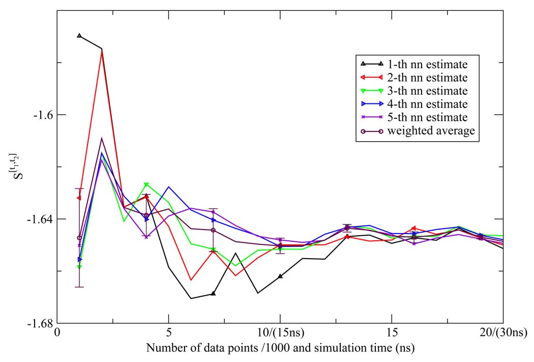
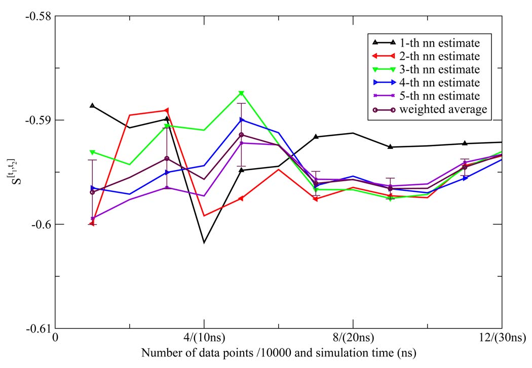
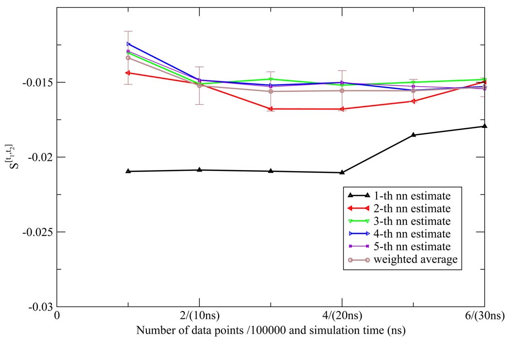
The NN estimates of the two dimensional orientational Shannon entropies S^[t₁,t₂] of the TIP3P water model for the three shells are given in Figure 1, Figure 2, and Figure 3. The results reported in these figures were generally representative of those results obtained for the other models. We see from the figures that the weighted average estimate of all the Shannon entropies are converged over the course of the simulations. The results of all the one and two dimensional orientational Shannon entropies for each of the three shells for all the water models studied are given in Table 1. By application of formula 4 and 7, we computed the translational excess entropies and orientational excess entropies for all the water models studied. All the final results are shown in Table 2. From the table, we see that for the TIP4P model the excess entropy result from the NN method −13.67e.u. is very close to experimental value −14.1e.u. We also note excellent agreement between the excess entropies computed here and those derived from cell theory.⁴¹ The agreement for the TIP3P and SPC models was slightly diminished compared with the other models, for reasons that will be explained later.

Figure 1.

The first shell orientational Shannon entropy S^[t₁,t₂] for the TIP3P model as a function of the number of data points (labeled on the horizontal axis in front of "/" in units of 1000) and the corresponding simulation time (labeled on the horizontal axis in parentheses) using the NN method. The weighted average estimate and the associated error bar were also depicted.

Figure 2.

The second shell orientational Shannon entropy S^[t₁,t₂] for the TIP3P model as a function of the number of data points (labeled on the horizontal axis in front of "/" in units of 10000) and the corresponding simulation time (labeled on the horizontal axis in parentheses) using the NN method. The weighted average estimate and the associated error bar were also depicted.

Figure 3.

The third shell orientational Shannon entropy S^[t₁,t₂] for the TIP3P model as a function of the number of data points (labeled on the horizontal axis in front of "/" in units of 100000) and the corresponding simulation time (labeled on the horizontal axis in parentheses) using the NN method. The weighted average estimate and the associated error bar were also depicted.

Table 1.

Orientational Shannon entropies of the five water models

water models		S[t1,t2]	S[t1,χ1]	S[t1,χ2]	S[χ1,χ2]	S[t1]	S[χ1]
Shell1	TIP4P	−1.33	−1.21	−1.15	−1.02	−0.34	−0.29
	SPC	−1.67	−1.28	−1.24	−0.89	−0.50	−0.27
	TIP3P	−1.65	−1.16	−1.14	−0.74	−0.47	−0.23
	SPC/E	−1.70	−1.32	−1.29	−0.94	−0.51	−0.29
	TIP4P-Ew	−1.44	−1.29	−1.23	−1.05	−0.39	−0.30
Shell2	TIP4P	−0.59	−0.44	−0.46	−0.38	−0.10	−0.10
	SPC	−0.69	−0.42	−0.46	−0.30	−0.11	−0.09
	TIP3P	−0.60	−0.29	−0.34	−0.18	−0.09	−0.06
	SPC/E	−0.71	−0.46	−0.50	−0.33	−0.13	−0.10
	TIP4P-Ew	−0.68	−0.51	−0.53	−0.38	−0.12	−0.12
Shell3	TIP4P	−0.010	−0.007	−0.002	−0.003	−0.001	−0.000
	SPC	−0.014	−0.007	−0.005	−0.001	−0.002	−0.000
	TIP3P	−0.015	−0.003	−0.003	−0.001	−0.002	−0.000
	SPC/E	−0.013	−0.007	−0.005	−0.003	−0.001	−0.000
	TIP4P-Ew	−0.012	−0.007	−0.004	−0.001	−0.001	−0.000

Note: $t=\frac{\pi }{2}(\mathit{\text{cos}}(\theta )+1)$, all these entropies are unitless.

Table 2.

Comparison of entropy results from the NN method and cell theory

	EXP	TIP4P	TIP3P	SPC	SPC/E	TIP4P-Ew
$S_{\mathit{\text{trans}}}^{(2)}$	–	−3.15(3.14a)	−2.99	−2.99	−3.19	−3.33
$S_{\mathit{\text{orient}}}^{(2)}$	–	−10.52(9.10a)	−8.58	−10.20	−11.53	−11.76
$S_{\mathit{\text{ex}}}^{(2)}$	–	−13.67(−12.2a)	−11.57	−13.19	−14.72	−15.09
Sex	−14.05b	−14.32c	−13.36c	−14.01c	−14.79c	−14.99c

Entropies in cal/mol K (e.u.).

^adata from Lazaridis⁶

^bdata from Wagner⁴²

^cdata from Henchman by cell theory⁴¹

3.2 Convergence properties

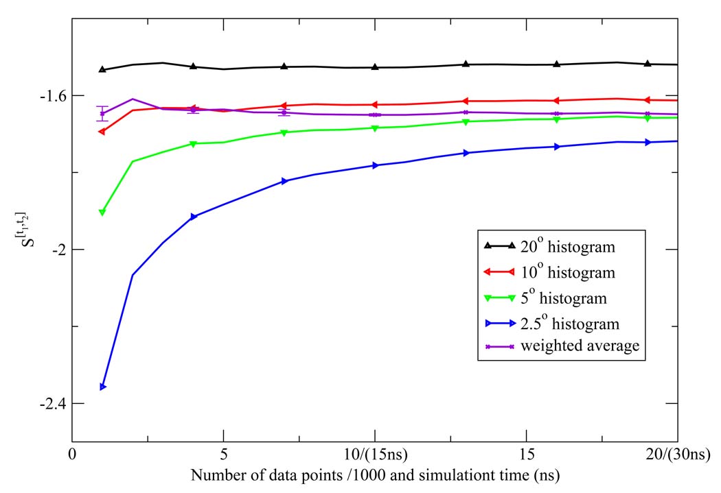
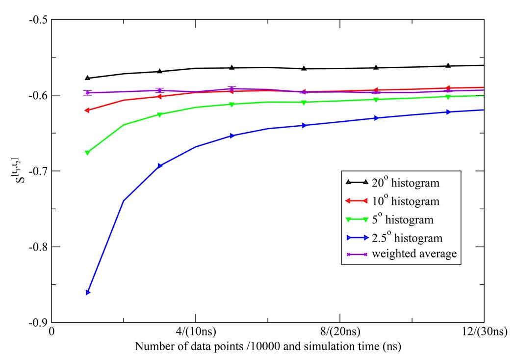
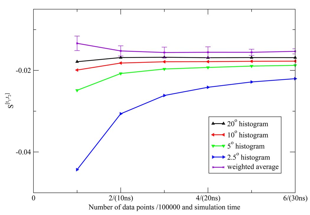
We extensively compared the commonly employed histogram method to compute the orientational Shannon entropy to the NN method weighted average (Figure 4, Figure 5, and Figure 6). We see clearly that the NN method weighted average converges much faster than histogram method for shells 1 and 2. For shell 3, both methods give similar results. This is easily understood: for the first and second shells, the water molecules are highly correlated, and the histogram results will have a strong dependency on the bin size used to do the integration; however, for the third shell, there is little correlation, so the histogram method has similar convergence properties compared to the NN method.

Figure 4.

The first shell orientational Shannon entropy S^[t₁,t₂] for the TIP3P model as a function of the number of data points (labeled on the horizontal axis in front of "/" in units of 1000) and the corresponding simulation time (labeled on the horizontal axis in parentheses) using histogram method. The weighted average of the NN estimates and the associated error bar were also depicted.

Figure 5.

The second shell orientational Shannon entropy S^[t₁,t₂] for the TIP3P model as a function of the number of data points (labeled on the horizontal axis in front of "/" in units of 10000) and the corresponding simulation time (labeled on the horizontal axis in parentheses) using histogram method. The weighted average of the NN estimates and the associated error bar were also depicted.

Figure 6.

The third shell orientational Shannon entropy S^[t₁,t₂] for the TIP3P model as a function of the number of data points (labeled on the horizontal axis in front of "/" in units of 100000) and the corresponding simulation time (labeled on the horizontal axis in parentheses) using histogram method. The weighted average of the NN estimates and the associated error bar were also depicted.

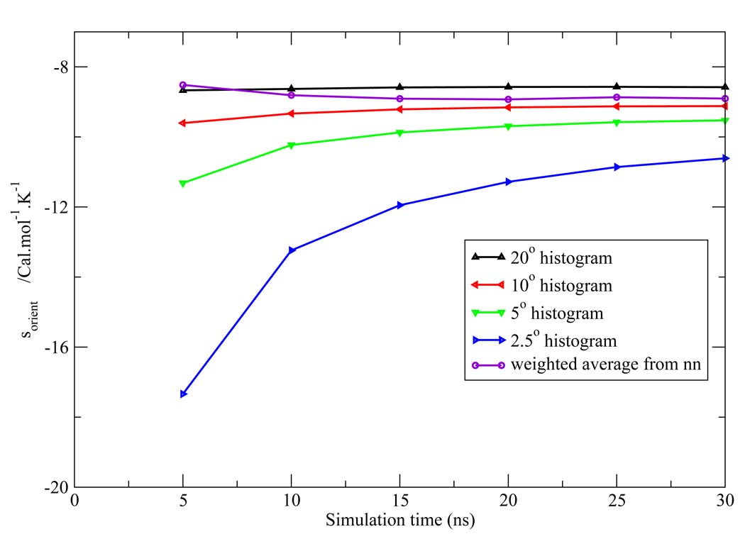
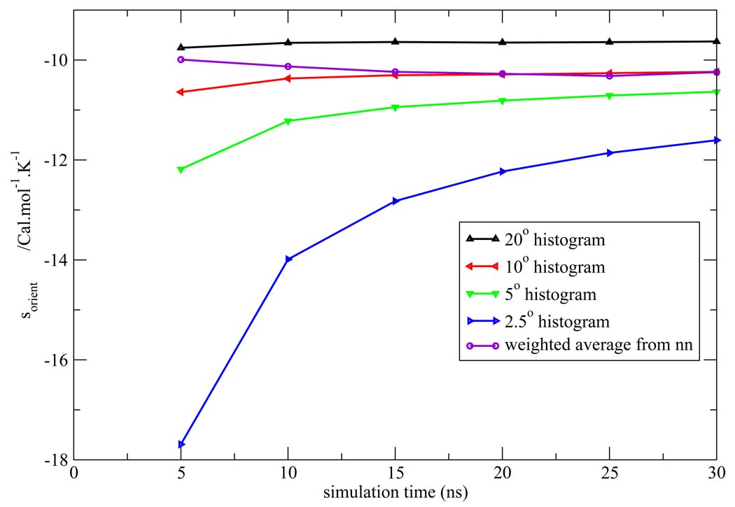
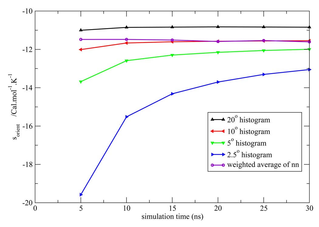
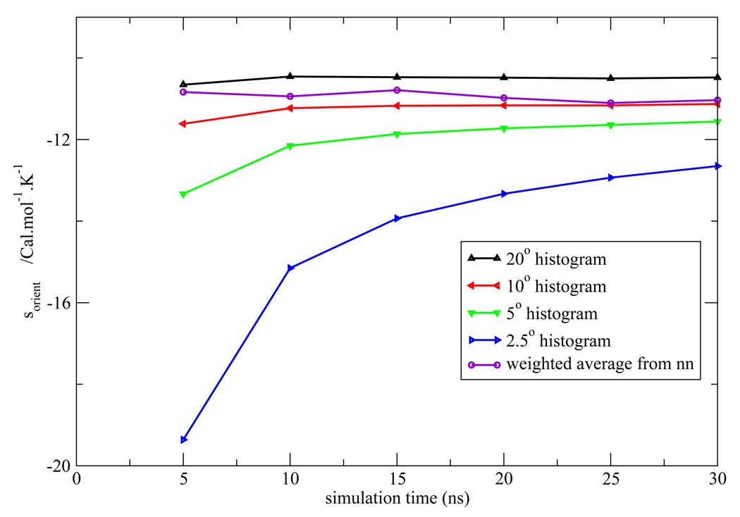
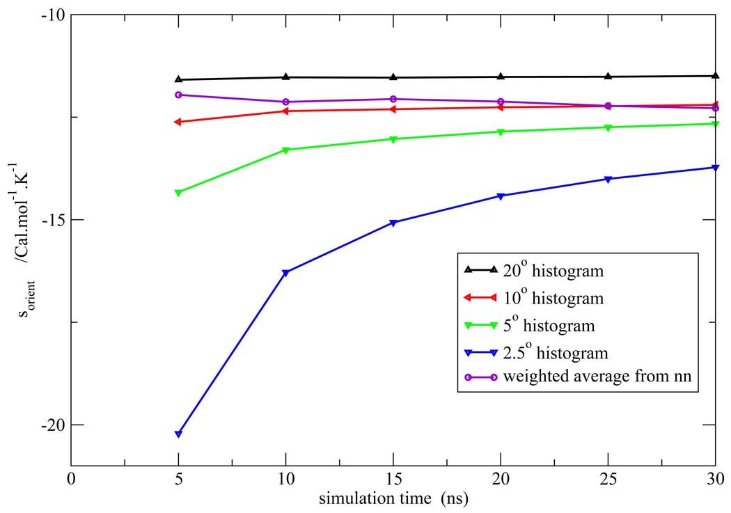
Figure 7, Figure 8, Figure 9, Figure 10, Figure 11 depict the total orientational excess entropies as a function of simulation time from the various histogram estimates and the NN weighted average estimate. For all the models studied, the 10° histogram estimate (which is most commonly used currently^6,10) gave results closest to the NN estimate. However, for a bin size of 20°, the entropy result is biased away from the correct result, and for bin sizes of 5° and 2.5°, much longer simulation time would be needed to converge the results. Since ideal bin size is problem specific, it cannot be deduced unless other reference data is already known. Thus, the absence of such a parametric bias in the NN method is a notable advantage of the technique.

Figure 7.

Total orientational excess entropy as a function of simulation time from the NN method and histogram method with different bin width for the TIP3P model.

Figure 8.

Total orientational excess entropy as a function of simulation time from the NN method and histogram method with different bin width for the SPC model.

Figure 9.

Total orientational excess entropy as a function of simulation time from the NN method and histogram method with different bin width for the SPC/E model.

Figure 10.

Total orientational excess entropy as a function of simulation time from the NN method and histogram method with different bin width for the TIP4P model.

Figure 11.

Total orientational excess entropy as a function of simulation time from the NN method and histogram method with different bin width for the TIP4P-Ew model.

3.3 Error analysis

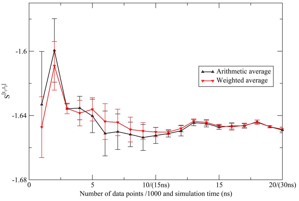
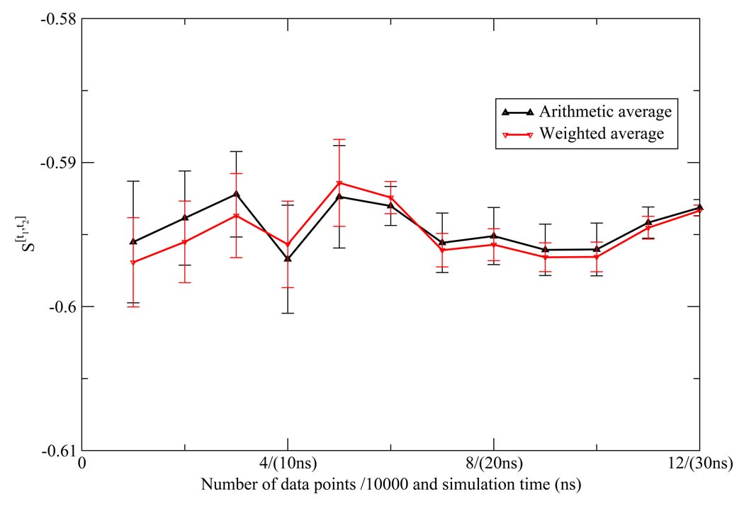
As described in the methods section, we calculated the variance associated with the weighted average of the NN estimates for each of the one and two dimensional Shannon entropies. Since the NN estimate is asymptotically unbiased, the error of the estimate is also given by the variance. We calculated the error based on the weighted average, which assumes Var ln f(x) is 0. However, even in the extreme cases where Var ln f(x) goes to infinity and the five NN estimates contribute equally to the average, the variance of the arithmetic average only differs slightly from weighted average, and they are within the error bar of each other, strongly indicating the convergence of these calculations (Figure 12 and Figure 13).

Figure 12.

Comparison between the arithmetic average and the weighted average of the NN estimates for the first shell Shannon entropy S^[t₁,t₂] for the TIP3P model. They are within the error bar of each other.

Figure 13.

Comparison between the arithmetic average and the weighted average of the NN estimates for the second shell Shannon entropy S^[t₁,t₂] for the TIP3P model. They are within the error bar of each other.

3.4 The radial dependence of orientational Shannon entropy

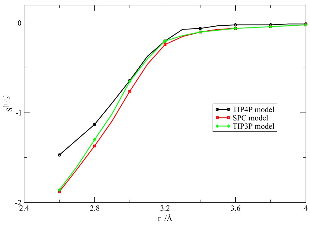
We calculated the orientational Shannon entropies in three radial regions, assuming the orientational distribution would be independent of r in each sub-region. To validate this approximation, we calculated the orientational Shannon entropies at different intervals of r from 2.5 to 4.0 Å. Typical Shannon entropies S^[t₁,t₂] at different value of r are shown in Figure 14.

Figure 14.

Orientiational Shannon entropy S^[t₁,t₂] as a function of r for the various water models.

We see from the figure that the Shannon entropy increases as the distance between the two water molecules r increases, and goes to zero when r is sufficiently large. Additionally, the change of the Shannon entropy with respect to r is smooth in the respective first and second hydration shells. Because of the slow variation of the orientational Shannon entropy with respect to r, the sum of the orientational excess entropy at each interval will differ from the sum of the orientational excess entropy of the three shells only by at most 0.5e.u., which is within statistical uncertainty of the calculation. Thus, this approximation was not a large source of error in these calculations.

3.5 Inclusion of g(θ₁,χ₁) in the factorization

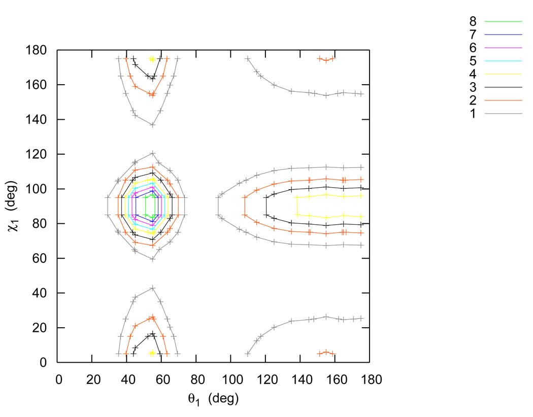
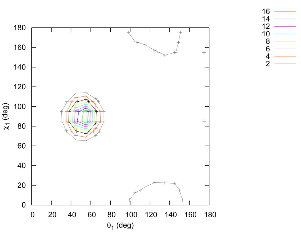
The factorization of the PCF used here differs from the more common formulation⁶ by the explicit inclusion of g(θ₁,χ₁) and g(θ₂,χ₂). The distribution functions g(θ₁) * g(χ₁) and g(θ₁,χ₁) for the TIP4P model are shown on Figure 15 and Figure 16. Careful inspection of these figures suggests that g(θ₁,χ₁) differs from g(θ₁)g(χ₁) quantitatively, which is supported by the two dimensional Shannon entropy S^{[θ₁,χ₁]} differing significantly from the sum of S^[θ₁] and S^[χ₁]. For example, for the TIP4P model the first shell Shannon entropy of S^{[θ₁,χ₁]} is −1.21, while S^[θ₁] is −0.34 and S^[χ₁] is −0.29. This result indicated a non-negligible correlation between χ₁ and θ₁, which suggested that the explicit inclusion of g(θ₁,χ₁) and g(θ₂,χ₂) in our factorization would lead to greater quantitative precision. This also explains why our excess entropy result for the TIP4P model (−13.67e.u.) is about 1.5e.u. more negative than the previously reported value (−12.2e.u.),⁶ which is in better agreement with both the FD estimate of the entropy of the model and the experimental estimate of liquid water.

Figure 15.

Products of one dimensional marginal distribution function g(θ₁) * g(χ₁) for the TIP4P model in the first shell.

Figure 16.

Two dimensional marginal distribution function g(θ₁, χ₁) for the TIP4P model in the first shell.

3.6 Comparison of free energy results

From these simulations, we computed the excess molar energies and excess free energies of the various water models. The results of these calculations for all models studied are listed in table Table 3 along side the relevant literature values. The excess free energies we have obtained here show excellent agreement (within 0.5 kcal/mol uniformly) with the high precision FEP results obtained by Shirts et. al.⁴³ Interestingly, the TIP4P model gives results closest to the experimental quantities.

Table 3.

Results for the energy, enthalpy, and entropy of liquid water from various methods

water models	TIP4P	TIP3P	SPC	SPC/E	TIP4P-Ew
excess energy	−9.85	−9.49	−9.90	−11.08	−10.91
excess enthalpy	−10.43	−10.07	−10.48	−11.66(−10.48a)	−11.49(−10.45b)
excess enthalpy*	−10.41	−10.09	−10.47	−11.69(−10.51a)	−11.61(−10.57b)
excess entropy from NN	−13.67	−11.57	−13.19	−14.72	−15.09
excess entropy**	−14.43	−13.39	−14.46	−15.57	−15.53
excess free energy from NN	−6.36	−6.63	−6.55	−7.27(−6.09a)	−7.00(−5.96b)
excess free energy*	−6.11	−6.10	−6.16	−7.05(−5.87a)	−6.98(−5.94b)
excess free energy from exp	−6.33
excess enthalpy from exp	−10.52

Energies in kcal/mol, entropies in cal/mol K (e.u.)

^*results from Shirts⁴³

^**results from Shirts⁴³ by extracting enthalpy from free energy

^aInclude polarization correction³⁹

^bInclude polarization correction⁴⁰

The SPC/E, TIP4P, and TIP4P-Ew models all give free energy results somewhat closer to the Shirts⁴³ results than the other models. This may not be accidental. In our calculations, the higher order multi-particle correlation entropies were ignored. There is some literature precedence expecting these higher order contributions to the excess entropy to vanish at the temperature of solid-liquid phase transition.^44,45 Recently, Saija has shown that for the TIP4P model, the temperature of maximum density (TMD) coincides with the temperature where higher order contributions to the entropy should vanish.¹³ Studies of temperature dependence of the densities of the different water models studied here⁴⁶ have shown that the TMD of the TIP4P model occurred at 258K, the TMD of the SCP/E model occurred at 235K,⁴⁷ the TMD of the TIP4P-Ew model occurred at 272K,⁴⁰ and the density of the SPC and TIP3P models increases monotonically as temperature decreases in the range [220,370].⁴⁶ This indicates, for the TIP3P and SPC models, multi-particle correlation entropy may contribute more to the total entropy than for the other models, which may be why our quantitative accuracy for them is somewhat diminished. However, the molecular detail afforded by this technique in yielding both a value of the entropy and a physical interpretation of its meaning, in terms of the fluid structure implied by the shape of the PCF, gives it a comparative advantage over techniques such as FEP, which will generally only yield a value of the entropy without any additional molecular understanding of the system.

3.7 Entropy calculation from FD method

We calculated the excess free energy of water at temperature 298 ± 20K with the Bennett acceptance ratio³⁰ method, and obtained entropies at 298K by the FD formula. The results are presented in Table 4. The excess entropies computed from the FD method are consistently larger in magnitude than those computed from the NN method, consistent with us neglecting the contributions from the higher order terms of the expansion.

Table 4.

Entropy results from FD method and comparison with other methods

water models	TIP4P	TIP3P	SPC	SPC/E	TIP4P-Ew
excess free energy at 278K	−6.35**	−6.21(−6.24a)	−6.36(−6.39a)	−7.19(−7.23a)	–
excess free energy at 298K	−6.03**	−5.95	–6.06	−6.89	–
excess free energy at 318K	−5.73**	−5.71(−5.69a)	−5.80(−5.78a)	−6.66(−6.62a)	–
excess entropy from FD	−15.2**	−13.8(±0.8b)	−15.2(±0.8b)	−15.3(±0.8b)	–
excess entropy from NN	−13.67	−11.57	−13.19	−14.72	−15.09
excess entropy from FEP*	−14.43	−13.39	−14.46	−15.57	−15.53

Energies in kcal/mol, entropies in cal/mol K (e.u.)

^**results from Franz Saija¹³

^*results from Shirts⁴³ by extracting enthalpy from free energy

^aresults in parentheses includes constant pressure correction(appendix B)

^bindicates the error associated with the entropy

As in the proceeding section, the NN and FD excess entropies of the SPC/E water are in very close agreement; however, the agreement of the NN and FD entropies of the SPC and TIP3P models is much poorer. We again expect the reason for this discrepancy to be due to the TMD of the SPC/E model being close to the range of temperatures treated in this study, while the TMDs of the SPC and TIP3P models fall well outside this range. Thus, the higher order terms of the entropy expansion are expected to make larger contributions to the excess entropies for the SPC and TIP3P models versus the contribution made to the excess entropy of the SPC/E water.

4 Conclusion

Our results indicate that the NN method of computing entropies in the liquid state offers several compelling advantages over the more common histogram approaches, including (1) much faster convergence for a given amount of simulation data; (2) an intuitive error bound for the uncertainty of the calculation without resorting to block averaging or bootstrapping techniques, which may be problematic to apply to estimators of the entropy; and (3) not relying on empirically tuned parameters, such as the histogram bin width, which may bias the results in an unpredictable fashion. We also found that inspection of the limiting behaviours of Var ln f(x) may be used to both analyze the convergence of the given calculation, and develop the best possible estimate of the entropy given a set of calculated H_k(n). Although we also found that a judicious choice of the histogram bin width may mitigate these advantages, such a choice is difficult to make without prior knowledge of the properties of the limiting distribution, which may not be available when new problems are investigated.

Our alternative factorization of the water-water correlation function, which explicitly included correlations between the angle formed by the water dipole vector and the intermolecular axis with the angle of rotation of the water molecule about its dipole vector, was found to increase the agreement of results obtained by the entropy expansion with those obtained by less approximate methods, such as FEP and the FD benchmark calculations. This result suggests that this contribution should not be ignored in future studies of the excess entropy of liquid water and other fluids.

Appendices

A Determination of most proper weights

Given that x₁,x₂,⋯,x_n are independent variables with the same average u but different variance v₁,v₂,⋯,v_n, we may define $\overline{x}={\displaystyle {\sum }_{i=1}^n{w}_i{x}_i}$, with constraint ${\displaystyle {\sum }_{i=1}^n{w}_i=1}$. We may find the weights w_i such that the variance of x̄ is minimized:

$$\mathit{\text{Var}}[\overline{x}]={\displaystyle \sum _{i=1}^n{(w_i)}^2{v}_i}$$ (1)

Using Lagrange multipliers we find:

$$w_i=\frac{\frac{1}{v_i}}{{\displaystyle {\sum }_{i=1}^n\frac{1}{v_i}}}$$ (2)

and

$$\mathit{\text{Var}}[\overline{x}]=\frac{1}{{\displaystyle {\sum }_{i=1}^n\frac{1}{v_i}}}$$ (3)

$$E[{\displaystyle \sum _{i=1}^n{w}_i{(x_i-\overline{x})}^2}]=E[{\displaystyle \sum _{i=1}^n{w}_i{((x_i-u)-(\overline{x}-u))}^2}]$$ (4)

$$=E[{\displaystyle \sum _{i=1}^n{w}_i({(x_i-u)}^2-2(x_1-u)(\overline{x}-u)+{(\overline{x}-u)}^2})]$$ (5)

$$\begin{array}{c}=E[{\displaystyle \sum _{i=1}^n{w}_i{(x_i-u)}^2}]-2E[{\displaystyle \sum _{i=1}^n{w}_i(x_i-u)(\overline{x}-u)}]\hfill \\ +E[{\displaystyle \sum _{i=1}^n{w}_i{(\overline{x}-u)}^2}]\hfill \end{array}$$ (6)

By application of equation 2 and ${\displaystyle {\sum }_{i=1}^n{w}_i=1}$, we find:

$$E[{\displaystyle \sum _{i=1}^n{w}_i{(x_i-\overline{x})}^2}]=\frac{n-1}{{\displaystyle {\sum }_{i=1}^n\frac{1}{v_i}}}$$ (7)

Thus we can approximate the variance of the weighted average by the estimator:

$$V=\frac{1}{n-1}{\displaystyle \sum _{i=1}^n{w}_i{(x_i-\overline{x})}^2}$$ (8)

B Constant pressure correction to ΔG_sim for the FD entropy

In the FEP simulations, we turned on/off the interaction between one distinguished water molecule with the rest of the system at constant temperature T and constant pressure P₀, over the series of several λ windows. The solvation free energy of the distinguished water molecule corresponds to the difference in the chemical potential μ between two phases: (1) the liquid phase, and (2) the ideal gas phase with the same temperature and number density as the liquid.⁴⁸ Ergo,

$$\mathrm{\Delta }{G}_{\mathit{\text{sim}}}(T)=-kT\text{ln}\frac{\tilde{\mathrm{\Delta }}(\lambda =1)}{\tilde{\mathrm{\Delta }}(\lambda =0)}={\mu }_l(N,P_0,T)-{\mu }_g(N,P^{*},T)$$ (9)

where P^* is the pressure of the ideal gas with the same temperature T and number density as the simulated liquid at pressure P₀, and Δ̃ is the isobaric-isothermal partition function of the system specified by lambda. (For details, please see reference.⁴⁸)

The heat capacity of the ideal gas at constant pressure P^* is trivially constant with respect to temperature, and we may well approximate the heat capacity of liquid water to also be constant under constant pressure P₀ over the temperature range studied here. Then it follows

$$\mathrm{\Delta }G(T)=\mathrm{\Delta }H(T)-T\mathrm{\Delta }S(T)$$ (10)

$$\mathrm{\Delta }H(T\pm \mathrm{\Delta }T)=\mathrm{\Delta }H(T)\pm \mathrm{\Delta }{C}_P\mathrm{\Delta }T$$ (11)

$$\mathrm{\Delta }S(T\pm \mathrm{\Delta }T)=\mathrm{\Delta }S(T)+\mathrm{\Delta }{C}_P\text{ln}\frac{T\pm \mathrm{\Delta }T}{T}$$ (12)

$$\mathrm{\Delta }S(T)\approx -\frac{\mathrm{\Delta }G(T+\mathrm{\Delta }T)-\mathrm{\Delta }G(T-\mathrm{\Delta }T)}{2\mathrm{\Delta }T}$$ (13)

which are the typical equations of the finite difference method of computing the thermodynamic entropy. In these equations, all the Δ quantities correspond to the difference of the thermodynamic quantities between the liquid phase at P₀ and the ideal gas phase at P^*.

In similar simulations run at pressure P₀ but temperatures T ± ΔT we analogously find

$$\mathrm{\Delta }{G}_{\mathit{\text{sim}}}(T-\mathrm{\Delta }T)={\mu }_l(N,P_0,T-\mathrm{\Delta }T)-{\mu }_g(N,P_1,T-\mathrm{\Delta }T)$$ (14)

$$\mathrm{\Delta }{G}_{\mathit{\text{sim}}}(T+\mathrm{\Delta }T)={\mu }_l(N,P_0,T+\mathrm{\Delta }T)-{\mu }_g(N,P_2,T+\mathrm{\Delta }T)$$ (15)

where P₁ and P₂ correspond to the ideal gas pressure with the same temperature and number density as the simulated liquids. Note that the ΔG values obtained from simulation differ from those occurring in equation 13 because the reference gas phase free energies differ, and thus we must explicitly correct for this difference in reference state. By adding a correction term ΔG_corr(T ± ΔT) to the simulated free energy, we were able to use equation 13 to calculate the entropy at temperature T, where:

$$\begin{array}{cc}\hfill \mathrm{\Delta }{G}_{\mathit{\text{corr}}}(T-\mathrm{\Delta }T)\hfill & ={\mu }_g(N,P_1,T-\mathrm{\Delta }T)-{\mu }_g(N,P^{*},T-\mathrm{\Delta }T)\\ & =k(T-\mathrm{\Delta }T)\text{ln}\frac{P_1}{P^{*}}\hfill \end{array}$$ (16)

$$\begin{array}{cc}\mathrm{\Delta }{G}_{\mathit{\text{corr}}}(T+\mathrm{\Delta }T)& ={\mu }_g(N,P_2,T+\mathrm{\Delta }T)-{\mu }_g(N,P^{*},T+\mathrm{\Delta }T)\\ & =k(T+\mathrm{\Delta }T)\text{ln}\frac{P_2}{P^{*}}\hfill \end{array}$$ (17)

and

$$\mathrm{\Delta }S(T)=-\frac{\mathrm{\Delta }{G}_{\mathit{\text{sim}}}(T+\mathrm{\Delta }T)+\mathrm{\Delta }{G}_{\mathit{\text{corr}}}(T+\mathrm{\Delta }T)-\mathrm{\Delta }{G}_{\mathit{\text{sim}}}(T-\mathrm{\Delta }T)-\mathrm{\Delta }{G}_{\mathit{\text{corr}}}(T-\mathrm{\Delta }T)}{2\mathrm{\Delta }T}$$ (18)

These corrections, although small in magnitude, were systematically of opposite sign at temperatures T ± ΔT because the thermal expansion coefficient of liquid water differs from the thermal expansion coefficient of the ideal gas. As a result, failure to apply these corrections will lead to a non-negligible systematical bias in the FD-FEP entropy.

The thermodynamic cycle indicating the whole process, including correction terms, is depicted in Figure 17. Note that in the cycle depicted in Figure 17, we must compute the correction terms at temperatures T ± ΔT in order to compute the slope of ΔG with respect to T, ie the entropy associated with the solvation free energy of transfering the water molecule from the gas phase to the liquid phase at temperature T.

Figure 17.

Thermodynamic cycle depicting the constant pressure corrections to ΔG_sim at temperatures T ± ΔT when computing the slope of ΔG_sim with respect to T.

References

- 1.Berne BJ, Weeks JD, Zhou R. Annu. Rev. Phys. Chem. 2009;60:85–103. doi: 10.1146/annurev.physchem.58.032806.104445. [DOI] [PMC free article] [PubMed] [Google Scholar]
- 2.Abel R, Young T, Farid R, Berne BJ, Friesner RA. J. Am. Chem. Soc. 2008;130:2817–2831. doi: 10.1021/ja0771033. [DOI] [PMC free article] [PubMed] [Google Scholar]
- 3.Young T, Abel R, Kim B, Berne BJ, Friesner RA. Proc. Nat. Acad. Sci. 2007;104:808–813. doi: 10.1073/pnas.0610202104. [DOI] [PMC free article] [PubMed] [Google Scholar]
- 4.Lazaridis T. J. Phys. Chem. B. 1998;102:3531–3541. [Google Scholar]
- 5.Lazaridis T, Paulattis ME. J. Phys. Chem. 1992;96:3847–3855. [Google Scholar]
- 6.Lazaridis T, Karplus M. J. Chem. Phys. 1996;105:4294–4316. [Google Scholar]
- 7.Li Z, Lazaridis T. J. Phys. Chem. B. 2006;110:1464–1475. doi: 10.1021/jp056020a. [DOI] [PubMed] [Google Scholar]
- 8.Li Z, Lazaridis T. J. Phys. Chem. B. 2005;109:662–670. doi: 10.1021/jp0477912. [DOI] [PubMed] [Google Scholar]
- 9.Zielkiewicz J. J. Phys. Chem. B. 2008;112:7810–7815. doi: 10.1021/jp7103837. [DOI] [PubMed] [Google Scholar]
- 10.Zielkiewicz J. J. Chem. Phys. 2005;123:104501. doi: 10.1063/1.2018637. [DOI] [PubMed] [Google Scholar]
- 11.Esposito R, Saija F, Saitta AM, Giaquinta PV. Phys. Rev. E. 2006;73:040502. doi: 10.1103/PhysRevE.73.040502. [DOI] [PubMed] [Google Scholar]
- 12.Silverstein KAT, Dill KA, Haymet ADJ. J. Chem. Phys. 2001;114:6303–6314. [Google Scholar]
- 13.Saija F, Saitta AM, Giaquinta PV. J. Chem. Phys. 2003;119:3587–3589. [Google Scholar]
- 14.Singh H, Misra N, Hnizdo V, Fedorowicz A, Demchuk E. Am. J. Math. Manag. Sci. 2003;23:301–322. [Google Scholar]
- 15.Green HS. Molecular theory of fluids. North-Holland: Amsterdam; 1952. Chapter III. [Google Scholar]
- 16.Raveché HJ. J. Chem. Phys. 1971;55:2242–2250. [Google Scholar]
- 17.Wallace DC. J. Chem. Phys. 1987;87:2282–2284. [Google Scholar]
- 18.Shannon CE. Bell. Syst. Tech. J. 1948;27:379–423. [Google Scholar]
- 19.Fisher IZ, Kopeliovich BL. Dokl. Akad. Nauk SSSR [Sov. Phys. Dokl. 5, 761 (1960)] 1960;133:81–83. [Google Scholar]
- 20.Reiss H. J. Stat. Phys. 1972;6:39–47. [Google Scholar]
- 21.Singer A. J. Chem. Phys. 2004;121:3657–3666. doi: 10.1063/1.1776552. [DOI] [PubMed] [Google Scholar]
- 22.Killian BJ, Kravitz JY, Gilson MK. J. Chem. Phys. 2007;127:024107. doi: 10.1063/1.2746329. [DOI] [PMC free article] [PubMed] [Google Scholar]
- 23.Hnizdo V, Darian E, Fedorowicz A, Demchuk E, Li S, Singh H. J. Comput. Chem. 2007;28:655–668. doi: 10.1002/jcc.20589. [DOI] [PubMed] [Google Scholar]
- 24.Matsuda H. Phys. Rev. E. 2000;62:3096–3102. doi: 10.1103/physreve.62.3096. [DOI] [PubMed] [Google Scholar]
- 25.Loftsgaarden DO, Quesenberry CP. Ann. Math. Statist. 1965;36:1049–1051. [Google Scholar]
- 26.Arya S, Mount DM. Approximate nearest neighbor queries in fixed dimensions. SODA ’93: Proceedings of the fourth annual ACM-SIAM Symposium on Discrete algorithms; Philadelphia, PA, USA. 1993. pp. 271–280. [Google Scholar]
- 27.Freidman JH, Bentley JL, Finkel RA. ACM Trans. Math. Softw. 1977;3:209–226. [Google Scholar]
- 28.Smith DE, Haymet AD. J. Chem. Phys. 1993;98:6445–6454. [Google Scholar]
- 29.Wan SZ, Stote RH, Karplus M. J. Chem. Phys. 2004;121:9539–9548. doi: 10.1063/1.1789935. [DOI] [PubMed] [Google Scholar]
- 30.Bennett CH. J. Comput. Phys. 1976;22:245–268. [Google Scholar]
- 31.Bowers KJ, Chow E, Xu H, Dror RO, Eastwood MP, Gregersen BA, Klepeis JL, Kolossvary I, Moraes MA, Sacerdoti FD. Scalable algorithms for molecular dynamics simulations on commodity clusters. In: Salmon JK, Shan Y, Shaw DE, editors. SC ’06: Proceedings of the 2006 ACM/IEEE conference on Supercomputing; New York, NY, USA. 2006. p. 84. [Google Scholar]
- 32.Jorgensen WL, Chandrasekhar J, Madura JD, Impey RW, Klein ML. J. Chem. Phys. 1983;79:926–935. [Google Scholar]
- 33.Nosé S. J. Chem. Phys. 1984;81:511–519. [Google Scholar]
- 34.Hoover WG. Phys. Rev. A. 1985;31:1695–1697. doi: 10.1103/physreva.31.1695. [DOI] [PubMed] [Google Scholar]
- 35.Martyna GJ, Tobias DJ, Klein ML. J. Chem. Phys. 1994;101:4177–4189. [Google Scholar]
- 36.Tuckerman M, Berne BJ, Martyna GJ. J. Chem. Phys. 1992;97:1990–2001. [Google Scholar]
- 37.Darden T, York D, Pedersen L. J. Chem. Phys. 1993;98:10089–10092. [Google Scholar]
- 38.Berendsen HJC, Postma JPM, van Gunsteren WF, Hermans J. Interaction Models for Water in Relation to Protein Hydration. In: Pullman B, editor. Intermolecular Forces. Reidel: Dordrecht; 1981. pp. 331–342. [Google Scholar]
- 39.Berendsen HJC, Grigera JR, Straatsma TP. J. Phys. Chem. 1987;91:6269–6271. [Google Scholar]
- 40.Horn HW, Swope WC, Pitera JW, Madura JD, Dick TJ, Hura GL, Head-Gordon T. J. Chem. Phys. 2004;120:9665–9678. doi: 10.1063/1.1683075. [DOI] [PubMed] [Google Scholar]
- 41.Henchman RH. J. Chem. Phys. 2007;126:064504. doi: 10.1063/1.2434964. [DOI] [PubMed] [Google Scholar]
- 42.Wagner W, Pruβ A. J. Phys. Chem. Ref. Data. 2002;31:387–478. [Google Scholar]
- 43.Shirts MR, Pande VS. J. Chem. Phys. 2005;122:134508. doi: 10.1063/1.1877132. [DOI] [PubMed] [Google Scholar]
- 44.Wallace DC. Int. J. Quantum Chem. 1994;52:425–435. [Google Scholar]
- 45.Giaquinta PV, Giunta G. Physca A. 1992;187:145–158. [Google Scholar]
- 46.Jorgensen WL, Jenson C. J. Comput. Chem. 1998;19:1179–1186. [Google Scholar]
- 47.Baez LA, Clancy P. J. Chem. Phys. 1994;101:9837–9840. [Google Scholar]
- 48.Horn HW, Swope WC, Pitera JW. J. Chem. Phys. 2005;123:194504. doi: 10.1063/1.2085031. [DOI] [PubMed] [Google Scholar]