Can the whole be less than the sum of its parts? Pathway analysis in genome-scale metabolic networks using elementary flux patterns

Abstract

Elementary modes represent a valuable concept in the analysis of metabolic reaction networks. However, they can only be computed in medium-size systems, preventing application to genome-scale metabolic models. In consequence, the analysis is usually constrained to a specific part of the known metabolism, and the remaining system is modeled using abstractions like exchange fluxes and external species. As we show by the analysis of a model of the central metabolism of Escherichia coli that has been previously analyzed using elementary modes, the choice of these abstractions heavily impacts the pathways that are detected, and the results are biased by the knowledge of the metabolic capabilities of the network by the user. In order to circumvent these problems, we introduce the concept of elementary flux patterns, which explicitly takes into account possible steady-state fluxes through a genome-scale metabolic network when analyzing pathways through a subsystem. By being similar to elementary mode analysis, our concept now allows for the application of many elementary-mode-based tools to genome-scale metabolic networks. We present an algorithm to compute elementary flux patterns and analyze a model of the tricarboxylic acid cycle and adjacent reactions in E. coli. Thus, we detect several pathways that can be used as alternative routes to some central metabolic pathways. Finally, we give an outlook on further applications like the computation of minimal media, the development of knockout strategies, and the analysis of combined genome-scale networks.

In functional genomics and metabolic engineering, metabolic pathway analysis has proved to be a very useful methodology (Carlson et al. 2002; Schwender et al. 2004; Feist and Palsson 2008; Trinh et al. 2009). Elementary modes (Schuster et al. 2000) are a central concept in this field. An elementary mode represents a minimal set of reactions that can operate at steady state with all reactions proceeding in their appropriate direction (Schuster et al. 2000) and, hence, can be considered as a formal definition of a metabolic pathway. Elementary modes have been used in many areas of biotechnology, such as assessing network flexibility (Stelling et al. 2002), finding pathways with optimal yields for certain metabolic species (Schuster et al. 2002a; Krömer et al. 2006), finding possible targets for the engineering of metabolic networks (Klamt 2006), and analyzing the effect of such an engineering (Carlson et al. 2002; Schwender et al. 2004). Due to the growing availability of genome-scale metabolic networks (Duarte et al. 2004, 2007; Borodina and Nielsen 2005; Thiele et al. 2005; Feist et al. 2006, 2007; Jamshidi and Palsson 2007; Oh et al. 2007) and the comprehensive analysis conducted on them (for review, see Feist and Palsson 2008), it becomes desirable to apply elementary mode analysis in such networks.

However, the principal problem encountered when trying to compute elementary modes in larger metabolic networks is that their number is growing exponentially with network size (Klamt and Stelling 2002; Schuster et al. 2002b; Acuña et al. 2009). Thus, they become difficult to analyze or even impossible to enumerate because of constraints in memory or computation time. Although there have been recent efforts to port the algorithms for the computation of elementary modes to larger networks by means of parallelization (Klamt et al. 2005) or improvements of the existing algorithms (von Kamp and Schuster 2006; Terzer and Stelling 2008), none of these algorithms permits the analysis of elementary modes in genome-scale metabolic networks.

In consequence, elementary mode analysis is applied to smaller networks containing reactions of interest rather than the entire known system. The remainder of the system is modeled using abstractions like exchange fluxes and external metabolites. Exchange fluxes correspond to the production or consumption of a species by a large set of reactions of the remaining model. External species, in contrast, are considered to be buffered by reactions of the complete system. Hence, they are excluded from the steady-state condition. However, as we show in this study, there are three important drawbacks involved in the introduction of such abstractions (cf. Liebermeister et al. 2005).

First, the approach is usually biased by the modeler's knowledge of the network. For instance, glycolysis and pentose phosphate pathways are usually considered the principal routes for the supply of metabolites from glucose in the growth media to the tricarboxylic acid (TCA) cycle. Thus, the Entner–Doudoroff pathway—which represents an alternative route for the production of pyruvate in several bacteria—is often ignored even though it is of importance in some conditions (Fischer and Sauer 2003; Li et al. 2006). In consequence, some of the possible pathways of a large network through a subnetwork are not found by elementary mode analysis (Fig. 1A). Second, the aforementioned abstractions might not be able to take into account the dependencies between the production and consumption of metabolites that constitute the interface of the subnetwork to the remaining system. This can give rise to elementary modes that obey the steady-state condition within the subnetwork but are not part of any steady-state flux through the entire network (Fig. 1B,C). Third, by only focusing on a small part of the known network, the integration of a pathway through this subnetwork into a pathway on the scale of the entire system is not straightforward, and the interdependencies between the pathways of several subsystems cannot be analyzed (Fig. 1D).

Figure 1.

Examples for problems in elementary mode analysis. (A) Condensed network of glycolysis (dark reactions) and Entner–Doudoroff pathway (gray reactions). The pentose phosphate pathway has been omitted for clarity. In most analyses of glycolysis, the Entner–Doudoroff pathway is not considered. Hence, not all pathways from glucose into the TCA cycle are found, and the wrong conclusion might be drawn that only the pentose–phosphate pathway (not shown) can be used to bypass the knockout of one of the enzymes converting G6P to FDP. In vivo the knockout of the corresponding reactions is partially bypassed by a flux through the Entner–Doudoroff pathway (Fischer and Sauer 2003). (B) Modeling the Entner–Doudoroff pathway by adding an outflow of G6P and an inflow of G3P and Pyr only partially resolves the problem (thick arrows). Such an approach is often used in elementary mode analysis to avoid the consideration of some pathways in detail (e.g., the outflow of succinyl-CoA from the TCA cycle in Schuster et al. 1999, analyzed in Results). However, this can lead to fluxes like in C, which are not part of any feasible pathway when the entire network in A is considered. This is because the coupling of the influx of Pyr with the outflow reactions of G6P and the inflow reaction of G3P are neglected in B. (D) Elementary mode analysis does not allow one to analyze the dependencies between the subsystems S₁ and S₂ unless the reactions connecting them are taken into account. Thus, it is not possible to deduce that a zero flux from G6P to FDP in S₁ would imply that there cannot be a positive flux from DHAP to G3P in S₂. A list of abbreviations can be found in Supplemental material S2.

The concept of “elementary flux patterns” that we introduce in this study circumvents these problems by taking into account the possible fluxes through the entire network, when analyzing the steady-state fluxes through a subnetwork. An elementary flux pattern is defined as a set of reactions within a subsystem of a larger network that represents the basic routes of each steady-state flux of the larger network through the subnetwork. Thus, flux modes in a subsystem can be determined that are feasible in the context of the entire genome-scale system. Through their definition, elementary flux patterns allow a consistent application of concepts from elementary mode analysis to genome-scale metabolic networks without the drawbacks that arise by the definition of external species or exchange fluxes. Furthermore, each elementary flux pattern can be mapped to at least one elementary mode in the complete system, even allowing the user to analyze pathways on the genome scale.

This article is sectioned into three main parts. First, we will introduce elementary flux patterns and an algorithm to compute them. Subsequently, we apply this concept to a genome-scale metabolic network of Escherichia coli. Then we discuss our results and give an outlook on further applications of elementary flux patterns.

Methods

Next, we will formally introduce the concepts central to this study. We start by giving a short introduction to elementary mode analysis. This is followed by a definition of elementary flux patterns and the outline of an algorithm to compute them. Subsequently, we compare our method to other approaches for pathway analysis in genome-scale metabolic networks.

A metabolic network comprising n reactions and m metabolites is defined by the m × n stoichiometric matrix M. An entry M_ij of M is negative if species i is an educt of reaction j and positive if it is a product. Since elementary flux patterns are defined within a subsystem of k reactions of the entire system, we assume for simplicity that the k first columns of M (i.e., the k first reactions) constitute the subsystem.

Elementary modes

Elementary modes represent minimal sets of reactions that can operate at steady state with all reactions proceeding in thermodynamically feasible directions (Schuster et al. 2000). They are minimal in the sense that there is no subset of reactions that could also operate at steady state.

Formally, an elementary mode is a flux vector v of length n that assigns a flux to each reaction, such that

Furthermore, v has to obey the thermodynamic constraints of the reactions; that is, if reaction i is irreversible, v_i has to be non-negative. To simplify the analysis, we adopt the widely used procedure of splitting reversible reactions into forward and backward directions. Thus, the irreversibility constraint becomes

A flux mode v is called elementary if there exists no flux mode v′ that uses a proper subset of the reactions of v (Schuster et al. 2000).

Through the concept of elementarity, the set of elementary modes of a reaction network and their superposition describe all of the possible steady states of this network. That is, each steady state can be written as a non-negative linear combination of elementary modes. As mentioned above, the analysis with elementary modes can be further simplified by the introduction of external species. External species are considered to be buffered by reactions outside of the model. Thus, the steady-state condition can be relaxed by removing the rows corresponding to external species from the stoichiometric matrix M in condition 1. This describes also the major problem when defining external species. Through removing species from M, all information on the dependencies between their production and consumption by reactions of the remaining system is lost.

Elementary flux patterns

Flux patterns are defined as sets of reactions in a subsystem of k reactions of interest in a large metabolic network. They correspond to all possible routes that a steady-state flux of the entire network can take through the subsystem. To simplify the analysis, only elementary routes are considered. Hence, a flux pattern is called elementary if it cannot be derived as a combination of at least two other flux patterns. For an example of elementary flux patterns in a subsystem of the TCA cycle and some adjacent reactions, see Figure 2.

Figure 2.

Elementary flux patterns in a condensed model of the TCA cycle and adjacent reactions. (A) Model of the entire network. The TCA cycle is chosen as a subsystem (dark reactions). (B–D) Elementary flux patterns of the system are indicated by thick black arrows. The associated pathway through the entire system is indicated by thick gray arrows. The thickness of the arrows corresponds to the relative flux through each reaction. (E) Alternative pathway through the entire system using the same reactions of the flux pattern depicted in C. While the pathway in C corresponds to the glyoxylate cycle that can be used for growth on fatty acids, E corresponds to the phosphoenolpyruvate-glyoxylate cycle used as a catabolic pathway during growth on low glucose concentrations (Fischer and Sauer 2003). A list of abbreviations can be found in Supplemental material S2.

Formally, a flux pattern s is a set of indices i with 1 ≤ i ≤ k that fulfills the following conditions (please note that we assume that the first k reactions in M represent the subsystem):

Thus, a flux pattern is a set of reactions, or, more precisely, a set of reaction indices, of the subnetwork that is part of a steady-state flux v of the entire network. We require that the indices s of v are nonzero, while the remaining are zero. Given the set of elementary flux patterns S of a system, that is, a set of sets of reaction indices, we call a flux pattern s ∈ S elementary if

Thus, we call s elementary if there exists no set of flux patterns (not including s) whose union is equal to s. Please note that this definition is less restrictive than that in the concept of elementary modes, as the elementarity of a flux mode requires that the nonzero indices of one elementary mode cannot be a subset of the nonzero indices of another elementary mode. An analogous statement for flux patterns does not hold. More details on this difference are given in the next section.

In conditions 3 to 6 no statement is made about the relationship between the reactions of the subsystem. Thus, in contrast to elementary mode analysis, reactions need not interface with each other through substrates or products. In consequence, it is possible to analyze the dependencies between different subsystems like in Figure 1D without needing to add all reactions connecting both to a combined subsystem.

Furthermore, the empty set also fulfills the flux pattern condition. However, the presence of the empty flux pattern indicates only that the zero flux Oⁿ is a valid, although trivial, solution of Equations 1 and 2; hence, it is of no interest here.

Through the splitting of reversible reactions into two irreversible reactions, spurious cycles of the forward and back direction of the reversible reaction occur. If required, they can be removed in a post-processing step.

Comparison of elementary modes and elementary flux patterns

Elementary flux patterns are tightly coupled to fluxes within the entire system. As demonstrated in Supplemental material S5.2, each elementary flux pattern is part of at least one elementary mode of the complete system. Following a procedure outlined in Supplemental material S5.3, this elementary mode can be obtained. Additionally, alternative pathways can be computed by constraining some of the reactions of such an elementary mode to zero. Furthermore, by slightly adapting the constraints in the formulation of the integer linear program used for the computation of the k-shortest elementary modes (de Figueiredo et al. 2009), it is possible to enumerate all elementary modes containing a given flux pattern (data not shown). However, the latter approach requires optimizing an integer linear program with as many integer variables as reactions in the system. This procedure is computationally very demanding.

Besides their definition in subnetworks of metabolic models, the most obvious difference between elementary modes and elementary flux patterns is that the former are defined as a vector and the latter as a set of indices. An elementary mode represents a particular flux distribution in a network, in which flux proportions are considered (although it is indeterminate with respect to scaling). In contrast, a flux pattern can correspond to several flux proportions within the genome-scale system. Hence, only the binary pattern is considered. However, most of the applications of elementary modes only require the set of nonzero indices of the elementary modes (Gagneur and Klamt 2004), called the “activity set” in Nuño et al. (1997). Thus, a reduction to mere index sets does not represent an obstacle in many applications of elementary modes.

Furthermore, if the subnetwork encompasses the entire network (k = n), each elementary flux pattern corresponds to an elementary mode of the network (see Supplemental material S5.1 for a proof).

Another difference with elementary mode analysis can be found in the splitting of reversible reactions into irreversible forward and backward directions. It has been shown that, besides spurious cycles consisting of forward and backward steps and the doubling of entirely reversible elementary modes, the set of elementary modes does not change by splitting reversible reactions (Gagneur and Klamt 2004). In principle, this statement also holds for elementary flux patterns. Replacing the positivity condition in Equation 5 by a nonzero condition for reversible reactions of the subsystem would make a splitting unnecessary. However, this would introduce ambiguities since elementary flux patterns are defined as sets of reactions, that is, as binary patterns. In consequence, each reversible reaction would also be modeled as a single index, and it would not be clear which direction of a reversible reaction is used. Thus, splitting reversible reactions simplifies the analysis.

Computation of elementary flux patterns

The elementary flux patterns of a subsystem can be computed by iteratively solving a mixed-integer linear program (MILP) that returns an elementary flux pattern. By consecutively adding additional constraints, it is assured that a new elementary flux pattern is always returned. If all elementary flux patterns have been found, the MILP becomes infeasible and the iteration is stopped. For a detailed outline of the procedure, see the Appendix.

Computational complexity

Next, we want to comment on the computational complexity of the problem of finding elementary flux patterns. As outlined in Supplemental material S4, the computation time of the algorithm presented in the Appendix is polynomial in the size of the entire system and exponential in the size of the subsystem. This effort pays in that a comprehensive view on the metabolic capabilities pertaining to the subsystem (embedded in the whole system) is obtained. The runtime complexity of the computation of elementary flux patterns is similar to that of fixed-parameter algorithms (Downey and Fellows 1998), a method by which an NP-hard problem is tackled by confining the combinatorial explosion to subproblems such as in weighted cluster editing (Böcker et al. 2008). This result is of central importance since it demonstrates that the application to larger and larger systems is not the limiting factor in the computation of elementary flux patterns.

Implementation

The algorithm has been implemented as a command-line version and a graphical user interface (GUI) in Java. The GUI enables the selection of reactions for the subnetwork as well as the analysis of elementary flux patterns. Both programs accept reaction networks in the widely used Systems Biology Markup Language (Hucka et al. 2003) as well as in a proprietary, more human-readable, format. The GUI can interface with the Systems Biology Workbench (SBW) (Sauro et al. 2003). Thus, it can be called from any SBW-compliant application. This allows an easy integration into a wide variety of tools such as network design, simulation, and further analysis that are available for SBW. The linear programs and the mixed-integer linear programs are solved using the open-source Clp and Cbc solvers from the COIN-OR project (Lougee-Heimer 2003). Cbc implements a parallelized MILP solver. Hence, the multi-processor architecture of current computer systems can be fully exploited. The running time of the algorithm for a selected list of subsystems in two genome-scale metabolic networks is given in Table 1.

Table 1.

List of subsystems of two genome-scale networks for which elementary flux patterns (EFPs) have been computed

^aThe function of the subsystem as annotated in the corresponding model.

^bComputation time was measured on an Intel Core 2 Quad Q9300 machine with 4096 MB RAM running Linux Kernel 2.6.25 and Java Hotspot VM version 1.6.0. COIN-OR Cbc version 2.0 has been used to solve the mixed-integer linear programs.

Comparison to other genome-scale pathway analysis methods

Next, we want to compare the concept of elementary flux patterns to other methods that allow pathway analysis in genome-scale metabolic networks.

Flux balance analysis

Flux balance analysis (FBA) consists of the search for a flux distribution in a reaction network that optimizes a given objective function and obeys certain constraints on reaction fluxes (Varma and Palsson 1994). A variant of FBA is called flux minimization (Holzhütter 2004). FBA has been extensively used to study metabolic networks (for review, see Raman and Chandra 2009) and has seen many extensions to take into account additional information like regulatory rules (Covert et al. 2001; Shlomi et al. 2007) and reaction kinetics (Covert et al. 2008). Like elementary flux pattern analysis, FBA can be readily used to find a pathway producing a certain metabolite. However, our method is better suited for the exhaustive enumeration of pathways in a subsystem. Furthermore, FBA meets the problem that usually most of the reactions of a computed flux are used for balancing of cofactors like ATP, NADH, or NADPH, and, hence, it is not straightforward to extract the underlying pathway used for the conversion of a source species into a target species. In elementary flux pattern analysis, this does not occur unless cofactor balancing reactions are explicitly considered in the subsystem.

Furthermore, the determination of a global pathway using the reactions of a flux pattern in a subsystem uses a linear programming method similar to FBA. Thus, elementary flux pattern analysis is, in a sense, a combination of elementary mode analysis and FBA.

Flux variability analysis

Flux variability analysis extends flux balance analysis by allowing one to determine the individual minimal and maximal fluxes of reactions given that the optimal value of an objective function is maintained (Mahadevan and Schilling 2003). Thus, it is possible to identify which reactions might be used by an optimal flux. However, it is not possible to obtain a comprehensive overview on all possible pathways but only on a subset of all reactions that can be used to achieve an optimal value of the objective function (Mahadevan and Schilling 2003).

Flux coupling analysis

Flux coupling analysis (Burgard et al. 2004) extends the concept of enzyme subsets (Pfeiffer et al. 1999). It allows one to detect global dependencies in the use of reactions at steady state by determining how fluxes through pairs of reactions are coupled to each other. As outlined in Supplemental material S7, the application of flux coupling analysis can be seen as a special case of elementary flux pattern analysis in all subsystems containing only two reactions. In consequence, results from flux coupling analysis can similarly be obtained by using elementary flux pattern analysis. Our method can be seen as a generalization of flux coupling analysis since it not only examines the dependencies between pairs of reactions, but also between any subset of reactions within a subsystem.

Results

We analyzed a model of the tricarboxylic acid cycle (TCA cycle), the glyoxylate shunt, and associated reactions in E. coli that has been previously analyzed using elementary modes (Schuster et al. 1999). We started from the genome-scale metabolic model of E. coli from Feist et al. (2007) and defined the subsystem as the set of reactions that were used for the elementary mode analysis by Schuster et al. (1999). We modified the genome-scale model by adding an inflow for glucose and other basic compounds that are necessary for the production of biomass (see Supplemental material S1 for a complete list). The subsystem is depicted in Figure 3. The final network contains 1972 species and 3559 reactions.

Figure 3.

Scheme of part of the central metabolism of E. coli, which is here studied as a subnetwork of a genome-scale network. A list of abbreviations can be found in Supplemental materials S2 and S3.

In the first step, we did not incorporate into the subsystem the output fluxes used in the elementary mode analysis. Elementary mode analysis requires these fluxes to guarantee a steady-state flux corresponding to the production of a certain species. Such fluxes correspond to the assumption that a certain species can be consumed by reactions outside of the subnetwork without using any further flux through the subnetwork. Since elementary flux pattern analysis takes into account the entire network, we do not need to add such abstract reactions.

Elementary modes of the system

In a first step, we analyzed the elementary modes that have been found by Schuster et al. (1999) using the method outlined in Supplemental material S5.4. Thus, we checked for each elementary mode whether it could be part of a steady-state flux through the entire system. Ten out of the 16 elementary modes given in Schuster et al. (1999) are part of such a steady-state flux, while all six elementary modes producing the external species succinyl-CoA are not. Even though there are four reactions in the complete network consuming succinyl-CoA, all of them need additional species that can only be produced at a positive rate using intermediates of the TCA cycle. Since the TCA cycle is part of the subsystem, each elementary mode producing succinyl-CoA needs an additional flux through the subsystem in order to metabolize succinyl-CoA. This is confirmed by an overview of the reactions consuming succinyl-CoA, given in Table 2.

Table 2.

List of reactions consuming succinyl-CoA in the network of Feist et al. (2007)

A list of abbreviations can be found in Supplemental materials S2 and S3.

As an example, succinyl-CoA is consumed in lysine synthesis, in which oxaloacetate is also used. Later in that pathway, succinate is released. The subsystem model used by Schuster et al. (1999) cannot properly take into account the coupling between the fluxes of succinyl-CoA consumption, oxaloacetate consumption, and succinate regeneration on that route. Most interestingly, entry number 3 in Table 2 does not require any additional substrate besides succinyl-CoA. However, if succinyl-CoA is consumed during propionate utilization, additionally, oxaloacetate is converted into pyruvate. Oxaloacetate cannot be reconverted into pyruvate unless the reactions of the subsystem are used. Thus, even in the case of propionate utilization, the degradation of succinyl-CoA requires an additional flux through the subsystem.

Elementary flux patterns of the system

In a next step, we computed the elementary flux patterns of the subsystem. To be able to analyze the production and consumption of amino acids as it has been done by Schuster et al. (1999), the outflow reactions for the biomass forms of alanine, aspartate, and glutamate present in the genome-scale network were added to the subsystem. As mentioned above, there is no such outflow reaction for succinyl-CoA, since this species can only be further metabolized using additional fluxes from the subsystem. Additionally, we added a reaction allowing the transport of alanine from the cytosol to the periplasmic space. In the model of Feist et al. (2007), species are drained from the model only in their extracellular forms. Since the model did not contain any mechanism transporting alanine to the extracellular space, such a reaction needed to be added. This system gives rise to 83 elementary flux patterns, of which eight produce one of the amino acids. In contrast, Schuster et al. (1999) found only 16 elementary modes. This shows the arbitrariness involved in the definition of exchange reactions with the remaining system necessary for elementary mode analysis. As we will outline in the following, there are several additional intermediates of the subsystem besides 2-phosphoglycerate that can be produced from glucose. Additionally, there are several pathways bypassing some of the reactions in the subsystem. This leads to many additional pathways through the subsystem in comparison to those detected by Schuster et al. (1999).

Sometimes elementary flux patterns are cryptic when considering only the reactions of the subsystem they contain. In such a case, an analysis of the genome-scale elementary modes associated to each elementary flux pattern is necessary. This can be accompanied by constraining the fluxes of some reactions to zero to investigate alternative elementary modes to which an elementary flux pattern corresponds. One example is the reaction of malate to oxaloacetate. There are two enzymes catalyzing this reaction, malate dehydrogenase (Mdh) and malate:quinone oxidoreductase (Mqo). Since we only took into account the reactions used in Schuster et al. (1999), we added only the reaction of Mdh to the subsystem. However, elementary modes can also use Mqo not present in the subsystem. Indeed, we find many elementary flux patterns producing malate and consuming oxaloacetate without the intermediate action of Mdh.

Entry points into the TCA cycle

Even though we considered glycolysis as the principal pathway for producing TCA cycle intermediates, we found many pairs of elementary flux patterns that differ only in the routes producing these intermediates. In each such pair, one elementary flux pattern uses 2-phosphoglycerate as the entry point, while the other uses pyruvate. There are several pathways capable of producing pyruvate from glucose without the use of glycolysis. One is the Entner–Doudoroff pathway (Fig. 4B), which is used by some bacteria as an alternative pathway to glycolysis, even though it has a lower ATP yield. In E. coli, it was found that a knockout of the glycolysis enzyme phosphoglucose isomerase resulted in an up-regulation of the Entner–Doudoroff pathway when grown on glucose (Fischer and Sauer 2003). In consequence, 30% of the glucose was metabolized through the Entner–Doudoroff pathway.

Figure 4.

Alternative pathways in the central metabolism of E. coli. Dashed arrows represent condensed reactions. (A) Alternative glyoxylate producing pathway; (B) Entner–Doudoroff pathway; (C) glycerate pathway; (D) GABA-shunt. The lower pathway represents the standard route from oxoglutarate to succinate in the TCA cycle, and the upper pathway depicts the GABA shunt. A list of abbreviations can be found in Supplemental materials S2 and S3.

The principal pathway connecting glycolysis to the TCA cycle proceeds via the conversion of pyruvate to acetyl-CoA and carbon dioxide. However, the consumption of acetyl-CoA does not allow a positive production rate of any of the species of the TCA cycle (Weinman et al. 1957; Schuster and Fell 2007). Thus, TCA cycle intermediates need to be replenished using an additional inflow from, for example, glycolysis or malate from the glyoxylate bypass. In this context, we found an elementary flux pattern that is capable of producing phosphoenolpyruvate from acetyl-CoA via the glyoxylate bypass. This is an interesting case since the network is supplied with glucose as carbon source. However, a pathway different from glycolysis is used to produce acetyl-CoA from glucose. An example for such a pathway is the production of pyruvate by the Entner–Doudoroff pathway and the subsequent reaction of pyruvate and coenzyme A to formate and acetyl-CoA catalyzed by the pyruvate formate lyase. Within the subsystem, acetyl-CoA is subsequently converted into phosphoenolpyruvate using the glyoxylate shunt.

The fourth entry point necessitates the production of acetyl-CoA and glyoxylate by sources outside of the subsystem. More details about this pathway are given in the next section.

An alternative source for glyoxylate

While isocitrate lyase is used in the glyoxylate bypass to produce glyoxylate, we found several elementary flux patterns that use up glyoxylate, which is produced without isocitrate lyase present. Most interestingly whenever we encountered such a case, aspartate aminotransferase was operative. Constraining the flux of this reaction to zero prevented glyoxylate production through the alternative pathway. Aspartate aminotransferase produces aspartate and oxoglutarate from glutamate and oxaloacetate. Oxoglutarate can be aminated into glutamate, counterbalancing the consumption of glutamate by this reaction. Aspartate is essential for a reaction in the synthesis of the purine base inosine. Using several reactions, this compound is subsequently converted into glyoxylate via the intermediate of inosine-monophosphate and urate. Some central reactions of this pathway are depicted in Figure 4A.

The glycerate pathway

Some elementary flux patterns containing isocitrate lyase, the first enzyme of the glyoxylate bypass, do not contain the malate synthase catalyzing the formation of malate from glyoxylate and acetyl-CoA. These elementary flux patterns use the glycerate pathway (Hansen and Hayashi 1962) that condenses two glyoxylates to 2-hydroxy-3-oxopropanoate and produces either 2-phosphoglycerate or 3-phosphoglycerate (Fig. 4C). An interesting aspect of this pathway is that it needs only three steps to produce 3-phosphoglycerate from glyoxylate. Thus, it might be of importance during gluconeogenesis from acetyl-CoA since the common glucogenic route via malate needs five reactions for the same conversion.

The GABA shunt

In some elementary flux patterns that contain most of the reactions of the TCA cycle, the reactions from oxoglutarate to succinyl-CoA and further to succinate are missing, while oxoglutarate is produced and succinate is consumed from sources outside the subsystem. In these cases, reactions belonging to a pathway known in plants as the gamma-aminobutyric acid shunt (GABA shunt) are used. This pathway produces succinate from oxoglutarate via the intermediate of succinic semialdehyde (Fig. 4D). While GABA has been primarily considered in the context of acid resistance in E. coli (Richard and Foster 2003), a recent study suggested a role beyond stress response in plants and proposed the GABA shunt to be an integral part of the TCA cycle (Fait et al. 2008). Thus, this pathway might also be of importance as a bypass for a part of the TCA cycle in E. coli. However, its role as such a bypass has, to our knowledge, not yet been investigated in detail.

Amino-acid-producing elementary flux patterns

We found eight elementary flux patterns producing amino acids (Fig. 5). A single elementary flux pattern produces alanine (Fig. 5A), while aspartate is produced by three elementary flux patterns (Fig. 5B–D) and glutamate by four elementary flux patterns (Fig. 5E–H).

Figure 5.

Amino acid producing elementary flux patterns. (A) Alanine; (B–D) aspartate; (E–H) glutamate. Black reactions belong to the elementary flux pattern; gray reactions are the remaining reactions of the subsystem. A list of abbreviations can be found in Supplemental materials S2 and S3.

The elementary flux pattern producing alanine contains only two reactions, the production of alanine from pyruvate and glutamate as well as the outflow of extracellular alanine. Hence, the substrates of the reaction producing alanine can be replenished from sources outside the subsystem. This is corroborated by our previous finding that pyruvate, which is aminated into alanine, can be produced without using glycolysis. Furthermore, glutamate can be produced from oxoglutarate using one of several transaminase reactions not included in the subsystem.

The number of elementary flux patterns producing glutamate are due to the possible entry points of species into the subsystem. These are acetyl-CoA alone or in conjunction with either 2-phosphoglycerate, pyruvate, or glyoxylate (via the alternative glyoxylate-producing pathway). The route via glyoxylate involves the alternative pathway of glyoxylate production depicted in Figure 4A. Thus the action of the aspartate aminotransferase is also necessary.

For aspartate, only three of the entry points are used by the elementary flux patterns. Producing aspartate, using acetyl-CoA, and the glyoxylate bypass is a flux pattern, but does not fulfill the elementarity condition. An explanation is in order.

Each pathway drawing species from the TCA cycle with acetyl-CoA alone entering the cycle needs to include the glyoxylate bypass. This pathway requires the malate synthase and the fumarase to replenish oxaloacetate. Additionally, the aspartate transaminase is necessary to produce aspartate from oxaloacetate. The pathway using glyoxylate (from the alternative glyoxylate producing pathway) and acetyl-CoA as substrates also requires the malate synthase and the fumarase. As depicted in Figure 6, the fumarase is needed in order to reconvert fumarate consumed by the alternative glyoxylate-producing pathway in Figure 4A into aspartate. Any flux pattern producing aspartate using acetyl-CoA as entry point into the subsystem would be a union of two elementary flux patterns. The first is the elementary flux pattern containing the reactions of the subsystem corresponding to the alternative glyoxylate-producing pathway; and the second, the aspartate-producing elementary flux pattern in Figure 6.

Figure 6.

Elementary flux pattern belonging to an aspartate-producing pathway. (Bold arrows) The reactions of the elementary flux pattern (i.e., they belong to the subsystem). The species entering the subsystem are acetyl-CoA and glyoxylate via the alternate glyoxylate-producing pathway presented in Figure 4A. (Dashed lines) Condensed reaction. Selected fluxes are given. A list of abbreviations can be found in Supplemental materials S2 and S3.

Another interesting aspect arises from the observation that, only for glutamate, no reaction from the subsystem producing this amino acid is necessary. However, the production of oxoglutarate appears in any flux pattern producing glutamate. Thus, while the reactions of the subsystem are necessary to produce oxoglutarate, the conversion into glutamate can also be performed by reactions outside the subsystem.

Discussion

Here we have introduced elementary flux pattern analysis as a new concept for the investigation of pathways in genome-scale metabolic networks. In contrast to elementary modes, which represent an important tool for the analysis of metabolic networks, they more accurately depict the metabolic capabilities of a subsystem integrated into a genome-scale model and offer several important advantages.

First, the modeling of the interaction of the subsystem with the entire model is not biased by the knowledge of pathways into and out of the subsystem by the modeler, which might be limited to pathways seen under standard conditions. Thus, instead of 16 pathways through the TCA cycle and some adjacent reactions found with elementary mode analysis in Schuster et al. (1999), we detected 83 possible routes. We started with 2-phosphoglycerate as the principal species produced from glucose that served as input to the subsystem. However, our analysis found four possible input points, including a previously unknown pathway producing glyoxylate from glucose-6-phosphate without the intermediate action of one of the essential enzymes of the glyoxylate bypass. Moreover, we identified a pathway that is similar to the GABA shunt in plants and may serve to bypass some of the reactions in the TCA cycle.

Second, constraints imposed by the stoichiometric structure of the entire network upon possible fluxes in the subsystem are properly taken into account. In a network analyzed in Schuster et al. (1999), we found that such constraints lead to the problem that six of the 16 reported elementary modes were not part of any steady-state flux through the entire system. Generally, referring to the questions posed in the title of this article, when metabolic subsystems are combined to larger networks, usually some of the combinations of elementary modes and, thus, pathways drop out. This is because of some metabolites that were external in the subsystems and now have to fulfill the steady-state condition since they became internal. This example shows that the set of pathways in the whole metabolic network is smaller than the “sum” of the pathway sets on the local scale.

Third, the possibility to analyze the interaction between different subsystems of a metabolic network represents a promising avenue of further research in order to gain a better understanding of the intricate structure of metabolism.

Fourth, most of the tools building on elementary mode analysis only necessitate the sets of reactions of the elementary modes. Hence, these methods can also use elementary flux patterns as a base, now allowing their application to genome-scale metabolic networks. These applications include the development of gene-knockout strategies for strain improvement and the analysis of the robustness of metabolic networks, as outlined next.

In order to prove the utility of elementary flux patterns, we chose the detection of unconventional metabolic pathways in the central metabolism of E. coli as the main focus of our work. The knowledge of such pathways is not only of theoretical interest but also of importance in many fields of biotechnology, for instance, in the analysis of gene knockout experiments and metabolic flux analysis (Wittmann 2007). In the analysis of gene knockout experiments, our method can help to identify alternative pathways that might be used to bypass a knockout. In metabolic flux analysis, our method can help to improve the stoichiometric models used for the calculation of intra-cellular reaction fluxes from labeling experiments. These models usually only include a specific part of the entire metabolism. Hence, they face the same problem as elementary mode analysis, by potentially not taking into account all of the possible routes into and out of the subsystem. In consequence, refining the subsystem after studying its connection to the entire known metabolism using elementary flux patterns can help to improve the calculated fluxes. This can be of special importance if the cell is subject to extreme conditions resulting in a redirection of fluxes from pathways seen under standard conditions to alternative pathways (Fischer and Sauer 2003; Wittmann et al. 2007).

Finally, we want to outline some further applications of elementary flux patterns.

Determining minimal media

Elementary flux patterns can be used to compute the composition of minimal media, that is, the set of metabolites minimally required for the production of a desired product (Fig. 7). Note that some (but not necessarily all) elementary flux patterns correspond to minimal media (Fig. 7). This is of special interest for the determination of growth media required for the synthesis of complex metabolites like antibiotics (Tollnick et al. 2004). One focus could be the analysis of the different proposed growth media with respect to efficiency of the production of the antibiotic and the cost for the production of the metabolites used in the medium. Furthermore, if the network contains a reaction that indicates which metabolites are essential for the growth of the cell, it is possible to compute all minimal growth media.

Figure 7.

Determining minimal media for the production of amino acids. (A) Network under consideration for computation of elementary flux patterns. Dark reactions belong to the subsystem. (B) Elementary flux patterns of the subsystem. The inflow reaction that is used and the amino acid that can be produced from this input medium are indicated. Examples of minimal and nonminimal media are provided by the synthesis of histidine, which can be produced from glutamate alone as well as from ammonia and glutamate, respectively. The latter elementary flux pattern is more efficient in terms of glutamate consumed. A list of abbreviations can be found in Supplemental material S2.

Computing minimal cut sets

Minimal cut sets correspond to minimal sets of reactions that need to be removed from a system in order to suppress any steady-state flux performing a certain function (Klamt 2006). Such a function can be, for instance, the production of a side-metabolite by a target reaction in order to increase the yield of a desired product. A scenario for the application of elementary flux patterns in this context is outlined in Figure 8. Due to the size of the system in which elementary flux patterns can be computed, they now allow computing minimal cut sets even in genome-scale metabolic networks.

Figure 8.

Scenario for the application of minimal cut sets. (A) Reaction network under consideration, which is supplied with acetate and glutamate. It is assumed that the production of histidine should be prevented. Histidine is produced from the central metabolism intermediate ribose-5 phosphate (Umbarger 1978). Assuming that it is not possible to entirely knock out the reactions r₁₇ and r₁₈ that directly produce ribose-5 phosphate, the reactions r₁₀–r₁₅ are defined as alternative targets (black reactions). (B) In order to determine minimal cut sets, r₁₀–r₁₅ are added to the subsystem containing the outflow reaction of histidine. From the elementary flux patterns, the minimal cut sets can be obtained. (C) Minimal sets of reactions that need to be knocked out to suppress the production of histidine: (black crosses) MCS1; (dark gray crosses) MCS2; (light gray crosses) MCS3. Subsequently, the minimal cut sets can be ranked according to different criteria, like side effects or required effort to knock out the corresponding genes, to determine the optimal knockout strategy. A list of abbreviations can be found in Supplemental material S2.

Determining the robustness of metabolic networks

In a previous study, we used elementary modes to define a general measure for the susceptibility of reaction networks to knockouts (Behre et al. 2008). However, this approach builds on elementary modes, and, thus, the robustness is only determined for elementary modes of a subnetwork that might not reflect all the potential pathways as detected by elementary flux pattern analysis. Hence, elementary flux patterns allow for a more realistic assessment of the robustness.

Analysis of host–pathogen interactions

The cost for the computation of elementary flux patterns only scales polynomially with the size of the underlying genome-scale network. Thus, it is possible to analyze large-scale networks that are made up of several genome-scale metabolic networks. As such, it is possible, for instance, to define a subsystem that contains metabolic reactions of a host and vital reactions of a parasite in order to determine the interplay between the metabolisms of both organisms (Raghunathan et al. 2009). In this context, an interesting application is to determine which combinations of exchange reactions with the medium of the parasite in the host can be impaired in order to harm the parasite.

In summary, the concept of elementary flux patterns opens up an entire new avenue for the analysis of genome-scale metabolic networks. It allows for the incorporation of all the information available in a genome-scale metabolic network when analyzing a specific subsystem. This is of central importance, since a comprehensive knowledge about the, for instance, 3359 reactions and 1972 species in the model of the metabolism of E. coli by Feist et al. (2007) is difficult to achieve.

Appendix

As in the main text, we assume that the first k columns (i.e., reactions) of the stoichiometric matrix M correspond to the reactions of the subsystem. We will outline the algorithm for the computation of elementary flux patterns by first demonstrating how a linear program can be formulated that allows to test whether a set of reactions fulfills the flux pattern condition (conditions 3 to 6). Then we proceed by integrating this linear program into a mixed-integer linear program that allows us to enumerate all elementary flux patterns.

Each flux pattern s is part of at least one flux through the entire system that fulfills two conditions. First, v needs to balance all species—that is, it needs to be at steady state; and second, v needs to obey the irreversibility of some reactions. Since we split reversible reactions into two irreversible forward and backward steps, this is equivalent to the condition that all fluxes need to be non-negative. In terms of a linear program with the variables v, this translates into the constraints:

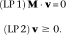Furthermore, we require that v has nonzero entries for the reactions of the flux pattern s and zero entries for the remaining reactions of the subsystem. Thus, we add

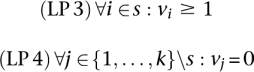as additional constraints. Note that we require that v_i ≥ 1 because it is not possible to formulate the constraint v_i > 0 in a linear program. Since the constraints do not impose any upper bounds on v, the constraint v_i > 0 is equal to v_i ≥ 1. To fulfill the flux pattern condition, we only need to test whether v exists. Thus, we only need to check the feasibility of the linear program, and no objective function is required.

In order to find all elementary flux patterns, we need to combine constraints LP 1 and LP 2 with a mixed-integer linear program. Doing this, we first need to introduce a mapping from v to a binary variable b ∈ {0, 1}^k indicating the reactions used by v in the subsystem. b_i = 1 indicates that reaction i of the subsystem is used, and b_i = 0 indicates the contrary. Thus, in addition to (LP 1) and (LP 2), we add the constraint:

with a sufficiently large constant c. If b_i = 0, the lower and upper bounds of this constraint are 0, hence v_i is constrained to zero. In the other direction, b_i = 1 implies that 1 ≤ v_i ≤ c. Hence, v_i is larger than 1 and smaller than c. In consequence, c has to be chosen either as the maximal velocity of reaction i or as a general maximal reaction velocity of the network under consideration. b indicates the reactions the flux vector v is using in the subsystem and, hence, corresponds to a flux pattern. Thus, we introduce the mapping:

from b to the encoded flux pattern. The idea of the MILP is to iteratively search for elementary flux patterns until no further flux pattern can be found. This can be achieved by iteratively solving the MILP and removing, each time, the set of previously found elementary flux patterns S from the solution space by adding an additional constraint. We can exclude previously found elementary flux patterns by requiring that each new flux pattern cannot be written as a combination of previously found elementary flux patterns. In order to implement this constraint in the MILP, we first need to reformulate it. This can be done by taking a closer look at the reactions contained in Θ(b). If we find that each reaction r ∈Θ(b) is also contained in a previously found elementary flux pattern s′ ∈S that is a subset of Θ(b), this implies that Θ(b) is a combination of elements from S. Since the contrary also holds, we need to ensure that Θ(b) contains at least one r that is not an element of any previously found elementary flux pattern that is a subset of Θ(b). This can be achieved by introducing an additional set of binary variables h ∈{0, 1}^k with h_i = 1 indicating that reaction i is an element of Θ(b) and not an element of any elementary flux pattern s′ ∈S that is a subset of Θ(b). In consequence, h_i can only equal 1 if b_i does so. Thus, we add the constraint:

Furthermore, we want for each h_i = 1 that reaction i is not an element of any s′ that is a subset of Θ(b). For each s′, we can count the number of common elements with Θ(b) by the sum . This sum is equal to the number of elements |s′| in s′ if and only if s′ is a subset of Θ(b). Thus, we add the constraint:

In consequence, if s′ is a subset of Θ(b), all h_i with i ∈s′ are constrained to zero. Conversely, each h_r = 1 indicates a reaction r that is not an element of any elementary flux pattern in S that is a subset of Θ(b). In order to ensure that we find at least one reaction r ∈Θ(b) that fulfills this condition, we add

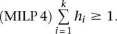Thus, we ensure that Θ(b) is not a combination of previously found elementary flux patterns. To guarantee that we find only flux patterns that are elementary, the objective function for the MILP is the minimization of , the number of reactions of the flux pattern Θ(b) [for the proof of elementarity of Θ(b), see Supplemental material S6].

In each iteration, the MILP returns a new elementary flux pattern. Finally, we obtain no further solution if all elementary flux patterns have been found. For a condensed list of the constraints of the MILP, see Supplemental material S6.

References

- Acuña V, Chierichetti F, Lacroix V, Marchetti-Spaccamela A, Sagot MF, Stougie L. Modes and cuts in metabolic networks: Complexity and algorithms. Biosystems. 2009;95:51–60. doi: 10.1016/j.biosystems.2008.06.015. [DOI] [PubMed] [Google Scholar]
- Behre J, Wilhelm T, von Kamp A, Ruppin E, Schuster S. Structural robustness of metabolic networks with respect to multiple knockouts. J Theor Biol. 2008;252:433–441. doi: 10.1016/j.jtbi.2007.09.043. [DOI] [PubMed] [Google Scholar]
- Böcker S, Briesemeister S, Bui QBA, Truß A. Proceedings of Asia-Pacific Bioinformatics Conference (APBC 2008) volume 5. Imperial College Press; London, UK: 2008. A fixed-parameter approach for weighted cluster editing; pp. 211–220. Series on Advances in Bioinformatics and Computational Biology. [Google Scholar]
- Borodina I, Nielsen J. From genomes to in silico cells via metabolic networks. Curr Opin Biotechnol. 2005;16:350–355. doi: 10.1016/j.copbio.2005.04.008. [DOI] [PubMed] [Google Scholar]
- Burgard AP, Nikolaev EV, Schilling CH, Maranas CD. Flux coupling analysis of genome-scale metabolic network reconstructions. Genome Res. 2004;14:301–312. doi: 10.1101/gr.1926504. [DOI] [PMC free article] [PubMed] [Google Scholar]
- Carlson R, Fell D, Srienc F. Metabolic pathway analysis of a recombinant yeast for rational strain development. Biotechnol Bioeng. 2002;79:121–134. doi: 10.1002/bit.10305. [DOI] [PubMed] [Google Scholar]
- Covert MW, Schilling CH, Palsson BØ. Regulation of gene expression in flux balance models of metabolism. J Theor Biol. 2001;213:73–88. doi: 10.1006/jtbi.2001.2405. [DOI] [PubMed] [Google Scholar]
- Covert MW, Xiao N, Chen TJ, Karr JR. Integrating metabolic, transcriptional regulatory and signal transduction models in Escherichia coli. Bioinformatics. 2008;24:2044–2050. doi: 10.1093/bioinformatics/btn352. [DOI] [PMC free article] [PubMed] [Google Scholar]
- de Figueiredo LF, Podhorski A, Rubio A, Beasley JE, Schuster S, Planes FJ.Troch I, Breitenecker F, editors. Calculating the k-shortest elementary flux modes in metabolic networks. Proceedings MATHMOD 09 Vienna—full papers CD volume. 2009. pp. 736–747. http://www.mathmod.at/index.php?id=115.
- Downey RG, Fellows MR. Monographs in computer science. Springer; New York: 1998. Parameterized complexity; pp. 489–516. [Google Scholar]
- Duarte NC, Herrgård MJ, Palsson BØ. Reconstruction and validation of Saccharomyces cerevisiae iND750, a fully compartmentalized genome-scale metabolic model. Genome Res. 2004;14:1298–1309. doi: 10.1101/gr.2250904. [DOI] [PMC free article] [PubMed] [Google Scholar]
- Duarte NC, Becker SA, Jamshidi N, Thiele I, Mo ML, Vo TD, Srivas R, Palsson BØ. Global reconstruction of the human metabolic network based on genomic and bibliomic data. Proc Natl Acad Sci. 2007;104:1777–1782. doi: 10.1073/pnas.0610772104. [DOI] [PMC free article] [PubMed] [Google Scholar]
- Fait A, Fromm H, Walter D, Galili G, Fernie AR. Highway or byway: The metabolic role of the GABA shunt in plants. Trends Plant Sci. 2008;13:14–19. doi: 10.1016/j.tplants.2007.10.005. [DOI] [PubMed] [Google Scholar]
- Feist AM, Palsson BØ. The growing scope of applications of genome-scale metabolic reconstructions using Escherichia coli. Nat Biotechnol. 2008;26:659–667. doi: 10.1038/nbt1401. [DOI] [PMC free article] [PubMed] [Google Scholar]
- Feist AM, Scholten JCM, Palsson BØ, Brockman FJ, Ideker T. Modeling methanogenesis with a genome-scale metabolic reconstruction of Methanosarcina barkeri. Mol Syst Biol. 2006;2:2006.0004. doi: 10.1038/msb4100046. [DOI] [PMC free article] [PubMed] [Google Scholar]
- Feist AM, Henry CS, Reed JL, Krummenacker M, Joyce AR, Karp PD, Broadbelt LJ, Hatzimanikatis V, Palsson BØ. A genome-scale metabolic reconstruction for Escherichia coli K-12 MG1655 that accounts for 1260 ORFs and thermodynamic information. Mol Syst Biol. 2007;3:121. doi: 10.1038/msb4100155. [DOI] [PMC free article] [PubMed] [Google Scholar]
- Fischer E, Sauer U. Metabolic flux profiling of Escherichia coli mutants in central carbon metabolism using GC-MS. Eur J Biochem. 2003;270:880–891. doi: 10.1046/j.1432-1033.2003.03448.x. [DOI] [PubMed] [Google Scholar]
- Gagneur J, Klamt S. Computation of elementary modes: A unifying framework and the new binary approach. BMC Bioinformatics. 2004;5:175. doi: 10.1186/1471-2105-5-175. [DOI] [PMC free article] [PubMed] [Google Scholar]
- Hansen RW, Hayashi JA. Glycolate metabolism in Escherichia coli. J Bacteriol. 1962;83:679–687. doi: 10.1128/jb.83.3.679-687.1962. [DOI] [PMC free article] [PubMed] [Google Scholar]
- Holzhütter HG. The principle of flux minimization and its application to estimate stationary fluxes in metabolic networks. Eur J Biochem. 2004;271:2905–2922. doi: 10.1111/j.1432-1033.2004.04213.x. [DOI] [PubMed] [Google Scholar]
- Hucka M, Finney A, Sauro HM, Bolouri H, Doyle JC, Kitano H, Arkin AP, Bornstein BJ, Bray D, Cornish-Bowden A, et al. The Systems Biology Markup Language (SBML): A medium for representation and exchange of biochemical network models. Bioinformatics. 2003;19:524–531. doi: 10.1093/bioinformatics/btg015. [DOI] [PubMed] [Google Scholar]
- Jamshidi N, Palsson BØ. Investigating the metabolic capabilities of Mycobacterium tuberculosis H37Rv using the in silico strain iNJ661 and proposing alternative drug targets. BMC Syst Biol. 2007;1:26. doi: 10.1186/1752-0509-1-26. [DOI] [PMC free article] [PubMed] [Google Scholar]
- Klamt S. Generalized concept of minimal cut sets in biochemical networks. Biosystems. 2006;83:233–247. doi: 10.1016/j.biosystems.2005.04.009. [DOI] [PubMed] [Google Scholar]
- Klamt S, Stelling J. Combinatorial complexity of pathway analysis in metabolic networks. Mol Biol Rep. 2002;29:233–236. doi: 10.1023/a:1020390132244. [DOI] [PubMed] [Google Scholar]
- Klamt S, Gagneur J, von Kamp A. Algorithmic approaches for computing elementary modes in large biochemical reaction networks. Syst Biol (Stevenage) 2005;152:249–255. doi: 10.1049/ip-syb:20050035. [DOI] [PubMed] [Google Scholar]
- Krömer JO, Wittmann C, Schröder H, Heinzle E. Metabolic pathway analysis for rational design of L-methionine production by Escherichia coli and Corynebacterium glutamicum. Metab Eng. 2006;8:353–369. doi: 10.1016/j.ymben.2006.02.001. [DOI] [PubMed] [Google Scholar]
- Li M, Ho PY, Yao S, Shimizu K. Effect of lpdA gene knockout on the metabolism in Escherichia coli based on enzyme activities, intracellular metabolite concentrations and metabolic flux analysis by 13C-labeling experiments. J Biotechnol. 2006;122:254–266. doi: 10.1016/j.jbiotec.2005.09.016. [DOI] [PubMed] [Google Scholar]
- Liebermeister W, Baur U, Klipp E. Biochemical network models simplified by balanced truncation. FEBS J. 2005;272:4034–4043. doi: 10.1111/j.1742-4658.2005.04780.x. [DOI] [PubMed] [Google Scholar]
- Lougee-Heimer R. The Common Optimization INterface for Operations Research: Promoting open-source software in the operations research community. IBM J Res Develop. 2003;47:57–66. [Google Scholar]
- Mahadevan R, Schilling CH. The effects of alternate optimal solutions in constraint-based genome-scale metabolic models. Metab Eng. 2003;5:264–276. doi: 10.1016/j.ymben.2003.09.002. [DOI] [PubMed] [Google Scholar]
- Nuño JC, Sánchez-Valdenebro I, Pérez-Iratxeta C, Meléndez-Hevia E, Montero F. Network organization of cell metabolism: Monosaccharide interconversion. Biochem J. 1997;324:103–111. doi: 10.1042/bj3240103. [DOI] [PMC free article] [PubMed] [Google Scholar]
- Oh YK, Palsson BØ, Park SM, Schilling CH, Mahadevan R. Genome-scale reconstruction of metabolic network in Bacillus subtilis based on high-throughput phenotyping and gene essentiality data. J Biol Chem. 2007;282:28791–28799. doi: 10.1074/jbc.M703759200. [DOI] [PubMed] [Google Scholar]
- Pfeiffer T, Sánchez-Valdenebro I, Nuño JC, Montero F, Schuster S. Metatool: For studying metabolic networks. Bioinformatics. 1999;15:251–257. doi: 10.1093/bioinformatics/15.3.251. [DOI] [PubMed] [Google Scholar]
- Raghunathan A, Reed J, Shin S, Palsson B, Daefler S. Constraint-based analysis of metabolic capacity of Salmonella typhimurium during host–pathogen interaction. BMC Syst Biol. 2009;3:38. doi: 10.1186/1752-0509-3-38. [DOI] [PMC free article] [PubMed] [Google Scholar]
- Raman K, Chandra N. Flux balance analysis of biological systems: Applications and challenges. Brief Bioinform. 2009;10:435–449. doi: 10.1093/bib/bbp011. [DOI] [PubMed] [Google Scholar]
- Richard HT, Foster JW. Acid resistance in Escherichia coli. Adv Appl Microbiol. 2003;52:167–186. doi: 10.1016/s0065-2164(03)01007-4. [DOI] [PubMed] [Google Scholar]
- Sauro HM, Hucka M, Finney A, Wellock C, Bolouri H, Doyle J, Kitano H. Next generation simulation tools: The Systems Biology Workbench and BioSPICE integration. OMICS. 2003;7:355–372. doi: 10.1089/153623103322637670. [DOI] [PubMed] [Google Scholar]
- Schuster S, Fell D. Modelling and simulating metabolic networks. In: Lengauer T, editor. Bioinformatics: From genomes to therapies. Vol. 2. Wiley-VCH; Weinheim, Germany: 2007. pp. 755–806. [Google Scholar]
- Schuster S, Dandekar T, Fell DA. Detection of elementary flux modes in biochemical networks: A promising tool for pathway analysis and metabolic engineering. Trends Biotechnol. 1999;17:53–60. doi: 10.1016/s0167-7799(98)01290-6. [DOI] [PubMed] [Google Scholar]
- Schuster S, Fell DA, Dandekar T. A general definition of metabolic pathways useful for systematic organization and analysis of complex metabolic networks. Nat Biotechnol. 2000;18:326–332. doi: 10.1038/73786. [DOI] [PubMed] [Google Scholar]
- Schuster S, Klamt S, Weckwerth W, Pfeiffer T. Use of network analysis of metabolic systems in bioengineering. Bioprocess Biosyst Eng. 2002a;24:363–372. [Google Scholar]
- Schuster S, Pfeiffer T, Moldenhauer F, Koch I, Dandekar T. Exploring the pathway structure of metabolism: Decomposition into subnetworks and application to Mycoplasma pneumoniae. Bioinformatics. 2002b;18:351–361. doi: 10.1093/bioinformatics/18.2.351. [DOI] [PubMed] [Google Scholar]
- Schwender J, Goffman F, Ohlrogge JB, Shachar-Hill Y. Rubisco without the Calvin cycle improves the carbon efficiency of developing green seeds. Nature. 2004;432:779–782. doi: 10.1038/nature03145. [DOI] [PubMed] [Google Scholar]
- Shlomi T, Eisenberg Y, Sharan R, Ruppin E. A genome-scale computational study of the interplay between transcriptional regulation and metabolism. Mol Syst Biol. 2007;3:101. doi: 10.1038/msb4100141. [DOI] [PMC free article] [PubMed] [Google Scholar]
- Stelling J, Klamt S, Bettenbrock K, Schuster S, Gilles ED. Metabolic network structure determines key aspects of functionality and regulation. Nature. 2002;420:190–193. doi: 10.1038/nature01166. [DOI] [PubMed] [Google Scholar]
- Terzer M, Stelling J. Large-scale computation of elementary flux modes with bit pattern trees. Bioinformatics. 2008;24:2229–2235. doi: 10.1093/bioinformatics/btn401. [DOI] [PubMed] [Google Scholar]
- Thiele I, Vo TD, Price ND, Palsson BØ. Expanded metabolic reconstruction of Helicobacter pylori (iIT341 GSM/GPR): An in silico genome-scale characterization of single- and double-deletion mutants. J Bacteriol. 2005;187:5818–5830. doi: 10.1128/JB.187.16.5818-5830.2005. [DOI] [PMC free article] [PubMed] [Google Scholar]
- Tollnick C, Seidel G, Beyer M, Schügerl K. Investigations of the production of cephalosporin C by Acremonium chrysogenum. Adv Biochem Eng Biotechnol. 2004;86:1–45. doi: 10.1007/b12439. [DOI] [PubMed] [Google Scholar]
- Trinh CT, Wlaschin A, Srienc F. Elementary mode analysis: A useful metabolic pathway analysis tool for characterizing cellular metabolism. Appl Microbiol Biotechnol. 2009;81:813–826. doi: 10.1007/s00253-008-1770-1. [DOI] [PMC free article] [PubMed] [Google Scholar]
- Umbarger HE. Amino acid biosynthesis and its regulation. Annu Rev Biochem. 1978;47:532–606. doi: 10.1146/annurev.bi.47.070178.002533. [DOI] [PubMed] [Google Scholar]
- Varma A, Palsson BØ. Metabolic flux balancing: Basic concepts, scientific and practical use. Technology (NY) 1994;12:994–998. [Google Scholar]
- von Kamp A, Schuster S. METATOOL 5.0: Fast and flexible elementary modes analysis. Bioinformatics. 2006;22:1930–1931. doi: 10.1093/bioinformatics/btl267. [DOI] [PubMed] [Google Scholar]
- Weinman EO, Srisower EH, Chaikoff IL. Conversion of fatty acids to carbohydrate; application of isotopes to this problem and role of the Krebs cycle as a synthetic pathway. Physiol Rev. 1957;37:252–272. doi: 10.1152/physrev.1957.37.2.252. [DOI] [PubMed] [Google Scholar]
- Wittmann C. Fluxome analysis using GC-MS. Microb Cell Fact. 2007;6:6. doi: 10.1186/1475-2859-6-6. [DOI] [PMC free article] [PubMed] [Google Scholar]
- Wittmann C, Weber J, Betiku E, Krömer J, Böhm D, Rinas U. Response of fluxome and metabolome to temperature-induced recombinant protein synthesis in Escherichia coli. J Biotechnol. 2007;132:375–384. doi: 10.1016/j.jbiotec.2007.07.495. [DOI] [PubMed] [Google Scholar]