Invited Commentary: Causal Diagrams and Measurement Bias

Abstract

Causal inferences about the effect of an exposure on an outcome may be biased by errors in the measurement of either the exposure or the outcome. Measurement errors of exposure and outcome can be classified into 4 types: independent nondifferential, dependent nondifferential, independent differential, and dependent differential. Here the authors describe how causal diagrams can be used to represent these 4 types of measurement bias and discuss some problems that arise when using measured exposure variables (e.g., body mass index) to make inferences about the causal effects of unmeasured constructs (e.g., “adiposity”). The authors conclude that causal diagrams need to be used to represent biases arising not only from confounding and selection but also from measurement.

Bias due to the measurement of study variables has received little attention in the epidemiologic literature on causal diagrams. Like other authors (1–4), Shahar (5) uses causal diagrams to explore inferential problems related to measurement. He concludes that body mass index (BMI; weight (kg)/height (m)²) has a fundamental shortcoming for causal inference: It cannot possibly affect the outcome, whatever the outcome. While we agree with this conclusion, we believe it is too restrictive. Why leave it at BMI? The same could be said of most variables measured in observational studies: They are often known not to have a causal effect on the outcome even before the data are collected, yet we spend much time and effort conducting observational studies. To explain this apparent paradox, we will describe causal diagrams that explicitly incorporate measurement error in (non-time-varying) exposures and outcomes. We will then return to the BMI example.

Consider an observational study designed to estimate the effect of exposure A (say, statin use) on outcome Y (say, liver toxicity). For simplicity, assume no confounding (6) or selection bias (7). In general, the exposure A will be measured imperfectly. Suppose that information on statin use is obtained by medical record abstraction. There are several reasons why the measured variable “statin use,” which we will refer to as A*, will not equal the true statin use A for a given individual. For example, the abstractor may make a mistake when transcribing the data, the physician may forget to write down that the patient was prescribed a statin, or the patient may not take the prescribed treatment. Thus, the variable in our analysis data set will not reflect true statin use A but rather the measured statin use A*. The causal directed acyclic graph (8–10) in Figure 1 depicts the variables A, A*, and Y. The true exposure A affects both the outcome Y and the measured exposure A*. The causal diagram also includes the node U_A to represent all factors other than A that determine the value of A*. We refer to U_A as the measurement error for A. Note that U_A is typically omitted from causal diagrams used to discuss confounding (because U_A is not a common cause of 2 variables) or selection bias (because U_A is not conditioned on). Inclusion of U_A is necessary to discuss biases due to measurement error. (For simplicity, the diagram does not include all determinants of the variables A and Y.)

Figure 1.

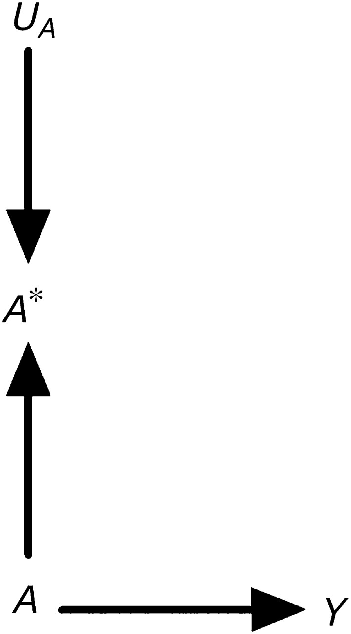
A causal directed acyclic graph representing a true exposure A, its measured version A*, and its measurement error U_A.

Figure 1 illustrates our assertion that measured exposures do not generally affect outcomes in observational studies. Clearly, A* has no direct or indirect causal effect on the outcome Y. However, A* is the only variable available to the investigator for estimating the effect of A on Y. The psychological literature sometimes refers to A as the “construct” and to A* as the “measure” or “indicator.” The challenge in observational disciplines is to make inferences about the unobserved construct (e.g., intelligence, statin use) by using data on the observed measure (e.g., intelligence quotient computed from questionnaire responses or estimated by factor analysis; information on statin use from medical records). The assumption implicit in many epidemiologic analyses is that the association between A* and Y approximates the association between A and Y. Unlike the situation in observational studies, in experiments one can generally argue that A* does have a causal effect on the outcome. For example, consider a double-blind placebo-controlled randomized clinical trial of statin use in which A* is an indicator of assignment to statin therapy and A is an indicator of actual statin use. The arrow from A to A* in Figure 1 would be reversed, and A* would have an indirect causal effect on Y mediated through A.

Besides the exposure A, the outcome Y may also be measured with error. The causal diagram in Figure 2, part A, includes the nodes Y* and U_Y, defined as the measured outcome and its measurement error. According to this graph, the errors for the exposure and the outcome are independent (11)—that is, f(U_Y, U_A) = f(U_Y) f(U_A), where f(·) is the probability density function. Independent errors might arise if, for example, data on both statin use A and liver toxicity Y were obtained from electronic medical records in which data entry errors occurred haphazardly. In other settings, however, the measurement errors for exposure and outcome may be dependent, as shown in Figure 2, part B. For example, dependent measurement errors might occur if the information on both A and Y were obtained retrospectively by phone interview and if a subject's ability to recall her medical history (U_AY) affected the measurement of both A and Y.

Figure 2.

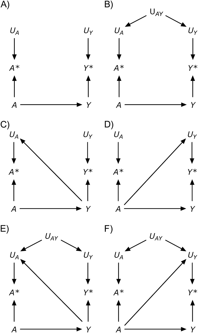
A structural classification of measurement error.

Both part A and part B of Figure 2 represent settings with nondifferential measurement errors (11): The error for the exposure is independent of the true value of the outcome—that is, f(U_A|Y) = f(U_A)—and the error for the outcome is independent of the true value of the exposure—that is, f(U_Y|A) = f(U_Y). Figure 2, part C, shows an example of independent but differential measurement error in which the true value of the outcome affects the measurement of the exposure (i.e., an arrow from Y to U_A). This type of measurement error might occur if the outcome Y were dementia rather than liver toxicity and statin use A were ascertained by interviewing study participants (because the presence of dementia affects the ability to recall A). A bias with the same structure might arise when estimating the association between blood lipids A and cancer Y if blood lipid levels are measured after cancer is present (because cancer affects the measured levels of blood lipids), or between alcohol use during pregnancy and birth defects when alcohol intake is ascertained by recall after delivery (because recall may be affected by the outcome of the pregnancy). Figure 2, part D, shows an example of independent but differential measurement error in which the true value of the exposure affects the measurement of the outcome (i.e., an arrow from A to U_Y). This type of measurement error might occur if physicians, suspecting that statin use A causes liver toxicity Y, monitored patients receiving a statin more closely than other patients. Parts E and F of Figure 2 depict measurement errors that are both dependent and differential, which may result from a combination of the settings described above.

In summary, Figure 2 depicts 4 types of measurement error: 1) independent nondifferential (part A), 2) dependent nondifferential (part B), 3) independent differential (parts C and D), and 4) dependent differential (parts E and F) (1). The description of measurement error in a causal diagram requires detailed knowledge of study design and procedures (2). It is important to keep in mind that causal diagrams do not encode quantitative information, and therefore they can be used to describe the structure of the bias but not its magnitude.

Epidemiologists study the association between measured exposures like A* and health outcomes like Y* even though they are aware that the measured exposure A* may not have a causal effect on the outcome. Studying the association between a measured exposure and an outcome in observational studies is an indirect way of assessing the effect of the true exposure on the true outcome. In the presence of dependent or differential measurement errors, this strategy is potentially biased because (as is easily concluded by applying the rules of d-separation (9)) the measured exposure A* is expected to be associated with the measured outcome Y* even under the null hypothesis of no effect of the true exposure A on the true outcome Y. We refer to the difference (in expectation) between the A-Y and A*-Y* associations as measurement bias or information bias, because the difference is due to the presence of measurement error.

In general, measurement error will result in bias. A notable exception is the setting in which A and Y are unassociated and the measurement error is independent and nondifferential: If the arrow from A to Y did not exist in part A of Figure 2, then both the A-Y association and the A*-Y* association would be null. In all other circumstances, measurement bias may result in an A*-Y* association that is either further from or closer to the null than the A-Y association. Worse, measurement bias may result in A*-Y* and A-Y trends that point in opposite directions. This trend reversal may occur even under the independent and nondifferential measurement error structure of Figure 2, part A (12), when the mean of A* is a nonmonotonic function of A (13). A more general theory on the direction of associations in causal diagrams has been recently proposed by VanderWeele and Robins (14).

Let us now return to the motivating example: the effect of BMI on a health outcome Y (5). It is widely accepted that some physiologic parameters related to body weight affect the risk of developing certain health outcomes. An exact characterization of these physiologic parameters is difficult, and thus they are sometimes (5) collectively referred to as “adiposity.” A key issue is how to provide a sharp operational definition of adiposity for epidemiologic research. Body weight is not, by itself, a good candidate for summarizing adiposity: A person weighing 80 kg may be considered obese if shorter than 1.60 m or underweight if taller than 2.05 m. It is not our goal here to summarize the vast literature on operational definitions of adiposity. Rather, we will focus on BMI, a deterministic function of measured height and weight, which is commonly used as a measurement of adiposity. The causal diagram in Figure 3 depicts, in addition to the construct adiposity A, the variables true body weight W, height H, and outcome Y; their corresponding measured versions W*, H*, and Y*; and their corresponding measurement errors U_W, U_H, and U_Y. Adiposity is depicted as a function of true weight W and height H, and the computed BMI* is depicted as a node with arrows only from both measured weight W* and height H*. This causal diagram is essentially equivalent to that proposed by Shahar (5), except that we allow for dependent measurement errors U_WH for weight and height.

Figure 3.

A simplistic causal directed acyclic graph for the association between body mass index (BMI) and a health outcome Y.

The causal diagram in Figure 3 is of course a gross, and likely incorrect, oversimplification of a complex issue. However, this graph suffices to show that the computed BMI*, like any other measured exposure, cannot possibly have a causal effect on the outcome Y. Additionally, under this causal diagram, the computed BMI* is associated with the measured outcome Y* only if adiposity A has a causal effect on the true outcome Y (i.e., if there is an arrow from A to Y). Therefore, one could argue that endowing the association between computed BMI* and measured Y* with an approximate causal interpretation as the effect of adiposity on Y is justified. This may be an implicit justification for the use of BMI in etiologic research. Note that this argument requires that measurement errors U_WH and U_Y be neither dependent nor differential. From this standpoint, BMI is no different from any other epidemiologic exposure.

There are other problems with BMI as an etiologic exposure that we do not discuss here: 1) BMI may not be the most appropriate characterization of adiposity (e.g., kg/m^2.5 might be a better choice, and fat tissue distribution may also be relevant); 2) BMI may need to be considered in conjunction with height (15); 3) effect-measure modification by BMI (or by weight W) is hard to interpret mechanistically if the causally relevant variable is the unobserved variable adiposity A; and 4) confounding adjustment is not straightforward for time-varying variables like BMI, especially when they are measured with error (16–18). Finally, the consistency assumption is particularly problematic when the goal is making causal inferences about the effects of BMI (or other functions of physiologic parameters) (19, 20). Note that lack of consistency does not mean that an arrow from A to Y cannot exist, as suggested by Shahar (5), but rather that hypothetical interventions on A are not well-defined, which may render causal inferences too vague to be useful for clinical or public health purposes.

In conclusion, exposures measured in observational studies may not have any effect on the outcome even if the underlying true exposures do. Further, the mere act of measuring variables (like that of selecting subjects) may introduce bias. Realistic causal diagrams of observational studies need to simultaneously represent biases arising from confounding, selection, and measurement.

Glossary

Abbreviation

BMI

body mass index

References

- 1.Hernán MA, Robins JM. A structural approach to observation bias [abstract] Am J Epidemiol. 2005;161(suppl):S100. [Google Scholar]
- 2.Robins JM. Data, design, and background knowledge in etiologic inference. Epidemiology. 2001;12(3):313–320. doi: 10.1097/00001648-200105000-00011. [DOI] [PubMed] [Google Scholar]
- 3.Hernán MA, Hernández-Díaz S, Werler MM, et al. Causal knowledge as a prerequisite for confounding evaluation: an application to birth defects epidemiology. Am J Epidemiol. 2002;155(2):176–184. doi: 10.1093/aje/155.2.176. [DOI] [PubMed] [Google Scholar]
- 4.Glymour MM, Greenland S. Causal diagrams. In: Rothman KJ, Greenland S, Lash TL, editors. Modern Epidemiology. 3rd ed. Philadelphia, PA: Lippincott Williams & Wilkins; 2008. pp. 183–209. [Google Scholar]
- 5.Shahar E. The association of body mass index with health outcomes: causal, inconsistent, or confounded? Am J Epidemiol. 2009;170(8):957–958. doi: 10.1093/aje/kwp292. [DOI] [PubMed] [Google Scholar]
- 6.Hernán MA. Confounding. In: Everitt B, Melnick E, editors. Encyclopedia of Quantitative Risk Assessment and Analysis. Chichester, United Kingdom: John Wiley & Sons; 2008. pp. 353–362. [Google Scholar]
- 7.Hernán MA, Hernández-Díaz S, Robins JM. A structural approach to selection bias. Epidemiology. 2004;15(5):615–625. doi: 10.1097/01.ede.0000135174.63482.43. [DOI] [PubMed] [Google Scholar]
- 8.Pearl J. Causal diagrams for empirical research. Biometrika. 1995;82(4):669–710. [Google Scholar]
- 9.Pearl J. Causation. 2nd ed. Cambridge, United Kingdom: Cambridge University Press; 2009. [Google Scholar]
- 10.Spirtes P, Glymour C, Scheines R. Causation, Prediction, and Search. 2nd ed. Cambridge, MA: The MIT Press; 2000. [Google Scholar]
- 11.Rothman KJ, Greenland S, Lash TL. Validity in epidemiologic studies. In: Rothman KJ, Greenland S, Lash TL, editors. Modern Epidemiology. 3rd ed. Philadelphia, PA: Lippincott Williams & Wilkins; 2008. pp. 128–147. [Google Scholar]
- 12.Dosemeci M, Wacholder S, Lubin JH. Does nondifferential misclassification of exposure always bias a true effect toward the null value? Am J Epidemiol. 1990;132(4):746–748. doi: 10.1093/oxfordjournals.aje.a115716. [DOI] [PubMed] [Google Scholar]
- 13.Weinberg CR, Umbach DM, Greenland S. When will nondifferential misclassification of an exposure preserve the direction of a trend? Am J Epidemiol. 1994;140(6):565–571. doi: 10.1093/oxfordjournals.aje.a117283. [DOI] [PubMed] [Google Scholar]
- 14.VanderWeele TJ, Robins JM. Signed directed acyclic graphs for causal inference. J R Stat Soc Series B. In press doi: 10.1111/j.1467-9868.2009.00728.x. [DOI] [PMC free article] [PubMed] [Google Scholar]
- 15.Michels KB, Greenland S, Rosner BA. Does body mass index adequately capture the relation of body composition and body size to health outcomes? Am J Epidemiol. 1998;147(2):167–172. doi: 10.1093/oxfordjournals.aje.a009430. [DOI] [PubMed] [Google Scholar]
- 16.Robins JM, Hernán MA. Estimation of the causal effects of time-varying exposures. In: Fitzmaurice G, Davidian M, Verbeke G, et al., editors. Longitudinal Data Analysis. New York, NY: Chapman and Hall; 2008. pp. 553–599. [Google Scholar]
- 17.Robins JM. Causal models for estimating the effects of weight gain on mortality. Int J Obes (Lond) 2008;32(suppl 3):S15–S41. doi: 10.1038/ijo.2008.83. [DOI] [PubMed] [Google Scholar]
- 18.Robins JM. General methodological considerations. J Econometrics. 2003;112(1):89–106. [Google Scholar]
- 19.Hernán MA, Taubman SL. Does obesity shorten life? The importance of well-defined interventions to answer causal questions. Int J Obes (Lond) 2008;32(suppl 3):S8–S14. doi: 10.1038/ijo.2008.82. [DOI] [PubMed] [Google Scholar]
- 20.Cole SR, Frangakis CE. The consistency statement in causal inference: a definition or an assumption? Epidemiology. 2009;20(1):3–5. doi: 10.1097/EDE.0b013e31818ef366. [DOI] [PubMed] [Google Scholar]