

Abstract
A method for the computation of low Reynolds number dynamic blood cell systems is presented. The specific system of interest here is interaction between cancer cells and white blood cells in an experimental flow system. Fluid dynamics, structural mechanics, six-degree-of freedom motion control and surface biochemistry analysis components are coupled in the context of adaptive octree-based grid generation. Analytical and numerical verification of the quasi-steady assumption for the fluid mechanics is presented. The capabilities of the technique are demonstrated by presenting several three-dimensional cell system simulations, including the collision/interaction between a cancer cell and an endothelium adherent polymorphonuclear leukocyte (PMN) cell in a shear flow.
Keywords: Computational Fluid Dynamics (CFD), Computational Structural Mechanics (CSM), Octree grid generation, Blood cells, Adaptive grid generation
1 Introduction
Flows with moving internal boundaries between different fluids and/or fluids and solid bodies are ubiquitous in nature and engineering. The computational analysis of these flows is more challenging than in single component flows due to the space-time evolution of internal boundaries, as well as discrete interface resolution requirements and associated boundary/jump conditions. In the past several decades, a number of methods for simulating flows with multiple moving bodies and interfaces have been formulated and refined. Such methods and analyses have appeared in literature as diverse as (but not limited to) aerospace (Togashi et al., 2003) and civil (Hu, Patankar, and Zhu, 2001) engineering, and biology (Mulholland et al., 2005; Leroyer and Visonneau, 2005; Cardoze et al., 2004). Biological systems typically present additional challenges associated with complex and difficult to define geometries, and complex constitutive relations associated with both the fluid and solid constituents of the system under study. Methods for computational modeling of flows with moving internal boundaries have been surveyed by several authors, including Osher and Fedkiw, 2003, Hu, Patankar, and Zhu, 2001, Shyy et al., 2001, Dong and Lei, 2000, and Lei et al., 1999. A brief summary of pertinent techniques is presented here.
Three classes of CFD methods are employed in multi-component systems: 1) Eulerian, or front capturing, methods where the interface is implicitly accounted for through the introduction of a transport field variable, 2) Lagrangian, or front tracking, methods that employ moving grids whose vertices lie explicitly on the interfaces, and 3) combined Lagrangian-Eulerian methods. In Eulerian methods, the governing equations are solved on nominally stationary, non-interface-fitted and often (but not exclusively) Cartesian grids, and a transport field variable is used to implicitly account for the interface. These front capturing methods (Osher and Fedkiw, 2003) simplify grid generation significantly. However, the influence of the interface on the surrounding fluid may be smeared across several grid elements (Shyy et al., 2001). Volume-of-fluid (VOF) (Hirt and Nichols, 1981) and level-set methods (Osher and Sethian, 1988) are well established examples in this class. The Eulerian methods lack an obvious method of applying boundary conditions to the discrete differential operators themselves, and this makes the effect of their application unknown on the accuracy of the solution (Mittal and Iaccarino, 2005).
In Lagrangian methods, moving and/or topologically adaptive grids conform in space and time to the evolving geometry of the system's internal interfaces, which can become quite complex even in simple applications (Osher and Fedkiw, 2003). These methods have been used to model prescribed motions of interfaces by generating meshes of varying configurations prior to the simulation (Mulholland et al., 2005; Leroyer and Visonneau, 2005). Moving overset grids (Belk and Maple, 1995; Freitas and Runnels, 1999) and adaptive unstructured grid methods (Cardoze et al., 2004) are two techniques in this class. An adaptive grid, front tracking method is used in this work.
Lagrangian-Eulerian methods combine the advantages of stationary grid and interface tracking grid methods. Specifically, the governing equations are solved on a non-interface fitted background (usually Cartesian) grid, as in Eulerian methods, and an interface-fitted grid is overlayed with the background grid to explicitly track the interface. For example, the immersed finite element method (IFEM) was recently developed (Zhang, 2004; Liu et al., 2006) to improve upon a widely used technique in this class, the immersed boundary method (IBM) (Peskin, 2002; Mittal and Iaccarino, 2005). The combination of a Cartesian background mesh with an overlapping boundary mesh is the basis of both methods. These methods ameliorate the smearing effect of the Eulerian methods while retaining simplified grid generation.
The present work focuses on the application of an adaptive mesh technique in the direct numerical simulation (DNS) of systems of blood cells. In DNS methods, all flow dynamics and particle motions are discretized simultaneously, and therefore they are capable of fully resolving the physics of particle-fluid, particle-particle and particle-wall interactions (Hu, Patankar, and Zhu, 2001). DNS methods can be computationally intensive, especially at high Reynolds numbers where the range of scales to be resolved can render direct simulation prohibitive. However, these methods become tractable for the low Reynolds number laminar flows that arise in small blood vessels. Accordingly, we employ DNS in this work.
The specific system under study here is cancer cell - white blood cell interaction near a wall in a shear flow (Slattery, Liang and Dong, 2005; Liang, Slattery and Dong, 2005; Dong et al., 2005). The interactions between these cell types may be involved in the process of cancer metastasis, or the spread of cancer through the body. Experimental observations of PMN-cancer cell adhesion indicate that PMNs are significantly more deformable than cancer cells and that cancer cells are likely to adhere to PMNs that have already attached to the substrate (Liang, Slattery and Dong, 2005). Computational models of blood flow and blood cells have been developed for a wide range of biological applications, including thrombosis (Pivkin, Richardson, and Karniadakis, 2006), inflammation (Khismatullin and Truskey, 2005; King and Hammer, 2001; Dong et al., 1999; Cao et al., 1998), and white blood cell deformability (Dong et al., 1991; Dong and Skalak, 1992; Dong and Lei, 2000; Kan et al., 1998). To the authors' knowledge, the cancer cell-white blood cell system studied here has not been previously modeled.
Two-dimensional models of white blood cell deformability have been developed previously using Lagrangian methods. For example, Dong et al. calculated the cell internal and external flow fields using finite element analysis, and calculated the interface deformation using membrane equations (Lei et al., 1999; Dong and Lei, 2000). However, the majority of researchers modeling white blood cells in flow have used Eulerian or combination Lagrangian-Eulerian methods. For example, Khismatullin and Truskey, 2005, used a VOF method to simulate deformable white blood cells as they adhere to surfaces. N'Dri, Shyy, and Tran-Son-Tay, 2003, also simulated the attachment of white blood cells to surfaces using an IBM. King and Hammer (2001) used a completed double layer boundary integral equation method (CDL-BIEM) to simulate spheres or white blood cells adhering to a flat surface in a shear flow. These researchers elucidated the complexity of modeling deformable cells.
In this work, an octree-based adaptive mesh Lagrangian method is developed and demonstrated to be both efficient and accurate. Computational Fluid Dynamics (CFD), Computational Structural Mechanics (CSM), biochemical kinetics, and six-degree-of-freedom motion control (6DOF) are coupled in the context of adaptive grid generation to simulate a cellular system. Commercial software is used for the CFD, CSM, and mesh generation components, and author-developed software is used for the biochemistry and 6DOF components, and to couple the overall analysis procedure. The coupled strategy is demonstrated by modeling a rigid cancer cell interacting with both rigid and deformable, wall-adherent white blood cells corresponding to conditions of an experimental system.
The paper is organized as follows: The governing equations for the fluid dynamics, structural mechanics, biochemical interactions and motion control are described first. Details of the numerics and software coupling for the method are then presented. Verification and validation of the method are discussed and the results of two computational studies are presented.
2 Theoretical formulation
The method presented here involves the implementation and coupling of four component technologies. The governing equations for each of these; fluid mechanics, structural mechanics, biochemical interactions, and six-degree-of-freedom motion, appear here. The coupling of these physics through flow and surface biochemistry forces are then summarized and the overall analysis approach is outlined.
2.1 Governing equations
2.1.1 Fluid dynamics
The governing equations for the flow are the incompressible Navier-Stokes and continuity equations:
| (1) |
| (2) |
where the flow is assumed to be Newtonian and of uniform viscosity:
| (3) |
In this set of equations, vi is the velocity vector, xi is the coordinate vector, ρ and μ are the fluid density and viscosity, p is the pressure, and τij is the stress tensor.
2.1.2 Structural mechanics
Qualitative observations of cancer cell-white blood cell interactions indicate the cancer cells are significantly less deformable than white blood cells (Liang, Slattery and Dong, 2005), thus the structural mechanics equations are solved here for the PMN only. The deformable PMN is modeled as a three-component system that includes a viscoelastic cytoplasm, an elastic membrane, and a rigid nucleus, as shown in Figure 1.
Figure 1.
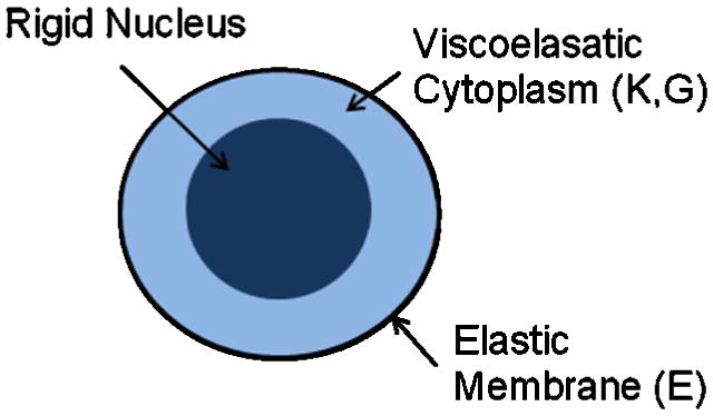
Schematic representation of the three-component deformable PMN model.
For the cytoplasm, the governing equation is the hereditary integral formulation for a linear, isotropic viscoelastic material (Darby, 1976):
| (4) |
where G is the shear modulus, K is the bulk modulus, ed is deviatoric strain, ev is volumetric strain, and the dot represents differentiation with respect to time.
In the quasi-steady approach used for all of the simulations presented herein, a time accurate, static, stress/displacement analysis is run in Abaqus to solve for the time-dependent material response. For these simulations, the bulk modulus, K, and the shear modulus, G, for the cytoplasm, and the elastic modulus defined for the membrane are each specified as time-independent constants.
The viscoelastic constitutive relation is used for all volume elements of the PMN except those within a sphere comprising 20% of the cell volume, which were defined to be part of a rigid body. This rigid nucleus was defined in the center of the PMN such that forces from the cytoplasm were applied only to the center of the rigid body and the elements maintained a constant separation from each other.
A linear, isotropic membrane was defined using the shell elements surrounding the cell. The governing equation for the elements of the membrane is the simplified linear equation of an elastic material (Darby, 1976):
| (5) |
where E is the elastic modulus and ε is the total elastic strain. For the membrane, only in-plane stresses are considered and an initial tension, or prestress, is applied as in (Dong et al., 1988).
2.1.3 Biochemical interactions
It is possible for cancer cells to adhere to white blood cells via molecular interactions. Adhesion molecules that protrude from the cells' surfaces can interact and join to form bonds. The formation and breakage of individual bonds are governed by a probability during each time step (Hammer and Apte, 1992):
| (7) |
where P represents the probability that a bond will form or break in a time step of length Δt. The constant, k, represents one of the constants, kon or koff, that govern the rate at which bonds form or break, respectively. These constants are calculated based on Bell's kinetics theory and extensions thereof (Hammer and Apte, 1992; Bell, 1978):
| (8) |
| (9) |
The constants, k0on and k0off, are the rates that a bond will form or break under equilibrium conditions. The rates used here were derived experimentally by two of the authors in a companion effort (Hoskins and Dong, 2006) for the binding of the adhesion molecule, ICAM-1, on cancer cells with LFA-1 and Mac-1, two compatible adhesion molecules, on white blood cells. The adhesion molecules, and formed bonds, are treated as linear springs with spring constants s and sts and an equilibrium length of λ. Values for the constants s, sts and λ, as well as the number density of LFA-1 or Mac-1 molecules on the white blood cell surface, nL, were obtained from Dembo et al., 1988, and Simon and Green, 2005. The value of d, the separation distance, AL, the surface area available for bond formation and nB, the number density of bonds, are determined from the state of the system at any given time step (see Section 2.4.4). The number density of ICAM-1 molecules is used to determine how many potential bonds may form during a time step (see Section 2.4.4).
2.1.4 Six-degree-of-freedom motion dynamics
The in vitro system modeled here consists of the interaction of a cancer cell with a white blood cell bound to the bottom wall of a test chamber (see geometry in Figures 6, 8, 9). For this system, the motion of the cancer cell is governed by six-degree-of-freedom (6DOF) motion control, or Newton's Law, equations:
Figure 6.
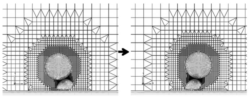
Example meshes of the cancer cell-white blood cell system. The large spherical particle is the cancer cell and the smaller deformed particle represents the white blood cell. A clip plane through the center of the three-dimensional mesh and the surface grids are shown.
Figure 8.
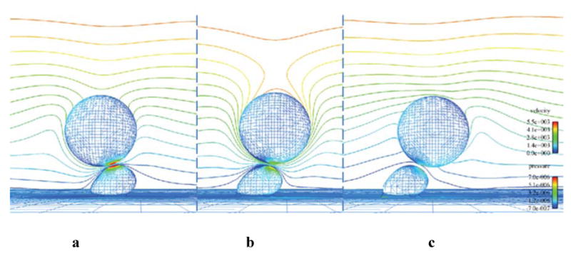
CFD results for three time points during the biochemistry simulation a) 4.5 ms, b) 8 ms, c) 9.8 ms. The cell surfaces are contoured by pressure and the far-field symmetry plane is contoured by velocity magnitude. Flow direction is left to right.
Figure 9.
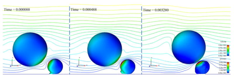
Three time steps in the simulation of a collision between a rigid cancer cell and a deformable white blood cell showing the peeling motion of the white blood cell. The cells are contoured by pressure (in kg/μm-s2) and a center clip plane is contoured by velocity magnitude (in μm/s). Flow direction is left to right.
| (10) |
| (11) |
Here xi is the translational displacement of the cell center of mass, θi is the rotational displacement around the center of mass, Fi is the sum of the fluid and interaction forces applied at the cell center of mass, τi is the torque applied to the cell center of mass, m is the mass of the cell, and I is the moment of inertia of the assumed spherical cancer cell. (The form of equation 11 is valid with scalar moment of intertia, I, due to the assumption that cancer cells are rigid spheres.)
2.2 Fluid-structure-biochemistry coupling
The forces and torques that ultimately define the PMN geometry and the cancer cell motion arise from fluid forces (pressure and viscous) and interaction forces (repulsion and adhesion). For the 6DOF motion, all of the forces and torques are resolved to the cancer cell center of mass before the 6DOF motion equations are solved. For the PMN deformation, the nodal fluid forces computed by AcuSolve are applied to the surface nodes in the Abaqus PMN mesh. The repulsion and adhesion forces are not applied to the PMN during the deformation computations under the assumption that the fluid forces dominate the deformation response. This is a simplifying assumption whose accuracy is discussed in the Conclusions section.
The fluid forces on the cells are computed from the area integration of the pressure and viscous stresses:
| (12) |
where p is the pressure and nˆi is the outward normal vector to the surface. Moments are calculated by integrating the cross product of the surface element forces with the vector distance of the element to the origin.
A repulsion force is applied to the cancer cell when it approaches the white blood cell due to the existence of small protrusions, termed microvilli, that extend from real cell surfaces. Several different forms of this force have been used in simulations presented by other researchers (Bongrand and Bell, 1984; Migliorini et al., 2002). Here the repulsion is modeled using a simple non-linear spring force, with the general form:
| (13) |
The distance between the smooth cell surfaces is represented by ds and the constants a and b are set such that a small gap was maintained to account for the microvilli (the minimum gap between the cells is approximately 0.3 μm).
The separation distance, ds, is the harmonic average of the minimum separations between surface nodes on the cells. The repulsive force is applied at the point of minimum separation on the cancer cell along the normal to the PMN surface at the point of minimum separation on the PMN, nˆi. The force is applied to the cancer cell center of mass and since that line, in general, does not pass through the center of the cancer cell, the corresponding moment is also applied.
Bonds are modeled as linear springs (Hammer and Apte, 1992), thus the adhesion forces and moments are calculated using Hooke's Law:
| (14) |
Here, Fb,j is the bond force applied by a single bond, s is the linear spring constant (Dembo et al., 1988), and êj is the unit vector denoting the line of action of the bond. In the time step in which the bond is initially formed, the line of action is in the direction of the minimum surface-surface separation. In subsequent time steps, the line of action is recalculated due to the movement of the cancer cell. The difference between d and λ is the departure from the bond's equilibrium distance. The calculation of d is described in Section 2.4.4.
2.3 Quasi-steady approach
The quasi-steady approach used here is defined by neglecting time dependence in the Navier-Stokes equations, while retaining it in the motion control and structural mechanics equations. The low Reynolds numbers and the rapid response time of cells in these systems make this valid. By discarding the time derivative terms in the Navier-Stokes equations, the requirement for mesh topology consistency on successive time steps is eliminated.
To verify that this quasi-steady approach is accurate for the cellular systems of interest here, an analysis due to Brennan, 1995, is adapted. We consider a cancer cell flowing past a white blood cell bound to the bottom wall of a test chamber. The carrier fluid is a water-like, Newtonian fluid with the same density and viscosity as blood plasma. The relevant Reynolds number of this system is based on the average chamber flow velocity, U, and the cancer cell radius, R:
| (15) |
A size parameter is also defined (Brennen, 1995):
| (16) |
where l is the typical length dimension in the system; here we use a representative mean diameter of the white blood cell that the cancer cell is flowing past. The densities, ρc and ρf, are of the cell and the carrier fluid, respectively, and the viscosity, μ, is that of the fluid. For the highest Reynolds number of interest here we have:
U = 0.0042 m/s
R = 8 μm
l = 10 μm
ρc = 1087 kg/m3
ρf = 1000 kg/m3
μ = 0.001 kg/m · s
The Reynolds number and size parameter are approximately 0.0336 and 0.07, respectively. These values put the system of interest in the quasi-steady regime (Brennen, 1995), which indicates that a quasi-steady approximation is accurate. This is verified numerically in Section 4.1.
2.4 Numerics
2.4.1 CFD
The commercial software package, AcuSolve (ACUSIM Software, Inc.), is used to solve the governing fluid dynamics equations. AcuSolve employs a Galerkin Least Squares (GLS) discretization formulation (Jansen et al., 1999). A Newton class method is used to solve the coupled nonlinear continuity and momentum equations in their weak form (Jansen et al., 1999):
| (17) |
where index k designates the equation (k=1, continuity; k=2, momentum), Wk are piecewise linear weight functions (that render the discretization second order accurate in space and time), Fki are the sum of inviscid and viscous fluxes for equation k in the ith coordinate direction, V is the spatial domain of the problem bounded by closed surface A, and Ve are the individual discrete finite elements into which V is decomposed. The first two terms in equation 17 represent the Galerkin approximation. The last term contains the least-squared stabilization characterized by Lij, the Jacobian matrix of the linearized temporal, convection and diffusion operators, and τij, the Least Squares stabilization matrix. Further details on the formulation of the method can be found in (Johnson and Bittorf, 2002; Jansen et al., 1999).
In the context of the quasi-steady approach, the Navier-Stokes equations are solved on a new grid every physical time step by running AcuSolve in steady state mode. Convergence tolerance was set such that the forces and moments converged to three significant digits.
2.4.2 Structural mechanics
The commercial software package, Abaqus/Standard (Simulia), is used to solve the governing structural mechanics equations. Abaqus employs a displacement based finite element analysis formulation. Newton's method is used in increments to solve the nonlinear equilibrium equations in their weak form (Darby, 1976):
| (18) |
where V is the volume of a differential element at the current time and S is the surface bounding that element. δvi is the “virtual velocity field” or “test function”, δDij is the virtual strain rate tensor conjugate to the stress matrix, σij, ti is the surface traction on S, and fi is the body force on the volume. A standard finite element interpolator is applied to these equations to solve for the system variables at equilibrium.
2.4.3 Grid generation
The commercial grid generation package, Harpoon (Sharc Ltd.), is used to generate meshes for both the CFD and CSM analyses. Harpoon uses an octree technique to mesh geometry using user-defined element size constraints. An octree is generated by recursively dividing “parent” hexahedral elements along each axis to create eight equal-sized “child” elements (De Zeeuw and Powell, 1993). Harpoon first creates a “root” hexahedral element that encompasses the flow domain. The root element and its children are then refined continuously until the user-defined coarsest allowable element size on each surface is obtained. Harpoon uses a hex-dominant technique, meaning geometry around a boundary is closely approximated using hexahedra, then to more accurately capture surface geometry, tetrahedral, prism and pyramid elements are added. This octree method has been observed here to be fast (a 150,000 node mesh can be created in less than 20 seconds on a desktop PC), robust to complex system geometries, and easily automatible through its batch mode capability.
At each time step, the flow domain (blood vessel or in vitro test chamber) and cells within the domain are meshed such that vertices are located on the cell membranes. The mesh of the interior of the deformable cell is saved for the structural mechanics simulation and the mesh of the fluid regions is saved for the fluid dynamics simulation. By generating both meshes at once, the surface topology is conserved and interpolation of deformation and force results is unnecessary. When cells are close to each other or to a wall, the gap between them is refined using refinement zones. A refinement zone is defined in Harpoon by a geometric shape (sphere, trapezoid box, etc), inside which grid elements are refined to a user-defined level. In the context of multiple cell simulations, adaptive refinement zones are generated by constructing a trapezoid box around the line that traverses the shortest distance between cells or between a cell and a wall (illustrated in Figure 6). The refinement zone is generated in order to ensure a sufficient number of grid elements remains within the gap between the cells. Since the flow is laminar and AcuSolve uses a second order accurate element-centered discretization, three elements were required between the cell boundaries. This amount of refinement was also determined to be sufficient in test simulations.
2.4.4 Biochemistry
Coding developed by the authors is used to implement the probabilistic biochemistry model described in Section 2.1.3. At every time step, a single bond formation is considered. If the probability of bond formation, calculated using equations 7 and 8, is greater than a random number generated between 0 and 1, a bond is formed. Formed bonds are treated as linear springs and the bond force is calculated using equation 14. Once bonds form, they are tested in subsequent time steps for breakage. If the probability of bond breakage, calculated using equations 7 and 9, is greater than a random number between 0 and 1, then the bond breaks. The probability that the bond will break increases as the bond length, d, deviates from the equilibrium bond length, λ.
To calculate the probability of bond formation, d and AL need to be calculated. Actual cell surfaces are not smooth, but contain protrusions and microvilli of varying lengths [95% are less than 0.5 μm long (Bruehl, Springer and Bainton, 1996)]. This surface roughness is modeled here by assuming a random distribution of rigid, normal protrusions on the smooth cell surfaces between 0 and 0.5 μm in length. The separation distance, d, is calculated as the distance between these roughness elements on colliding cells (or d = ds − dr, where dr is the total length of the roughness elements on both cells). It is considered that an adhesion molecule at the tip of the roughness elements may interact with the adhesion molecules on the opposing cell. Thus, the interaction area, AL, is assumed to be a circular area with radius equal to the surface protrusion length on the cancer cell at that time step.
The probability of bond formation is compared to random numbers that are generated for each potential bond in a time step. It is assumed that all adhesion molecules within the interaction areas of two cells could potentially bind with each other. Therefore, the number of potential bonds (and thus the number of random numbers generated in a time step), NR, is:
| (20) |
where nL and nI are the number densities of LFA-1 or Mac-1 and ICAM-1 molecules on the white blood cell and cancer cell surfaces. One of either LFA-1 or Mac-1 is considered for bond formation during a single time step. A random number between 0 and 1 is compared to the ratio of LFA-1 and Mac-1 surface densities to determine which molecule may bind with ICAM-1 during that time step.
2.4.5 Six-degree-of-freedom motion
A second order accurate one-sided explicit method was used to discretize the equations of motion for the cancer cell (equations 10 and 11):
| (21) |
| (22) |
Here ′ represents differentiation with respect to time and superscripts n and n−1 represent the current and previous times. The second derivative of x and θ are calculated using Newton's Law, thus x″n-1 = Fn-1 / m and θ″n-1 = τn-1 / I. Through numerical experimentation, this second order method was found to return nearly time step invariant cell trajectories with a time step size of 8 μs. This observation is consistent with the estimated response time, tR, for a particle (Brennen, 1995) applied to this system:
| (23) |
Specifically, taking ρf, ρc, R, and μ as in section 2.3, the response time for the cancer cell is computed to be approximately 20 μs.
Prior to the adoption of equations 21 and 22, first order (Euler explicit) and 4-stage Runge-Kutta (RK4) schemes were explored for solving the dynamics equations. The Euler explicit scheme required smaller timesteps (for stability) than required for the second order explicit scheme. Also, unlike our experience in high Reynolds number flows, the RK4 method was not found to be more stable or efficient than the one-sided difference used.
In further numerical tests of cancer cell motion, the maximum change in cell velocity during a time step was approximately 100 μm/s in any direction. However, when a bond formed, the maximum change in velocity during a time step was approximately 650 μm/s. Accordingly, the time step size was decreased to 1 μs when a bond was formed.
3 Software coupling
The overall strategy for the simulations is displayed schematically in Figure 2. The operations shown in the schematic are controlled by an author-developed Python script. The model is capable of simulating the interaction of an arbitrary number of cells, each with or without deformation, and with or without bond biochemistry.
Figure 2.
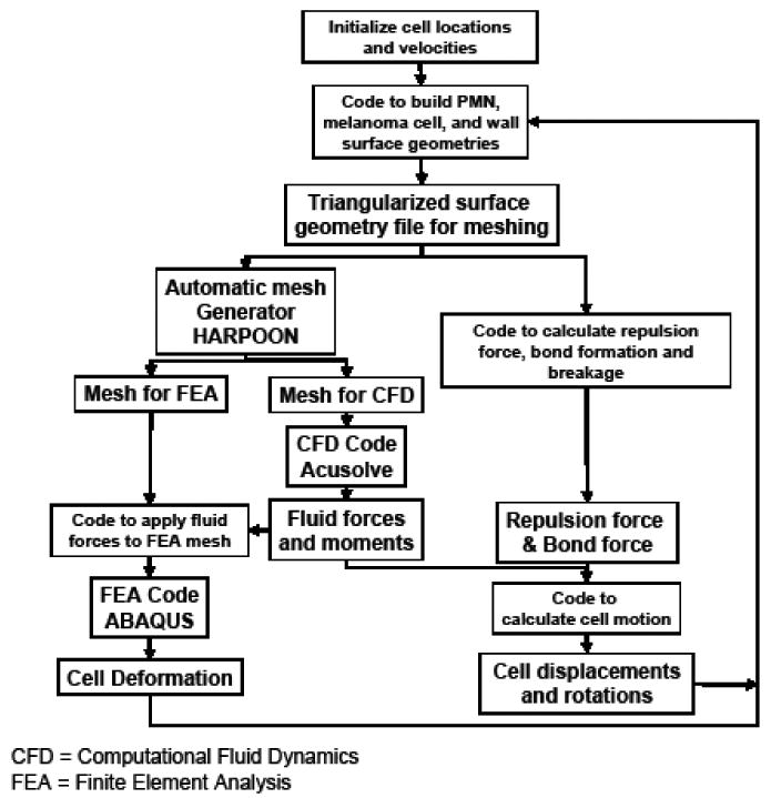
Schematic representation of the software infrastructure.
To start the simulation, the Python script is initialized with the channel dimensions, user-defined starting cell positions and shapes, and any existing bond locations. At each time step, a FORTRAN 77 code is run that generates and outputs an STL file of the triangularized surface geometry. In the first time step, the geometry corresponds to the user-defined starting cell geometry. In subsequent steps, the cell locations are those computed by the 6DOF motion equations. The code also computes the inter-cellular distance and the corresponding repulsion force, and completes the bond formation and breakage tests for the current system geometry. The bond and repulsion forces are then summed and stored to be applied to the motion control calculation.
Harpoon is then invoked to generate a mesh with fluid and cell elements stored separately. The AcuSolve input file is then edited automatically by the Python script to include appropriate boundary conditions and run controls. Nodal pressures and velocities from the previous time step's CFD solution are projected onto the nearest node of the new mesh, to supply an initial guess for the next simulation, which decreases the CFD run times. The CFD analysis is then run in steady state mode and the computed forces and torques on the cancer cell surface are stored for later use.
The Abaqus input file is next edited to include: loads on each surface node corresponding to the nodal surface forces from the CFD analysis, motion constraints on the necessary nodes, a rigid body definition for the nucleus of the white blood cell, material properties, and run control inputs. The CSM analysis is then run and the computed deformations of the surface nodes are output to a file.
The fluid, repulsion, and bond forces on the cancer cell are then totaled in the control script, where the motion control equations themselves are solved for the cell translations, rotations, and velocities. That information and the CSM deformations are then passed back to the initial FORTRAN 77 code, which generates a new STL file and begins the next time step. This process is repeated until the user-defined number of time steps are completed.
4 Results
4.1 Verification and validation
Several preliminary studies were completed, including simulations of single, stationary cells and two-dimensional moving cells, which led to the method described herein. These studies, presented in this section, were conducted using an alternative CFD solver, NPHASE-PSU (Kunz et al., 2001). Like AcuSolve, NPHASE-PSU employs second order accurate discretization numerics, but unlike AcuSolve, supports overset mesh topologies required below. By virtue of its segregated solution strategy, NPHASE-PSU is less efficient than AcuSolve (which employs a fully implicit pressure-velocity coupling) for very low Reynolds number flows; thus AcuSolve was used for the full scale simulations presented in Sections 4.2 and 4.3. No significant differences were observed in the results when the solvers were compared in representative steady simulations of a white blood cell-cancer cell system.
In earlier work (Leyton-Mange et al., 2006), grid and validation studies were completed in the present low Reynolds number regime. Briefly, when a single spherical particle in a semi-infinite flow was simulated with a grid of approximately 175,000 elements at a Reynolds number of 0.1, Stokes Drag Law was returned within 1 percent. In another study, the flow field around a single, deformed, but rigid, stationary cell, inside an experimental flow chamber geometry was computed, and numerical results were found to compare favorably with experimental measurements of the same system (Leyton-Mange et al., 2006). Specifically, the experimental and numerical velocity profiles agreed well, as shown in Figure 3, and described in detail in Leyton-Mange et al., 2006.
Figure 3.
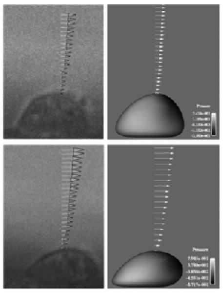
Velocity profiles above a single cell under low (top) and high (bottom) shear rates from the solver validation test.
To verify the enabling quasi-steady assumption made in this work, the fluid forces on a moving cancer cell were computed during a transient simulation and compared to those computed in discrete steady simulations of the same motion. To accomplish this, a two-dimensional model was generated of a stationary, deformed white blood cell and a rigid cancer cell in a rectangular flow channel using two-dimensional overset grids. Specifically, one mesh was constructed for the PMN + channel geometry, and another mesh was constructed for, and moved with, the cancer cell (Figure 4.) Overset meshes were used for this study since mesh topology is retained in successive time steps, and therefore a conservative discretization of the time-dependent Navier-Stokes equations could be performed. The grids were compiled and allowed to inter-communicate within the flow solver using the overset mesh assembly and communication software, SUGGAR (Noack, 2005) and DiRTlib (Noack, 2005).
Figure 4.
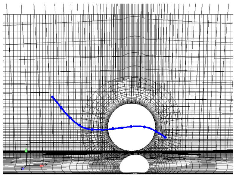
System of two-dimensional overset grids used for the quasi-steady assumption verification simulations. Solid line represents the path of the cancer cell in the simulations.
Motion was prescribed for the cancer cell center of mass such that it traversed a cubic displacement path around the white blood cell, as illustrated by the line in Figure 4. Sixty-two time steps were taken, for a total simulation time of 0.22 ms. For comparison, twelve steady state simulations were also performed, where the cancer cell was placed in locations along the prescribed path, and appropriate velocity boundary conditions were defined on the cancer cell surface. The Reynolds number based on the relative velocity of the cell (Vcell − Vflow) was approximately 0.0667.
The drag and lift forces on the cancer cell surface calculated in the transient and steady simulations agreed very well, as shown in Figures 5a and b. Qualitatively, the velocity and pressure profiles were also nearly identical (not shown). This test confirmed that the transient terms in the Navier-Stokes equations are negligible and the quasi-steady technique presented herein is valid for the system of interest.
Figure 5.
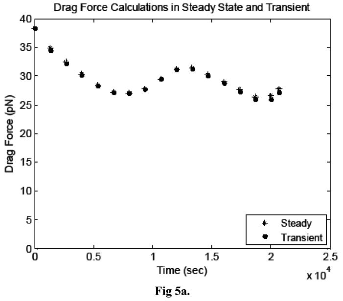
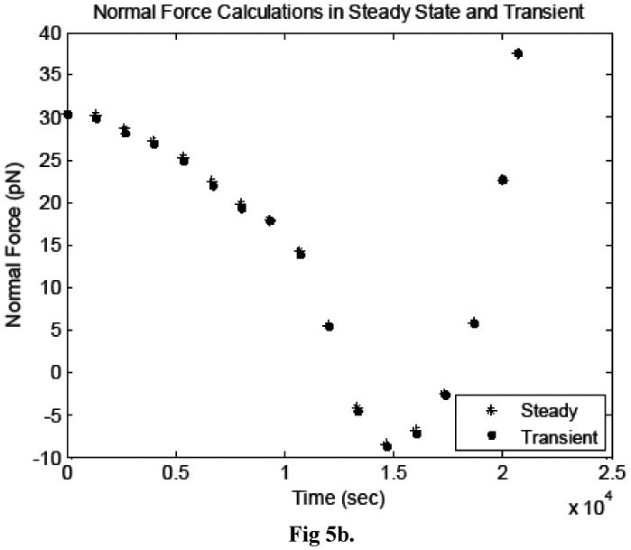
Comparison of the a) drag forces and b) lift forces acting on the cancer cell, calculated in transient and steady simulations.
4.2 Cancer cell-white blood cell interaction
4.2.1 Adhesion verification
The interaction of a rigid, spherical cancer cell with a rigid, deformed white blood cell was simulated. The six-degree-of-freedom motion, adhesion kinetics, and fluid dynamics governing equations were all solved, as described in Section 2. Simulations were performed in which adhesion was and was not considered.
The cancer cell was placed at an arbitrary initial location upstream of the white blood cell in an experimental flow chamber with a rectangular cross-section. The full length (2 cm) and width (2.5 mm) of the actual in vitro flow chamber were not modeled, but the mesh extended 8 cell diameters upstream, downstream, and on each side of the cell. This is sufficient since, at the low Reynolds numbers considered here, entrance effects are negligible with the flow becoming fully developed very rapidly. The full height of the chamber (127 μm) was modeled. The upstream boundary was assigned an inlet velocity profile defined using the mean chamber flow velocity and assuming a Poiseuille flow between parallel plates. A mean chamber velocity corresponding to a wall shear rate of 200 s-1 was specified. The fluid viscosity of 0.001 kg/m·s was used in these simulations. The downstream wall was assigned a constant pressure condition, the top and bottom walls were assigned a no-slip condition, and the side walls were assigned a symmetry condition. A simplified adhesion model was applied, in which LFA-1 only was considered to form bonds with ICAM-1 and the area of interaction was set to a constant value for the full simulation. The number of LFA-1 and ICAM-1 molecules on the cell surfaces corresponded to resting white blood cells (45 LFA-1 molecules/μm2, Simon and Green, 2005) and the melanoma cell line WM-9 (13 ICAM-1 molecules/μm2, Courtesy of Shile Liang).
Similar to the steady simulations of cancer cell motion in the verification study described in the previous section, velocity boundary conditions were applied to the cancer cell surface equal to the velocities from the previous time step's 6DOF calculations. When the gap between the two cells was small, a refinement zone was added to ensure sufficient grid refinement between the cells' surfaces. Grids generated for the simulation at different time steps ranged from 180,000 to 250,000 elements, depending on this refinement and the cell locations. An example grid generated during the simulation is shown in Figure 6, illustrating the grid adaptation as the cancer cell traversed the white blood cell.
Figure 7a compares the cell separation distance time histories in both simulations and Figure 7b shows the time history of number of formed bonds. The erratic motion of the cancer cell, illustrated in Figure 7a, is a well-documented behavior of cells attaching to other cells via molecular bonds (House and Lipowsky, 1988, for example) and is attributed to the stochastic nature of bond formation and breakage, which is modeled here. The images in Figure 8 show pressure and velocity contours computed at three time steps. The first shows the system at approximately 4.5 ms, as the number of bonds peaked the first time. The second image is at 8 ms, and the third is the last time step calculated during the simulation, at approximately 9.8 ms. It is evident from Figure 7 that the cancer cell path and velocity were significantly altered due to molecular bond forces.
Figure 7.
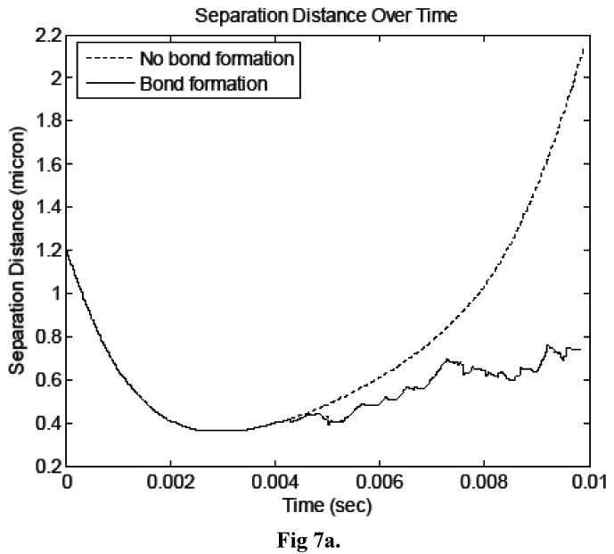
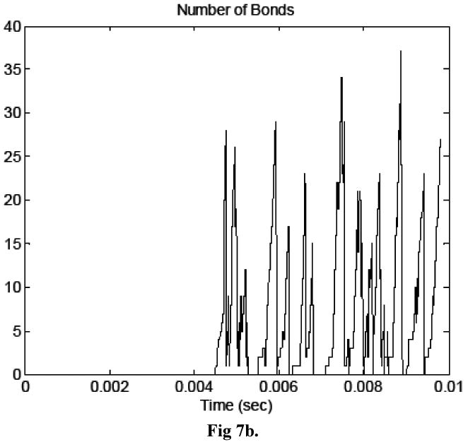
a) Time history of cell separation distance for simulations in which bonds did and did not form. b) Time history of number of bonds in the simulation in which bonds formed.
The inclusion of the biochemistry does not add significant run time to each step, however the decrease in time step size when bonds formed adds to the number of time steps necessary to complete the simulation. Just over 4200 time steps were completed in the biochemistry simulation, which took approximately 325 hours on four 2.33 GHz Intel quad-core Clovertown processors. The same simulation without bond formation required 1230 time steps and approximately 100 hours.
4.2.2 Deformable white blood cell
The interaction of a rigid, spherical cancer cell with a deformable white blood cell was also simulated. The six-degree-of-freedom motion, adhesion kinetics, structural mechanics, and fluid dynamics governing equations were all solved, as described in Section 2. Two simulations were performed, one in which adhesion was modeled and one in which it was not.
A deformable, PMN was modeled on the bottom of the same rectangular chamber described in the previous section, and a rigid melanoma cell was initially placed upstream. As in the previous section, a shear rate of 200 s-1 and a viscosity of 0.001 kg/m · s were used in these simulations, and the same boundary conditions were applied. The melanoma cell and PMN were initialized as spheres in their starting locations. The white blood cell had an initial radius of 3.5 μm and the cancer cell radius was 8 μm.
The deformable white blood cell structural model consisted of three components as shown in Figure 1. The majority of the cell was considered a viscoelastic solid with governing equations described in Section 2.4.2. The bulk modulus, K, was set to 5682 Pa, Poisson's ratio, ν, was set to 0.499 to model incompressible behavior, and the shear modulus, G, was set to 1894 Pa (G = K/(2(1+ ν))). The value of bulk modulus was set to yield cell shapes consistent
A rigid, spherical nucleus was defined in the center of the white blood cell that contained 20% of the total cell volume. The elastic membrane was defined as in (Dong et al., 1988) with an elastic modulus of 150 Pa, a 0.1 μm thickness, and an initial stress of 31 μN/m. The white blood cell was assumed to be rolling on the bottom wall in a peeling motion. This was modeled by un-constraining 15% of the length of the cell on the trailing side.
Figure 9 shows three time steps of the initial PMN motion to demonstrate the peeling motion.
The binding of LFA-1 and Mac-1 with ICAM-1 was modeled here, as described in Section 2.4.4. The LFA-1 and Mac-1 surface densities on white blood cells used were determined in a companion study (210 LFA-1 molecules and 105 Mac-1 molecules per μm2) and the ICAM-1 surface density on cancer cells was consistent with a cell line used in experiments (WM-9 cells, 13 ICAM-1 molecules per μm2).
The time history of bond formation during the simulation is shown in Figure 10. For comparison, a simulation was also carried out in which bonds were prohibited from forming between the cells, with the remaining model parameters unchanged. Figure11 compares the cancer cell velocities when bonds formed and when the cancer cell moved freely. In the two simulations, the cancer cell motion was very similar until bonds formed. As expected, when bonds formed, the cancer cell velocity slowed in all directions and continued to slow further when additional bonds formed. After the bonds detached, the velocity recovered almost completely to what it would have been without the bond formation.
Figure 10.
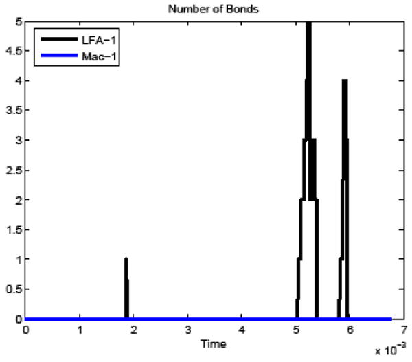
Time history of number of bonds formed between the white blood cell and cancer cell in the deformable PMN simulation.
Figure 11.
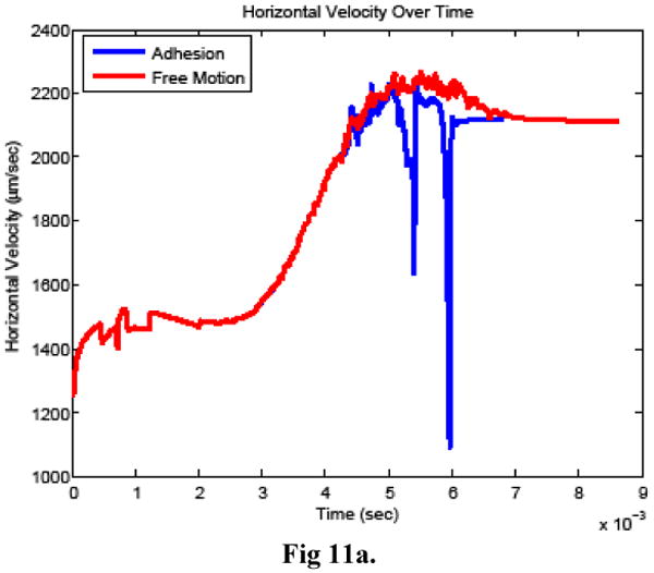
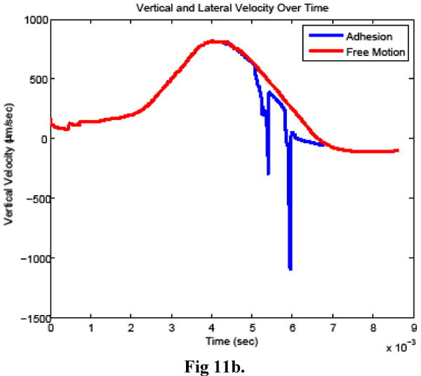
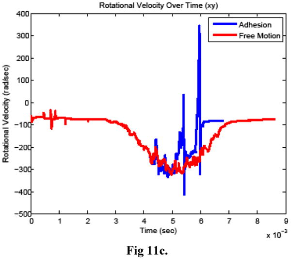
Cancer cell a) horizontal velocity, b) vertical velocity, and c) rotational velocity when bonds did (adhesion) and did not (free motion) form between the cells.
Figure 12 shows the simulation result at four time-steps including just before and after bonds formed between the two cells. The surface pressure on the white blood cell increases as the cancer cell moves toward it due to the bond formation. After the bonds break, the surface pressures decrease immediately (within 2 time steps or 1.6 μs) to the range seen before the bonds formed. The cancer cell then resumes its course at a similar velocity to that before the bonds formed, but remains closer to the white blood cell.
Figure 12.
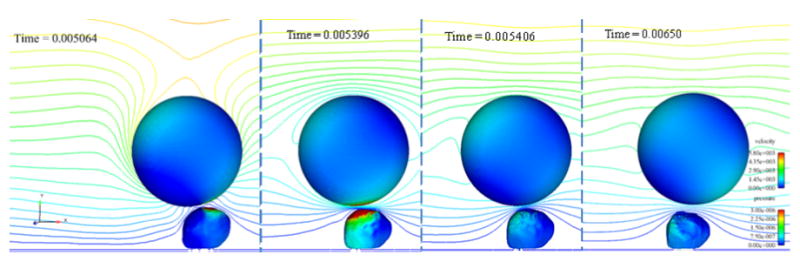
Four time steps of the collision simulation in which bonds formed between the cancer cell and white blood cell. Time steps shown are: a) before bonds form, b) when the number of bonds is a maximum, c) immediately after the bonds break, and d) one millisecond later. The cells are contoured by pressure (in kg/μm-s2) and a center clip plane is contoured by velocity magnitude (in μm/s). Flow direction is left to right.
5 Conclusions and future work
In this work, we have developed a quasi-steady technique to simulate low Reynolds number cellular interactions. The method involves coupling a succession of CFD, 6DOF, CSM, and surface biochemistry computations through a control script. The enabling component technologies used in the method are automatic adaptive grid generation (Harpoon), implicit pressure-velocity coupled CFD (AcuSolve), viscoelastic CSM (Abaqus), and modern biochemistry modeling of molecular bond formation and breakage.
The comparison between the forces applied to a cancer cell as it interacted with a white blood cell during transient and steady simulations verified the accuracy of the quasi-steady approximation. The cell-cell collision and interaction simulations presented demonstrated the coupling of the fluid-structure interaction, the biochemistry and the 6DOF capabilities.
Several simplifying assumptions were made in the model development. The assumptions that the cancer cell is rigid and interacts with a stationary PMN were based on experimental observations of the cells interacting in parallel plate flow chamber experiments (Liang, Slattery and Dong, 2005). It was assumed in this development work that the PMN deformation is due mainly to the fluid forces applied to it during the collision. A comparison of the fluid, adhesion, and repulsion forces on the PMN during the simulation presented here shows the adhesion and repulsion forces may also play a role in the local deformation of the PMN. This will be revisited in future work.
The PMN model included three components, an elastic membrane, a viscoelastic cytoplasm, and a rigid nucleus. The bulk and shear moduli were taken as constants in this work; inclusion of a full viscoelastic model is straightforward within the context of the method presented and is also nan area for future improvement.
As work continues, the authors are focused on the physics modeling improvements discussed above and computational optimization of the technique. The methodology is being used to study cancer cell interactions with white blood cells under physiologically relevant conditions.
Acknowledgments
The authors acknowledge and appreciate complimentary software licenses provided to the principal author by CEI, Inc. (Harpoon and Ensight) and ACUSIM Software, Inc. (AcuSolve) for her Ph.D. research, of which the present work is a component. The principal author was supported by an Educational and Foundational Research grant from the Pennsylvania State University Applied Research Laboratory. Support under NIH (NIH CA125707) and NSF (CBET-0729091) were also provided. Software assistance and discussions with Steve Cosgrove, Dave Corson, and Rob Campbell also benefitted this work.
Nomenclature
- A, AL
area contact area
- a, b
constants
- d
separation distance between rough cell surfaces
- ds
separation distance between smooth cell surfaces
- E
elastic modulus
- ed
deviatoric strain
- êi
unit vector
- ev
volumetric strain
- Fi
force vector
- G
shear modulus
- I
moment of inertia
- K
bulk modulus
- k
on- or off-rate for bond formation and breakage
- kb
Boltzmann's constant
- kon0, koff0
on- or off-rate under equilibrium conditions
- l
length dimension
- m
mass
- NR
number of random numbers generated
- nI
surface density of ICAM-1 molecules
- nˆi
normal vector
- nL
surface density of ligands
- nB
surface density of formed bonds
- P
probability of bond formation or breakage
- p
pressure
- R
cell radius
- Re
Reynolds number
- S
surface boundary
- s, sts
bond spring constant and transition state spring constant
- T
temperature
- t, tR
time, response time
- U
fluid velocity
- V
volume
- vi
velocity vector
- Wk
weight functions
- X
size parameter
- xi
coordinate vector
- δij
Kronecker delta
- δDij
virtual strain rate tensor
- εij
total elastic strain
- θi
rotation vector
- λ
equilibrium spring length
- μ
fluid viscosity
- ν
Poisson's ratio
- ρf
fluid density
- ρc
cell density
- σij
stress matrix
- τi
torque vector
- τij
stress tensor
- τm
time constant
Footnotes
Publisher's Disclaimer: This is a PDF file of an unedited manuscript that has been accepted for publication. As a service to our customers we are providing this early version of the manuscript. The manuscript will undergo copyediting, typesetting, and review of the resulting proof before it is published in its final citable form. Please note that during the production process errors may be discovered which could affect the content, and all legal disclaimers that apply to the journal pertain.
References
- ACUSIM Software Inc. http://www.acusim.com/html/acusolve.html.
- Bell GI. Models for the specific adhesion adhesion of cells to cells. Science. 1978;200:618–627. doi: 10.1126/science.347575. [DOI] [PubMed] [Google Scholar]
- Belk DM, Maple RC. Automated assembly of structured grids for moving body problems. AIAA Paper 1995-1680.Proceedings of the 12th AIAA Computational Fluid Dynamics Conference; 1995. [Google Scholar]
- Brennen CE. Cavitation and Bubble Dynamics. Oxford University Press; New York, NY: 1995. [Google Scholar]
- Bongrand P, Bell GI. Cell-Cell Adhesion: Parameters and Possible Mechanisms. Marcel Dekker Inc.; New York, NY: 1984. [Google Scholar]
- Bruehl RE, Springer TA, Bainton DF. Quantitation of L-selectin distribution on human leukocyte microvilli by immunogold labeling and electron microscopy. Journal of Histochemistry and Cytochemistry. 1996;44:835–844. doi: 10.1177/44.8.8756756. [DOI] [PubMed] [Google Scholar]
- Cao J, Donell B, Deaver DR, Lawrence MB, Dong C. In vitro side-view technique and analysis of human T-leukemic cell adhesion to ICAM-1 in shear flow. Microvascular Research. 1998;55:124–137. doi: 10.1006/mvre.1997.2064. [DOI] [PubMed] [Google Scholar]
- Cardoze D, Cunha A, Miller G, Phillips T, Walkington N. A bezier-based approach to unstructured moving meshes. Proceedings of the 20th Annual Symposium on Computational Geometry. 2004 ACM Paper 1-58113-885-7. [Google Scholar]
- Ronald Darby. Viscoelastic Fluids: An Introduction to their Properties and Behavior. Marcel Dekker, Inc.; New York, NY: 1976. [Google Scholar]
- Dembo M, Torney D, Saxaman K, Hammer D. The reaction-limited kinetics of membrane-to-surface adhesion and detachment. Proceedings of the Royal Society of London B Biology. 1988;234:55–83. doi: 10.1098/rspb.1988.0038. [DOI] [PubMed] [Google Scholar]
- De Zeeuw D, Powell KG. An adaptively refined Cartesian mesh solver for the Euler equations. Journal of Computational Physics. 1993;104:56–68. [Google Scholar]
- Dong C, Lei XX. Biomechanics of cell rolling: Shear flow, cell-surface adhesion, and cell deformability. Journal of Biomechanics. 2000;33:35–43. doi: 10.1016/s0021-9290(99)00174-8. [DOI] [PubMed] [Google Scholar]
- Dong C, Skalak R, Paul KL, Sung P, Schmid-Schonbein G, Chien S. Passive deformation analysis of human leukocytes. Journal of Biomechanical Engineering. 1988;110:27–36. doi: 10.1115/1.3108402. [DOI] [PubMed] [Google Scholar]
- Dong C, Skalak R. Leukocyte deformability: Finite element modeling of large viscoelastic deformation. Journal of Theoretical Biology. 1992;158:173–193. doi: 10.1016/s0022-5193(05)80716-7. [DOI] [PubMed] [Google Scholar]
- Dong C, Skalak R, Sung KLP. Cytoplasmic rheology of passive neutrophils. Biorheology. 1991;28:557–567. doi: 10.3233/bir-1991-28607. [DOI] [PubMed] [Google Scholar]
- Dong C, Cao J, Struble E, Lipowsky HH. Mechanics of leukocyte deformation and adhesion to endothelium in shear flow. Annals of Biomedical Engineering. 1999;27:298–312. doi: 10.1114/1.143. [DOI] [PubMed] [Google Scholar]
- Dong C, Slattery MJ, Liang S. Micromechanics of tumor cell adhesion and migration under dynamic flow conditions. Frontiers in Bioscience. 2005;10:379–384. doi: 10.2741/1535. [DOI] [PMC free article] [PubMed] [Google Scholar]
- Freitas CJ, Runnels SR. Simulation of Fluid-Structure Interaction Using Patched-Overset Grids. Journal of Fluids and Structures. 1999;13:191–207. [Google Scholar]
- Hammer D, Apte S. Simulation of cell rolling and adhesion on surfaces in shear flow: general results and analysis of selectin-mediated neutrophil adhesion. Biophysical Journal. 1992;62:35–57. doi: 10.1016/S0006-3495(92)81577-1. [DOI] [PMC free article] [PubMed] [Google Scholar]
- Hirt C, Nichols B. Volume of fluid (VOF) method for the dynamics of free Boundaries. Journal of Computational Physics. 1981;39:201–225. [Google Scholar]
- House S, Lipowsky H. In vivo determination of the force of leukocyte endothelium adhesion in the mesenteric microvasculature of the cat. Circulatory Research. 1988;63:658–668. doi: 10.1161/01.res.63.3.658. [DOI] [PubMed] [Google Scholar]
- Hoskins MH, Dong C. Kinetics analysis of binding between melanoma cells and neutrophils. Molecular Cell Biomechanics. 2006;3(2):79–87. [PMC free article] [PubMed] [Google Scholar]
- Hu HH, Patankar N, Zhu M. Direct numerical simulations of fluid-solid systems using the arbitrary Lagrangian-Eulerian technique. Journal of Computational Physics. 2001;169:427–462. [Google Scholar]
- Jansen KE, Collis SS, Whiting C, Shakib F. A better consistency for low order stabilized finite element methods. Computer Methods in Applied Mechanics and Engineering. 1999;174(1):153–170. [Google Scholar]
- Johnson K, Bittorf KJ. Validating the Galerkin least-square finite element methods in predicting mixing flows in stirred tank reactors. Proceedings of the 10th Annual Conference of the CFD Society of Canada.2002. [Google Scholar]
- Kan HC, Udaykumar H, Shyy W, Tran-Son-Tay R. Hydrodynamics of a compound drop with application to leukocyte modeling. Physics of Fluids. 1998;10:760–774. [Google Scholar]
- Khismatullin DB, Truskey GA. Three-dimensional numerical simulation of receptor-mediated leukocyte adhesion to surfaces: Effects of cell deformability and viscoelasticity. Physics of Fluids. 2005;17:1–20. 031505. [Google Scholar]
- King MR, Hammer DA. Multiparticle adhesive dynamics: Interactions between stably rolling cells. Biophysical Journal. 2001;81(26):799–813. doi: 10.1016/S0006-3495(01)75742-6. [DOI] [PMC free article] [PubMed] [Google Scholar]
- Kunz RF, Yu WS, Antal SP, Ettorre SM. An unstructured two fluid method based on the coupled phasic exchange algorithm. AIAA Paper; AIAA Computational Fluid Dynamics Conference; 2001. pp. 2001–2672. [Google Scholar]
- Lei X, Lawrence MB, Dong C. Influence of cell deformation on leukocyte rolling adhesion in shear flow. Journal of Biomechanical Engineering. 1999;121:636–643. doi: 10.1115/1.2800866. [DOI] [PubMed] [Google Scholar]
- Leroyer A, Visonneau M. Numerical Methods for RANSE Simulations of a Self-Propelled Fish-Like Body. Journal of Fluids and Structures. 2005;20:975–991. [Google Scholar]
- Leyton-Mange J, Yang S, Hoskins MH, Kunz RF, Zahn JD, Dong C. Design of a side-view particle imaging velocimetry flow system for cell-substrate adhesion studies. Journal of Biomechanical Engineering. 2006;128:271–278. doi: 10.1115/1.2165689. [DOI] [PMC free article] [PubMed] [Google Scholar]
- Liang S, Slattery M, Dong C. Shear stress and shear rate differentially affect the multi-step process of leukocyte-facilitated melanoma adhesion. Experimental Cell Research. 2005;310:282–292. doi: 10.1016/j.yexcr.2005.07.028. [DOI] [PMC free article] [PubMed] [Google Scholar]
- Liu WK, Liu Y, Farrell D, Zhang L, Wang XS, Fukui Y, Patankar N, Zhang Y, Bajaj C, Lee J, Hong J, Chen X, Hsu H. Immersed finite element method and its application to biological systems. Computer Methods in Applied Mechanics and Engineering. 2006;195:1722–1749. doi: 10.1016/j.cma.2005.05.049. [DOI] [PMC free article] [PubMed] [Google Scholar]
- Migliorini C, Qian Y, Chen H, Brown EB, Jain RK, Munn LL. Red blood cells augment leukocyte rolling in a virtual blood vessel. Biophysical Journal. 2002;83:1834–1841. doi: 10.1016/S0006-3495(02)73948-9. [DOI] [PMC free article] [PubMed] [Google Scholar]
- Mittal R, Iaccarino G. Immersed boundary methods. Annual Review of Fluid Mechanics. 2005;37:239–261. [Google Scholar]
- Mulholland JW, Shelton JC, Luo XY. Blood Flow and Damage by the Roller Pumps During Cardiopulmonary Bypass. Journal of Fluids and Structures. 2005;20:129–140. [Google Scholar]
- N'Dri N, Shyy W, Tran-Son-Tay R. Computational modeling of cell adhesion and movement using a continuum-kinetics approach. Biophysical Journal. 2003;85:2273–2286. doi: 10.1016/s0006-3495(03)74652-9. [DOI] [PMC free article] [PubMed] [Google Scholar]
- Noack R. SUGGAR: A general capability for moving body overset grid assembly. AIAA Paper 2005-5117.Proceedings of the 17th Annual AIAA Computational Fluid Dynamics Conference; 2005. [Google Scholar]
- Noack R. DiRTlib: A Library to Add an Overset Capability to Your Flow Solver. AIAA Paper 2005-5116.Proceedings of the 17th Annual AIAA Computational Fluid Dynamics Conference; 2005. [Google Scholar]
- Osher S, Fedkiw R. Level Set Methods and Dynamic Implicit Surfaces. Springer-Verlag New York, Inc; 2003. [Google Scholar]
- Osher S, Sethian J. Fronts propagating with curvature dependent speed: Algorithms based on Hamilton-Jacobi formulations. Journal of Computational Physics. 1988;79:12–49. [Google Scholar]
- Peskin CS. The immersed boundary method. Acta Numerica. 2002;11:479–517. [Google Scholar]
- Pivkin IV, Richardson PD, Karniadakis G. Blood flow velocity effects and role of activation delay time on growth and form of platelet thrombi. Proceedings of the National Academy of Sciences. 2006;103(46):17164–17169. doi: 10.1073/pnas.0608546103. [DOI] [PMC free article] [PubMed] [Google Scholar]
- Slattery MJ, Liang S, Dong C. Distinct role of hydrodynamic shear in leukocyte-facilitated tumor cell extravasation. American Journal of Physiology; Cell Physiology. 2005;288:C831–C839. doi: 10.1152/ajpcell.00439.2004. [DOI] [PMC free article] [PubMed] [Google Scholar]
- Sharc Ltd. http://www.sharc.co.uk/index.htm.
- Shyy W, Francois M, Udaykumar H, N'Dri N, Tran-Son-Tay R. Moving boundaries in micro-scale biofluid dynamics. Applied Mechanics Reviews. 2001;54:405–452. [Google Scholar]
- Simon SI, Green CE. Molecular mechanics and dynamics of leukocyte recruitment during inflammation. Annual Review of Biomedical Engineering. 2005;7:151–185. doi: 10.1146/annurev.bioeng.7.060804.100423. [DOI] [PubMed] [Google Scholar]
- Simulia http://www.simulia.com/products/abaqus_standard.html.
- Togashi F, Ito Y, Nakahashi K, Obayashi S. Overset unstructured grids method for viscous flow computations. Proceedings of the 21st AIAA Applied Aerodynamics Conference; 2003. AIAA Paper 2003-3405. [Google Scholar]
- Zhang L, Gerstenberger A, Wang X, Liu WK. Immersed finite element method. Computer Methods in Applied Mechanics and Engineering. 2004;193:2051–2067. [Google Scholar]