Segmented transition pathway of the signaling protein nitrogen regulatory protein C

Abstract

Recent advances in experimental methods are providing increasing evidence that proteins sample conformational substates important for function in the absence of their ligands. An example is the receiver domain of nitrogen regulatory protein C (NtrC^R), a member of the phosphorylation-mediated signaling family of “two-component systems”. NtrC^R samples both the inactive and active conformation before phosphorylation. Here we determine a possible pathway of interconversion between the active and inactive state by targeted molecular dynamics (TMD) simulations and quasi-harmonic analysis; these methods are used because the experimental conversion rate is in the μs range, longer than that easily accessible to atomistic molecular dynamics (MD) simulations. The calculated pathway is found to be composed of four consecutive stages described by different progress variables. The lowest quasi-harmonic principal components from unbiased MD simulations on the active state correspond to the first stage, but not the subsequent stages of the transition. The TMD pathway suggests that several transient non-native hydrogen bonds may facilitate the transition.

Introduction

The ability of many proteins to undergo well-defined conformational changes is a key element in their function. The different conformations that are sampled during activity are present in varying amounts, depending on the absence or presence of ligands that stabilize one conformational state, relative to another [1, 2, 3, 4, 5, 6, 7, 8]. As the number of proteins for which conformational substates are known is increasing, the question of how folded proteins can interconvert efficiently among theses folded substates is gaining interest. Since the details of the pathways followed in the conformational transitions are not easily accessible by experiment, computation studies play an important role in providing complementary information. Typically the time scale (high μs to ms in most systems) of the transition is too long for direct observation in full atomic molecular dynamics (MD) simulations, though there are exceptions in which the conformational change is fast enough to observe on the nanosecond timescale [9, 10]. Consequently, the development of methods for calculating possible pathways and the free energy barriers involved is a very active field of research. There is a vast and still rapidly growing literature on this subject of which we list only some representative papers [11, 12, 13, 14, 15, 16, 17, 18, 19, 20, 21]. In the present paper, we apply two of these methods (targeted molecular dynamics, TMD [11, 14, 22] and quasi-harmonic analysis [23, 24, 25] to study the conformational transition between the inactive and active form of a bacterial signaling protein, the receiver domain of the nitrogen regulatory protein C (NtrC^R). The essential point of both methods is to use simulations on the ns time scale to obtain information about much slower events. Applications have shown that meaningful results can be obtained in this way [26, 27, 28, 29, 30, 31].

NtrC^R belongs to the family of “two-component systems” that are the key signaling modules in bacteria [32]. The three-dimensional structures of the inactive and active state conformations have been solved by NMR [33, 34, 35, 36] (Figure 1). Both conformations, the inactive and active state, are populated at room temperature, with the population of the active conformation considerably smaller (14% at 300K) than that of the inactive one in the unphosphorylated form, while after phosphorylation the active form dominates (more than 99%) [35, 37]. The rate of interconversion in unphosphorylated NtrC^R was measured by NMR relaxation methods to be about 13,000/s [37].

Figure 1.

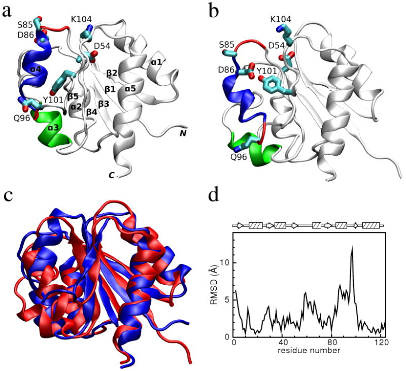
Comparison of the inactive and active conformations of NtrC^R (modified from Figure 3 of Kern et al. [33]). The inactive (PDB 1DC7)(a) and the active (PDB 1DC8)(b) conformations of NtrC^R [33] are shown highlighting the elements involved in the proposed transition pathway: backbone of the α3-helix (green) and α4-helix (blue), backbone of residues at the N- and C-termini of the α4-helix (His84, Ser85, Gln95 and Gln96), the side chains of Asp54, Ser85, Asp86, Gln96, Tyr101 and Lys104 rendered as thick sticks and colored by atom types: Carbon, nitrogen and oxygen atoms are cyan, blue and red respectively. Superposition of the inactive (blue) and active (red) conformations (c) and backbone root mean square deviation (RMSD) between the two conformations as a function of residue number (d).

The fact that the high resolution structures of the end states and the rate of interconversion are known from experiments and that both conformations are sampled at room temperature in the absence of phosphorylation makes NtrC^R an excellent model system for the use of computational methods to study the transition pathway. We apply TMD to find the transition path between the active and inactive form. An analysis of the resulting trajectory shows that there are four distinct stages, each of which is best represented by one or two different progress variables. Additional TMD trajectories confirmed this analysis. In addition, several non-native hydrogen bonds are observed that transiently exist but are absent in the end state structures. A comparison with the principal components from a quasi-harmonic analysis of the active structure shows that low frequency principal components overlap better with the first stage of the transition than with the remainder of the transition. The present study provides new insights into the nature of this complex transition. It also resolves certain questions raised in previous work [38, 39, 40]. We consider these papers in the Discussion section. Of particular interest is that we find no evidence for “cracking” (local unfolding), which has been suggested to be an essential element of the conformational transition [39].

Results

MD Simulation and quasi-harmonic analysis

The original NMR structures of NtrC^R [33] are first refined by MD simulations in the presence of experimental NOE distance constraints. The refinement protocol follows examples in the literature [41, 42, 43, 44, 45, 46, 47], with the main difference that we simulate the system for one nanosecond, while most simulations in the literature were limited to tens or hundreds of picoseconds. Details are given in the Methods section. WHATIF Z-scores [48], which are often used to estimate the geometric quality of structures, are improved to acceptable ranges by the refinement procedure (Table 1). The refinement procedure also improves the agreement between chemical shifts computed by the SPARTA program [49] and the experimental data (Table 2). Since chemical shift predictions are sensitive to local geometrical properties such as hydrogen bonds and backbone torsion angles, the improved agreement between predicted and experimental chemical shifts is a direct indication of the improvements in the structure. Most importantly, the backbone hydrogen bonds are improved by the refinement procedure. The total number of backbone hydrogen bonds, detected by the secondary structure prediction program DSSP [50], is increased from 72 to 87 for the inactive state, and from 60 to 75 for the active state. In the α4-helix whose conformational transition is of primary interest, the number of regular helical backbone hydrogen bonds is increased from 3 to 6 in the inactive state, and from 2 to 6 in the active state. The number of 3₁₀-helical or π-helical hydrogen bonds is reduced from 1 to none in the inactive state, and from 4 to 2 in the active state. The backbone hydrogen bonds are important for the stability of secondary structure. In fact, comparison simulations with the unrefined NMR structure showed unfolding of the α4-helix (data not shown).

Table 1.

WHATIF [48] Z-scores.

	inac-NMR	inac-ref	acti-NMR	acti-ref
Ramachandran plot	-6.82	2.48	-7.28	1.30
χ1/χ2 correlation	-7.16	-1.39	-6.99	-2.00
packing	-2.20	0.67	-2.45	-0.36
backbone conformation	-6.91	-1.00	-8.04	-1.46

WHATIF [48] Z-scores of the secondary structures of the original NMR structures and of the refined structures. Inac-NMR and acti-NMR are the NMR structures [33] of the inactive and active states respectively, while inac-ref and acti-ref are the corresponding structures structures after refinement with the simulations. The Z-scores that are considered to be low by WHATIF (outside of ±4) are marked in bold.

Table 2.

Correlation between computed and experimental chemical shifts.

	inac-NMR	inac-ref	acti-NMR	acti-ref
H	0.27	0.55	0.34	0.42
Hα	0.73	0.84	0.75	0.82
N	0.72	0.84	0.75	0.81
Cα	0.94	0.96	0.93	0.95

Linear correlation coefficients between chemical shifts computed by the SPARTA program [49] based on the original and the refined structures and measured by NMR experiments [33]. Inac-NMR and acti-NMR are the NMR structures [33] of the inactive and active states respectively, while inac-ref and acti-ref are the corresponding structures after refinement with the simulations. For reference, the linear correlation coefficients between the predicted and experimental chemical shifts are 0.79 for backbone nitrogen (N), 0.69 for backbone amide hydrogen (H), 0.85 for α-hydrogen (Hα), and 0.91 for backbone α-carbon (Cα) for a library of proteins [49].

To investigate the flexibility of the inactive and active conformations on the nanosecond time scale, the refined inactive and active structures are simulated for 15ns each in explicit solvent using the CHARMM force field [51], which was employed in the refinement. Since the root mean square deviation (RMSD) time traces reach a plateau after 3ns (Figure 2), the 3ns to 15ns segments of the two simulation trajectories are considered as equilibrated and used for analysis. The backbone root mean square fluctuation (RMSF) of the equilibrated segments of the two simulation trajectories show that those of the inactive stricture are larger than for the active one; this is in agreement with earlier work of Hu et al. [38]. Moreover, the RMSF values are larger where the two structures differ most (Arg56 to Gln71 and Gln95 to Phe99), particularly in the inactive state (Figure 2).

Figure 2.

(a) The time traces of the backbone root mean square deviation (RMSD) from the refined NMR structures for the trajectories: inactive in blue and active in red. (b) The backbone root mean square fluctuation (RMSF) of the simulation trajectories using the refined inactive (blue) and the refined active (red) conformations. The 3ns to 15ns segments of the 15ns simulation trajectories are used in the computation of RMSF.

To determine the larger scale concerted motion directions in the two end states, quasi-harmonic analysis (QHA) [23, 24, 25] are performed on the equilibrated segments of the simulation trajectories. In QHA, the protein dynamics in the 3N Cartesian space is projected onto 3N orthonormal motion directions, which are termed quasi-harmonic principal components (QHPCs or PCs). With increasing index, each PC describes a motion direction of decreasing fluctuation amplitude. Hence the first PC is the motion direction with the largest fluctuation amplitude; the second PC is the motion direction with the second largest fluctuation amplitude, etc. The low indexed PCs are the most likely motion directions. QHA of domain structured proteins have shown that the first several PCs often correlate well with the large scale conformational transitions in these proteins [52, 53, 54].

The involvement coefficient indicates the amount of overlap between a PC and a probe direction. It is the absolute value of the dot product between the unit vector of a PC and the unit vector of a probe direction (see Methods). When the probe direction is the structural difference between two end states, the involvement coefficient describes how much the motion direction of a PC overlaps with the conformational difference between two end states. In the domain structured protein adenylate kinase (AdK), the involvement coefficients of the first two PCs are 0.49 and 0.63 respectively, whereas those of the other PCs are at least several folds smaller [53]. In NtrC^R, by contrast, the involvement coefficients of all PCs are small and rather uniformly distributed (Figure 3a,b). Thus the first several PCs of both end states of NtrC^R do not point directly to the other state. The cumulative involvement coefficient (see Methods) quantifies the percentage of the conformational difference accounted for by the sub-space of low indexed PCs. In NtrC^R, the cumulative involvement coefficient of the first 50 PCs is merely 0.36 and 0.30 for the inactive and active states, respectively (Figure 3a,b). In other words, the majority of the conformational difference between the two end states of NtrC^R is not covered by the first 50 PCs of either end state. As a comparison, in the protein AdK, the cumulative involvement coefficient of the first five PCs is 0.82 [53]. In other words, more than 80% of the conformational difference between the open and the closed states of AdK take place within a five-dimensional space composed by the five lowest indexed PCs.

Figure 3.

The involvement coefficients (thin bars, left y-axis) and the cumulative involvement coefficients (thick line, right y-axis) of the first 50 quasi-harmonic principal components. The involvement coefficients are calculated by projecting the principal components of the MD simulation of the inactive conformation (a) and of the active conformation (b) onto the vector connecting the active and inactive structures (see text for definitions). In (c), the principal components of the active state are projected onto the motion direction of the first segment of the transition (see text).

Since the low indexed PCs do not overlap much with the structural difference between the end states, the transition pathway between the initial and the target states likely involve higher indexed PCs. For this reason, those coarse grained algorithms that build pathways by extrapolating low indexed PCs are not suitable for studying the detailed transition events of NtrC^R. We anticipate that only a detailed all-atom algorithm coupled with a sophisticated force field is capable of generating reasonable pathways between the two end states of NtrC^R.

Segmented Transition Pathway

There are four major conformational differences at the α4-helix between the inactive and the active states (Figure 1). First, the orientation of the α4-helix relative to the β-strands is different in the two conformations. Second, the α4-helix rotates so that its hydrophobic residues of Leu87, Ala90 and Val91 are exposed to solvent in the active state while they are buried in the inactive state [33]. Third, the registry of the α4-helix is different in the two conformations. The α4-helix is composed of residues from His84 to Tyr94 in the inactive state, while from Asp86 to Gln96 in the active state. Fourth, the α4-β5 loop flips, facing the α5-helix in the inactive state and the α3-helix in the active state. The goal is to investigate the pathway by which this complicated rearrangement occurs.

A transition pathway is constructed by the TMD algorithm. The length of the TMD simulation is 3.5ns, during which the all heavy atom RMSD between the initial and the target structures is forced to be reduced from 3.8Å to 0.3Å. The residue Asp54 is not phosphorylated in either end state structure. This is justified by the experimental evidences that both the inactive and the active state structures are populated when Asp54 is not phosphorylated [35, 37]. Since the free energy of the active state is higher than that of the inactive state in non-phosphorylated NtrC^R [35, 37], the free energy barrier is lower in going from the active to the inactive state than in the opposite direction. The lower the free energy barrier, the smaller the magnitude of the biasing potential that is required in the TMD calculation. Consequently, the trajectory is calculated from the active to the inactive state. We want to point out again that biasing potentials must be used in order to compute this pathway since the experimentally observed rates of interconversion are in the high μs range [37], significantly beyond the time accessible to all-atom molecular dynamics simulations except with very large supercomputers or special hardware.

The computed transition pathway is complex. As we have seen, the overall pathway is not along the direction of a few low indexed PCs. In accord with this result, there does not appear to be a single generalized progress variable (“reaction coordinate”) to represent the entire pathway. The complexity results from the rather intricate structural difference between the two end states. A careful inspection of the calculated TMD pathway reveals that it could be dissected into four main consecutive stages, each of which corresponds to a transition which is represented by one- or two-dimensional progress variables. The characteristic motions and progress variables of the four transition stages of the α4-helix are summarized in Figure 4; see also the animation in the supplementary material. The details of the four stages are described below.

Figure 4.

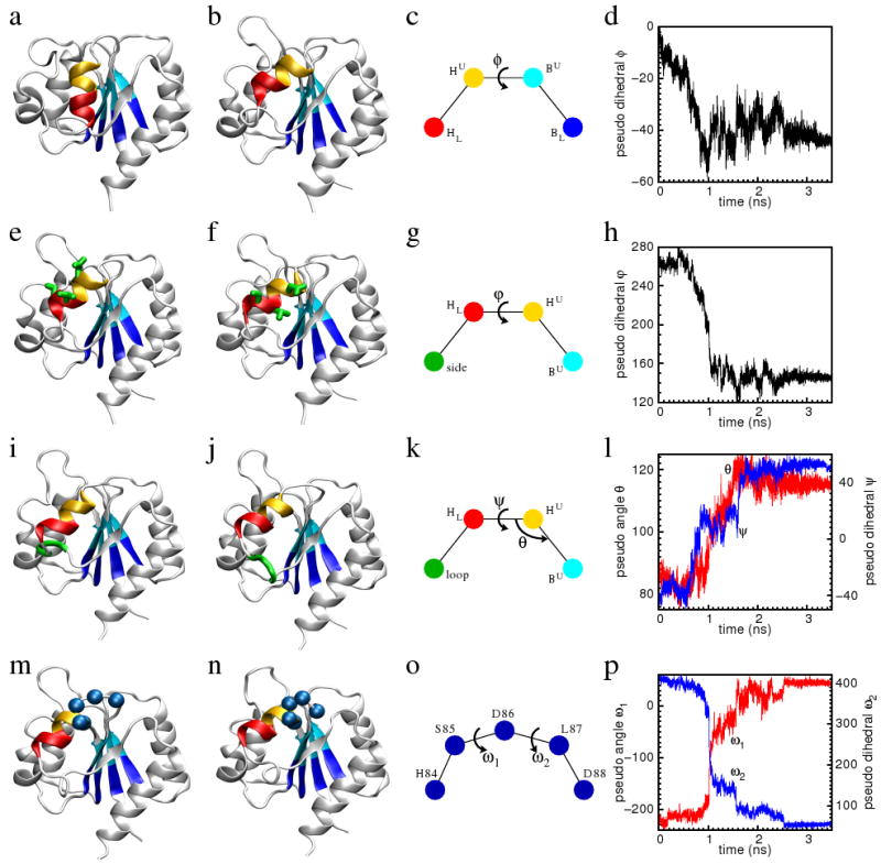
The characteristic motions and reaction coordinates of the tilt (the first row), the rotation (the second row), the flip (the third row), and the adjust (the fourth row) stages of the transition. In each row, the first two sub-figures are the conformations before and after the transition. The third sub-figure illustrates the reaction coordinates of the transition. The colored spheres represent the center of masses (CM) of the residues of the same color shown in the first two sub-figures of the same row. The reaction coordinates are designated by Greek letters. The fourth sub-figure shows the time traces of the reaction coordinates along the whole TMD trajectory. The residues in the lower half of the first four β-stands (residues Val6, Trp7, Cys30, Thr31, Val50, Leu51, Val78 and Ile79) are colored blue. Their CM is designated as B_L. The residues in the upper half of the first four β-stands (residues Val8, Val9, Thr32, Phe33, Leu52, Ser53, Ile80 and Met81) are colored cyan. Their CM is designated as B^U. The residues in the upper half of the α4-helix (residues Leu87, Asp88, Ala89, and Ala90) are colored orange. Their CM is designated as H^U. The residues in the lower half of the α4-helix (residues Val91, Ser92, Ala93, and Tyr94) are colored red. Their CM is designated as H_L. In Figure (e) and (f), residues Asp88, Val91 and Ser92 are rendered by thick sticks and colored green. Their CM is designated as side. In Figure (i) and (j), the three residues Gln96, Gly97 and Ala98 are rendered as thick ribbon and colored green. Their CM is designated as loop. In Figure (m) and (n), the Cα-atoms of residues His84, Ser85, Asp86, Leu87 and Asp88 are rendered as spheres and colored blue.

First stage: tilt of the α4-helix

During the first 0.85ns of the whole 3.5ns TMD trajectory, the axis of the α4-helix tilts so that its C-terminus moves toward the α3-helix. The N-terminus of the α4-helix has little displacement because the N-terminus is connected to the stable β4-strand by a short turn of three residues. The transition in this stage can be quantified by the pseudo dihedral-angle defined in term of the four pseudo atoms B_L–B^U–H^U–H_L, as illustrated in Figure 4c.

The α4-helix loses two C-terminal residues at the end of the tilt stage of the transition. In the active state structure, the residues of Gln95 and Gln96 are at the C-terminus of the helix. The main chain i → i + 4 hydrogen bonds between Gln95 and Val91, and Gln96 and Ser92 are distorted then broken when the C-terminus of the α4-helix moves toward the α3-helix. Gln95 and Gln96 subsequently form hydrogen bonds with solvent and the main chain carbonyl oxygen of Ala93, respectively. His84 and Ser85 are still in the β4-α4 loop. Therefore the registry shift transition of the α4-helix is not complete at the end of the tilt stage of the transition. Though the α4-helix has lost two C-terminus residues, it has not yet recruited His84 and Ser85 to the α4-helix at its N-terminal end.

Second stage: axial rotation of the α4-helix

During 0.65 ns to 1.06 ns, somewhat displaced during the first transition stage, the α4-helix rotates around its own axis by about 110°. The transition in this stage can be quantified by a pseudo-dihedral formed by four pseudo atoms B^U–H^U–H_L–side, which changes from 260° to 150° (Figure 4g). The three residues of Asp88, Val91 and Ser92 are at one side of the α4-helix, and as a consequence of the rigid body rotation of the α4-helix, their orientation is changed (Figure 4e,f). The overall effect of the rotation transition is to bury two hydrophobic residues Leu87 and Ala90, while the hydrophobic residue Ala89 is exposed after this transition. The polar residue Ser92, which faces the protein interior in the active state structure, becomes exposed to solvent. Both Asp88 and Val91 remain exposed, though their orientations relative to the rest of the protein are changed.

Third stage: flip transition

During 1.06 ns to 1.65 ns of the TMD trajectory, the C-terminus of the α4-helix moves further away from the β-strands, followed by the flip of the α4-β5 loop from facing the α3-helix to facing the α5-helix (Figure 4i,j). The transition in this stage can be quantified by two progress variables. One is the pseudo angle between the pseudo atoms B^U–H^U–H_L. This pseudo angle quantifies the separation of the C-terminus of the α4-helix from the β-strands. The other progress variable is the pseudo dihedral formed by four pseudo atoms of B^U–H^U–H_L–loop (Figure 4k). This pseudo-dihedral angle increases at the end of the tilt stage of the transition, when Gln95 and Gln96 separate from the C-terminus of the α4-helix (Figure 4l). It is stable at around 0° for a short duration when the α4-β5 loop faces the α3-helix. During 1.6ns to 1.65ns, this pseudo dihedral angle increases sharply to about 50° when the α4-β5 loop moves to the opposite side of the α4-helix.

Fourth stage: adjust transition

The conformational transition is almost complete after the first three stages. At this point His84 and Ser85 have moved spatially close to Asp88 and Ala89. During the fourth stage, His84 and Ser85 form stable i → i + 4 main chain hydrogen bonds with Asp88 and Ala89, respectively. Consequently, His84 and Ser85 become the N-terminal residues of the α4-helix, and the α4-helix gains half a helical turn. The registry shift in the α4-helix is now complete.

The pseudo-dihedral angles formed by four consecutive Cα-atoms between His84 and Leu87 and between Ser85 and Asp88 are two progress variables that quantify the unification of His84 and Ser85 into the α4-helix (Figure 4o). Up to about 1ns, both pseudo-dihedral angles remain near their initial values. They then undergo a transition during which they fluctuate (1 to 2.5ns). After the transition, when the main chain hydrogen bonds form between His84 and Asp88 as well as between Ser85 and Ala89, both pseudo-dihedral angles are stabilized at about 50° (Figure 4p).

Restrained simulation along the proposed progress variables

To demonstrate that the progress variables introduced above are sufficient to quantify the conformational transition in NtrC^R, we run a simulation starting with the active state structure and apply restraint potentials sequentially along these variables; details of the simulations are given in Methods.

A 16ns simulation is run starting from the refined active structure. In the first 4ns, a restraint potential is applied so that the proposed progress variable of the tilt stage of the transition fluctuates around its value in the refined inactive state structure. In the second 4ns segment, in addition to the one used in the first 4ns segment, a restraint potential is applied so that the proposed progress variable of the rotation stage of the transition fluctuates around its value in the refined inactive structure. In the third 4ns segment, two additional restraint potentials are applied to introduce the flip stage of the transition. During the final 4ns segment, two restraint potentials are added along the proposed progress variables of the adjust stage of the transition. The protein is found to transform gradually and in a segmented way from the active conformation to the inactive conformation; the final snapshot of the restrained simulation is within the range of the RMSD fluctuations shown in the unbiased MD simulation of the refined inactive structure. As shown in Figure 5, after the restrained simulation, the relative position and orientation of the α4-helix with respect to the β-strands look very similar to those in the refined inactive structure. These results support the conclusion that the six progress variables proposed in this paper are sufficient to describe the conformational transitions in NtrC^R.

Figure 5.

Comparison of the refined active state structure (a), the final snapshot of the simulation on the active state structure with restrained potentials applied along the six proposed progress variables (b), and the refined inactive state structure (c). The backbones of the following residues are colored: the α4-helix (Asp86 to Tyr94) in orange; His84 and Ser85 in blue; Gln95 to Ala98 in purple. The side chains of Asp88, Val91 and Ser92 are rendered by thick green sticks.

Principal components projected on the first stage of the transition

As described above, the direction of the motion corresponding to low frequency PCs of NtrC^R do not correlate with the conformational difference between the two end states of NtrC^R. Since the low frequency PCs correspond to the large amplitude motion directions exhibited in the 12ns (3ns to 15ns) MD simulations, while the conformational transition is in the high μs to ms time range [37], this lack of correlation may not be surprising. However, it should be noted that in some other cases of slow conformational changes, particular for hinge motions, the PCA results do correspond to the transition [28, 53, 55]. The lack of correlation between the dynamics on different time scales found for NtrC^R results from the segmented nature of the transition pathway, in which the first stage of the conformational transition from the active state does not point directly at the inactive state. Rather, it leads to an intermediate conformation that has not been detected experimentally. The snapshot at the end of the 4ns simulation with a restraining potential on the proposed progress variable of the first stage of the transition, is taken as a model of the intermediate conformation. When the first 50 PCs of the active state are projected along the structural difference between the refined active structure and the modeled intermediate structure, their cumulative involvement coefficient is equal to 74.4% (Figure 3c). Hence the direction of the motion of the low frequency PCs correlate well with the first stage of the conformational transition. In other words, the ps to ns dynamics of NtrC^R in its active state is largely along the initial segment of the transition pathway between the active and the inactive state. This is in accord with the normal mode study of rasp21 [14]; see also Yang et al. [56] for a related discussion.

Transient hydrogen bonds

To identify the critical hydrogen bonds that may assist the conformational transition in NtrC^R, we have analyzed the appearance and disappearance of hydrogen bonds along the 3.5ns TMD trajectory. By using a hydrogen to acceptor cut-off distance of 2.5Å and a donor–hydrogen–acceptor cut-off angle of 120°, we identify a total of 466 hydrogen bonds that are present in at least one of the 3500 snapshots saved along the simulated pathway. Four of these satisfy the following three criteria: (i) they are not present in either end state structures but are present in more than 50 consecutive snapshots along the transition pathway; (ii) they are spatially close to the α3- and the α4-helices, where the conformational transition takes place; (iii) either the donor or the acceptor is a side chain atom. These four hydrogen bonds are between Ser85 and Asp86, between Ala90 and Gln96, between Ala93 and Gln96, and between Gln96 and Tyr101 (Figure 6).

Figure 6.

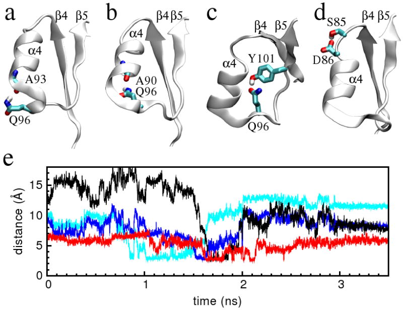
Transient hydrogen bonds that are present during the transition trajectory and absent in both the inactive and the active state structures. Snapshots of the hydrogen bonds between Gln96 and Ala93 (a), between Gln96 and Ala90 (b), between Gln96 and Tyr101 (c), and between Ser85 and Asp86 (d) are shown. (e) Time traces of the distance between the Gln96 Nε atom and the Ala93 carbonyl oxygen atom (cyan), between the Gln96 Nε atom and the Ala93 carbonyl oxygen atom (blue), between the Gln96 Oε atom and the Tyr101 Oη atom (black), and of the minimum distance between the Ser85 Oγ atom and the Asp86 Oδ atoms (red) are shown.

The side chain of Gln96 forms a transient hydrogen bond relay network with Ala93, Ala90 and Tyr101 (Figure 6). At the C-terminus of the α4-helix, the Gln96 side chain Hε atoms and the Ala93 carbonyl oxygen atom form a hydrogen bond during the 1.0ns to 1.5ns segment of the trajectory. This time range overlaps with the late stage of the axial rotation of the α4-helix. At about 1.5ns, the Gln96 side chain Hε atoms dissociate from Ala93 and form hydrogen bonds with the Ala90 carbonyl oxygen atom. Shortly thereafter between 1.6ns to 1.8ns, the Gln96 side chain Oε1 atom and the Tyr101 side chain Hη atom form a temporary hydrogen bond. Almost in the same time period (1.6–2.1ns), a hydrogen bond is formed between the Ser85 side chain Hγ and the Asp86 side chain Oδ atoms (Figure 6). This time range roughly coincides with the flip transition of the α4-β5 loop, which takes place at the C-terminal end of the α4-helix. Hence, a hydrogen bond in the vicinity of the C-terminal end of the α4-helix (that between Gln96 and Tyr101) may facilitate the transition. The fact that a hydrogen bond at the N-terminal end of the α4-helix (between Ser85 and Asp86) forms and breaks at the same time, hints at a collective nature of the conformational transition.

Three solvent bridged transient hydrogen bonds are also present during the transition. Water mediated hydrogen bonds between the His84:Hδ1 atom and the Asp86:Oδ atoms, between the His84:HN atom and the Tyr101:Oη atom, and between the Tyr101:Oη atom and the Lys104:HN atom form and break during the tilt stage of the transition.

Multiple TMD trajectories

To determine whether the characteristics of the transition are robust, three additional TMD simulations are performed with the same protocol, but using different random seeds for the initial velocities.

The three TMD trajectories are also observed to be segmented into four distinct stages, as is the trajectory analyzed in detail. However, the length of each stage has a somewhat different duration (data not shown).

The sets of transient hydrogen bonding interactions differ in the four TMD trajectories (Table 3). Each of the four transient hydrogen bonds discussed above are present in at least two trajectories. However, it is likely that although the global features of the transition would be common to all TMD simulations, many detailed aspects will vary; i.e., in reality an ensemble of similar pathways are expected to be sampled during the transition. Consequently, a larger set of TMD trajectories complemented by free energy simulations would be needed to obtain more definitive information on the details of the conformational transition. Free energy calculations for this complex pathway will require multiple progress variables, and ultimately experimental tests are needed to quantify the energetic effect of these non-native interactions.

Table 3.

Transient hydrogen bonds detected in four independent TMD trajectories. The transient interactions are marked with “H” for direct hydrogen bonding, or “B” for solvent bridged hydrogen bonding, if they are present in at least 50 consecutive snapshots in the TMD simulations and are absent from the end state structures.

Atoms forming H-bond		TMD run numbers
Donor	Acceptor	0	1	2	3
T82:Oγ	S85:Oδ				H
S85:Oγ	T82:Oγ		H
H84:Nδ	D86:Oδ	B
H84:N	D86:Oδ			H
H84:Nδ	D88:Oδ				H
H84:N	Y101:Oη	B
S85:Oγ	D86:Oδ	H	B
S85:N	D88:Oδ				H
Q96:Nε	A90:O	H	H
Q96:Nε	V91:O		H	H
Q96:Nε	A93:O	H		H
Q96:N	Y101:Oη		B
A98:N	Y101:Oη		H		H
Y101:Oη	S85:Oγ		B
Y101:Oη	Q96:Oε	H	H
Y101:Oη	A98:O		H
K104:N	H84:Nε		H
K104:Nζ	H84:Nε				H
K104:Nζ	D88:Oδ				H
K104:N	Y101:η	B

Discussions

Motivated by our experimental observations of (i) a complex conformational change between the inactive and active state of the signaling protein NtrC^R, (ii) the finding that both states are sampled before phosphorylation occurs, and (iii) the fact that conformational exchange between these states is 10⁹ times faster than the unfolding rate (Gardino et al., unpublished), we explore the nature of the conformational transition by the TMD algorithm. The resulting pathway consists of four major steps, each of which can be described by one or two different progress variables. Importantly, we find that a number of non-native hydrogen bonding interactions are formed and broken during the transition. Their existence may contribute to lowering the free energy barrier and to facilitating the conformational transition.

Since a number of other simulations have been used to study the transition between the two states of NtrC^R, it is of interest to compare them with our results. We note that all of the papers started with the the unrefined NMR structures, in contrast to the present paper. This choice makes the results somewhat problematic (see above). Lätzer et al. [39] estimated the barrier height for the transition by mixing simple quadratic approximations for the inactive and active conformations. They obtained an activation barrier of 54 kcal/mol versus the experimental estimates of approximately 6 kcal/mol [37]. Because of this unrealistically high barrier, they concluded that “protein cracking motions are involved”; i.e., that local unfolding is an essential part of the transition. This reasoning ignores the possibility that the model is too simple to give a meaningful description of the energy along the conformational change. By contrast, the transition path obtained in the present analysis, which uses an all-atom physical Hamiltonian, does not show any local unfolding or helix cracking; in particular the core part of the α4-helix (residue Leu87 to Ala93) stays intact during the whole transition trajectory (Fig. 7). A similar result was obtained by us for AdK [57], while Whitford et al. [58] suggested that “cracking” is involved.

Figure 7.

Main chain ϕ and ψ dihedral angles of the residues from Leu87 to Ala93 from the trajectory marked on a Ramachandran plot. Snapshot saved 1ps apart along the 3.5ns trajectory are shown.

Hu and Wang [38] used the all-atom AMBER potential and treated a fully solvated system to estimate a transition pathway from the inactive to the active form by the TMD algorithm. They suggest that the β3-α3 loop triggers the conformational change [38], essentially because it occurs early along their transition pathway. However, this loop samples a large region of the conformational space in both the inactive and active state and the two structural ensembles overlap as far as this loop is concerned [33, 35]. Consequently, the conformation of this loop is not a good progress variable for the transition. Khalili and Wales [40] used a discrete path sampling approach with the CHARMM 19 force field and the EEF1 solvation model to study the conformational transition. They used the distance between the α2-helix and the β3-α3 loop as the order parameter and suggested that the transition involves several steps. Finally a new and promising pathway algorithm, the string method, was developed and applied by Pan et al. [59] to NtrC^R using a two-state Cα atoms elastic network model similar to that of Lätzer et al. [39]; a barrier of about 30 kcal/mol was obtained.

Given the problems inherent in the use of biasing potentials and the approximate nature of the empirical potentials used in the molecular dynamics simulations, experimental tests of the features of the computed pathway are needed. However, it should be noted that experiments to determine the pathway at the atomic detail provided by the simulations are difficult. That is the reason why the simulations are of interest. One set of measurements done to test the simulation results indicate that the conformational transition rate of NtrC^R is reduced by several fold when the predicted transient hydrogen bonds are perturbed (Gardino et al., unpublished). Additional computational studies, such as multidimensional umbrella sampling with the TMD pathway as a starting point, would be a useful way to verify the results.

Methods

Structural quality evaluation

The protein modeling software package WHATIF [48] and its stand alone quality validation module WHAT_CHECK [60] are commonly used to evaluate the geometrical quality of protein structures. For each checked property WHATIF reports a normalized deviation, which is called the Z-score:

$$Z=\frac{x-〈x_{db}〉}{\sigma (x_{db})}$$ (1)

in which x is a measurement on the test protein, while 〈x_db〉 and σ (x_db) are the mean and the standard deviation shown in a reference database. Assuming normal distribution, 68% and 95% of the measurements should fall within −1 ≤ Z ≤ 1 and −2 ≤ Z ≤ 2, respectively. A Z-score outside of ±4 indicates that the measurement is unlikely to be observed in the reference database.

Refinement of NMR structures

The NMR structures of the inactive and the active states of NtrC^R were previously determined by NMR technique with 1,768 and 1301 NOE distance restraints respectively [33, 34]. Both the structure files and the distance restraint files were in DYANA [61] format. The hydrogen names in the structure files were first converted to be the same as those used in the simulation program CHARMM [62]. DYANA defines pseudo-Q atoms to represent the centers of hydrogen atoms that are covalently bonded to a same non-hydrogen atom. To explicitly include these pseudo-Q atoms in the simulation, we added definitions of pseudo-Q atoms into the standard topology definition file of CHARMM. The mass of the pseudo-Q atom was assigned to be the same as that of the hydrogen atom. The pseudo-Q atoms were restrained to the centers of their representing hydrogen atoms by the MMFP module of CHARMM. The experimental NOE distance restraints were applied in the simulation via the NOE command of CHARMM.

For both the inactive and the active NMR structures, a layer of TIP3 water molecules [63] and counter-ions were first added by the Solvate program [64]. The solvent molecules that were beyond 30Å from the origin were deleted. The minimum distance between the surface of the solvent sphere and any protein atom was about 10Å. The systems were subject to the stochastic boundary condition [65, 66] during the minimization and simulation steps. The solvated systems were first minimized. They were then heated from 0K to 300K in 100ps, followed by 1ns of simulation at 300K with NOE distance restraints. To fully relax the systems in the MD force field, the systems were simulated at 300K for an extra 1ns without any NOE distance restraints. Solvent molecules were then removed. The last 100 snapshots taken 1ps apart were averaged. The averaged structures were further minimized in GBMV implicit solvent model [67], and taken as the refined structures.

MD Simulations

The simulation program CHARMM [62] version c31b1 with the all atom force field C22 [51] and the CMAP correction for the protein backbone dynamics [68] was used in the MD and the TMD simulations.

The systems were simulated with the stochastic boundary condition [65, 66]. The refined structures of both the inactive and the active states were solvated in water spheres of 30Å in radius. The minimum distance between the surface of the water sphere and any protein atom was about 10Å. The solvent was added by the solvate program [64], with the water molecule represented by the modified TIP3P model [63]. Non-bonded interactions beyond 14Å were shifted to be zero by the VSHIFT option in CHARMM. The bond lengths of the hydrogen atoms were fixed by the SHAKE algorithm [69]. The time step was 2fs in simulations.

To run the simulation, the systems were first minimized with gradually reducing harmonic constraints on protein backbone atoms. They were then slowly heated in 30 steps from 0K to 300K with 4ps equilibration at each temperature step. The systems were then equilibrated at 300K for 80ps. The total length of the heating and equilibration was therefore 200ps. The production runs were at 300K for 15ns.

TMD simulations

To build a transition pathway, the solvated system of the refined structure of the active state was simulated with the TMD module of CHARMM. The target structure was the refined structure of the inactive state conformation. The simulation length was 3.5 ns. In addition to the simulation used for analysis, a total of 4 independent TMD simulations were performed with the same protocol except that different random seeks were used. (They were also run on different computers, which introduces additional randomness.) Although each trajectory is somewhat different, the four transition stages are observed in all of them, supporting the robust character of the results.

The TMD algorithm was developed by Schlitter et al. [11, 22]. It was first incorporated into CHARMM by Ma et al. [14]. In this algorithm, a holonomic constraint is used to linearly reduce the RMSD with respect to a target structure.

Restrained simulation along the proposed progress variables

The refined structure of the active state was solvated, minimized and simulated with the same protocol as described in the MD simulation subsection of Methods. Restraining potentials along the proposed progress variables were added in four steps during a 16 ns simulation. In the first 4 ns, a restraint potential with the force constant of 500 kcal/(mol·rad²) was applied to force the proposed progress variable of the tilt transition stage, the pseudo dihedral-angle of B_L–B^U–H^U–H_L, to be reduced from 0°, the value of the pseudo dihedral-angle in the refined active state structure, to -40°, the value of the pseudo dihedral-angle in the refined inactive state structure. The pseudo dihedral-angle did not reduce to be around -40° within 4ns of simulation if the force constants were smaller than 400 kcal/(mol·rad²). In the second 4ns simulation segment, in addition to the restraint potential already applied, a restraint potential with the force constant of 100 kcal/(mol·rad²) was applied on the proposed reaction coordinate of the rotation transition stage, the pseudo dihedral-angle of B^U–H^U–H_L–side. The target value of this restraint was 145°, which is the value of the pseudo dihedral-angle in the refined inactive state structure. In the third 4ns simulation segment, in addition to the already applied restraint potentials, two restraints were applied on the proposed progress variables of the flip transition stage to force the α4-β5 loop to flip from one side of the α4-helix to another. One was on the pseudo angle B^U–H^U–H_L with the force constant of 200 kcal/(mol·rad²) and the target value of 115°. The other was on the pseudo dihedral-angle B^U–H^U–H_L–loop with the force constant of 500 kcal/(mol·rad²) and the target value of -45°. In the final 4ns of the 16ns simulation, two additional restraints were applied on the two pseudo dihedral-angles formed between the mass centers of each four consecutive residues of His84, Ser85, Asp86, Leu87 and Asp88, with a force constant of 50 kcal/(mol·rad²) and the target value of 50°.

Quasi-harmonic analysis

A snapshot was saved every pico-second along the 15ns simulation trajectory. The 3ns to 15ns segment was used in the quasi-harmonic analysis (QHA), which was performed by the VIBRAN module of CHARMM. Snapshots between this range were superimposed onto the initial structure, minimizing the backbone RMSD. Hydrogen atoms were removed from the snapshots. The mass weighted and normalized equal time covariance matrix was then computed as [24]:

$${\sigma }_{ij}=\frac{〈({\text{r}}_i-〈{\text{r}}_i〉)\cdot ({\text{r}}_j-〈{\text{r}}_j〉)〉}{\sqrt{{({\text{r}}_i-〈{\text{r}}_i〉)}^2}\sqrt{{({\text{r}}_j-〈{\text{r}}_j〉)}^2}}$$ (2)

in which r_i and r_j were the mass weighted Cartesian coordinates of the ith and the jth heavy atom for a given snapshot, while the angular bracket indicates time average.

The diagonalizing of the covariance matrix produced the eigenvectors — quasi-harmonic principal components (QHPC or PC) — and eigenvalues. The PCs were indexed with decreasing eigenvalues, or equivalently increasing vibrational frequencies.

The involvement coefficient ν_i of the ith PC was computed as [70]

$${\nu }_i=|{\widehat{\text{R}}}_i\cdot {\widehat{\text{R}}}_{\text{diff}}|$$ (3)

in which R̂_i is the unit vector of the ith PC, while R̂_diff is the unit vector of the difference between two structures.

The cumulative involvement coefficient μ_n of the first n PCs was computed as

$${\mu }_n=\sum _{i=1}^n{\nu }_i^2$$ (4)

Hydrogen bond energy

The main chain hydrogen bond energy was computed according to the formula used by the secondary structure prediction program DSSP [50]:

$$E_{HB}=\left[\frac{1}{r_{ON}}+\frac{1}{r_{CH}}-\frac{1}{r_{OH}}-\frac{1}{r_{CN}}\right]\times 278.88\text{kcal}/\text{mol}$$ (5)

in which r_ON, r_CH, r_OH and r_CN were the distances between the atoms composed of the main chain hydrogen bond. By default, the cut off energy was -0.5 kcal/mol. This means that a main chain hydrogen bond was “on” if its energy was lower than -0.5 kcal/mol, and “off” when if it was above that value.

References

- 1.Monod J, Wyman J, Changeux JP. On the nature of allosteric transitions: a plausible model. J Mol Biol. 1965;12:88–118. doi: 10.1016/s0022-2836(65)80285-6. [DOI] [PubMed] [Google Scholar]
- 2.Henzler-Wildman K, Kern D. Dynamic personalities of proteins. Nature. 2007;450:964–972. doi: 10.1038/nature06522. [DOI] [PubMed] [Google Scholar]
- 3.Kern D, Zuiderweg ERP. The role of dynamics in allosteric regulation. Curr Opin Struct Biol. 2003;13:748–757. doi: 10.1016/j.sbi.2003.10.008. [DOI] [PubMed] [Google Scholar]
- 4.Frauenfelder H, Sligar SG, Wolynes PG. The energy landscapes and motions of proteins. Science. 1991;254:1598–1603. doi: 10.1126/science.1749933. [DOI] [PubMed] [Google Scholar]
- 5.Kumar S, Ma B, Tsai CJ, Sinha N, Nussinov R. Folding and binding cascades: Dynamic landscapes and population shifts. Prot Sci. 2000;9:10–19. doi: 10.1110/ps.9.1.10. [DOI] [PMC free article] [PubMed] [Google Scholar]
- 6.Ma B, Shatsky M, Wolfson HJ, Nussinov R. Multiple diverse ligands binding at a single protein site: A matter of pre-existing populations. Prot Sci. 2002;11:184–197. doi: 10.1110/ps.21302. [DOI] [PMC free article] [PubMed] [Google Scholar]
- 7.Cui Q, Karplus M. Allostery and cooperativity revisited. Prot Sci. 2008;17:1295–1307. doi: 10.1110/ps.03259908. [DOI] [PMC free article] [PubMed] [Google Scholar]
- 8.Swain JF, Gierasch LM. The changing landscape of protein allostery. Curr Opin Struct Biol. 2006;16:102–108. doi: 10.1016/j.sbi.2006.01.003. [DOI] [PubMed] [Google Scholar]
- 9.Arkin IT, Xu HF, Jensen MO, Arbely E, Bennett ER, Bowers KJ, Chow E, Dror RO, Eastwood MP, Flitman-Tene R, Gregersen BA, Klepeis JL, Kolossvry I, Shan Y, Shaw DE. Mechanism of Na+/H+ antiporting. Science. 2007;317:799–803. doi: 10.1126/science.1142824. [DOI] [PubMed] [Google Scholar]
- 10.Kazmirski SL, Zhao YX, Bowman GD, O'Donnell M, Kuriyan J. Out-of-plane motions in open sliding clamps: Molecular dynamics simulations of eukaryotic and archaeal proliferating cell nuclear antigen. Proc Natl Acad Sci. 2005;102:13801–13806. doi: 10.1073/pnas.0506430102. [DOI] [PMC free article] [PubMed] [Google Scholar]
- 11.Schlitter J, Engels M, Kruger P. Targeted molecular dynamics: A new approach for searching pathways of conformational transitions. J Mol Graph. 1994;12:84–89. doi: 10.1016/0263-7855(94)80072-3. [DOI] [PubMed] [Google Scholar]
- 12.Grubmüller H. Predicting slow structural transitions in macromolecular systems: Conformational flooding. Phys Rev E. 1995;52:2893–2906. doi: 10.1103/physreve.52.2893. [DOI] [PubMed] [Google Scholar]
- 13.Bartels C, Karplus M. Multidimensional adaptive umbrella sampling: Applications to main chain and side chain peptide conformations. J Comput Chem. 1997;18:1450–1462. [Google Scholar]
- 14.Ma J, Karplus M. Molecular switch in signal transduction: Reaction paths of the conformational changes in ras p21. Proc Natl Acad Sci. 1997;94:11905. doi: 10.1073/pnas.94.22.11905. [DOI] [PMC free article] [PubMed] [Google Scholar]
- 15.Bolhuis PG, Chandler D, Dellago C, Geissler PL. Transition path sampling: Throwing ropes over rough mountain passes, in the dark. Ann Rev Phys Chem. 2002;53:291–318. doi: 10.1146/annurev.physchem.53.082301.113146. [DOI] [PubMed] [Google Scholar]
- 16.Laio A, Parrinello M. Escaping free-energy minima. Proc Natl Acad Sci. 2002;99:12562–12566. doi: 10.1073/pnas.202427399. [DOI] [PMC free article] [PubMed] [Google Scholar]
- 17.Ma J. Usefulness and limitations of normal mode analysis in modeling dynamics of biomolecular complexes. Struct. 2005;13:373–380. doi: 10.1016/j.str.2005.02.002. [DOI] [PubMed] [Google Scholar]
- 18.Okazaki K, Koga N, Takada S, Onuchic JN, Wolynes PG. Multiple-basin energy landscapes for large-amplitude conformational motions of proteins: Structure-based molecular dynamics simulations. Proc Natl Acad Sci. 2006;103:11844. doi: 10.1073/pnas.0604375103. [DOI] [PMC free article] [PubMed] [Google Scholar]
- 19.van der Vaart A. Simulation of conformational transitions. Theo Chem Acc. 2006;116:183–193. [Google Scholar]
- 20.Christen M, van Gunsteren WF. On searching in, sampling of, and dynamically moving through conformational space of biomolecular systems: A review. J Comput Chem. 2008;29:157–66. doi: 10.1002/jcc.20725. [DOI] [PubMed] [Google Scholar]
- 21.Chen J, Brooks CL, Khandogin J. Recent advances in implicit solvent-based methods for biomolecular simulations. Curr Opin Struct Biol. 2008;18:140–148. doi: 10.1016/j.sbi.2008.01.003. [DOI] [PMC free article] [PubMed] [Google Scholar]
- 22.Schlitter J, Engels M, Krüger P, Jacoby E, Wollmer A. Targeted molecular dynamics simulation of conformational change – Application to the T↔R transition in insulin. Mol Simul. 1993;10:291–308. [Google Scholar]
- 23.Karplus M, Kushick JN. Method for estimating the configurational entropy of macromolecules. Macromol. 1981;14:325–332. [Google Scholar]
- 24.Ichiye T, Karplus M. Collective motions in proteins: A covariance analysis of atomic fluctuations in molecular dynamics and normal mode simulations. Proteins: Struct, Funct, Genet. 1991;11:205–217. doi: 10.1002/prot.340110305. [DOI] [PubMed] [Google Scholar]
- 25.Amadei A, Linssen ABM, Berendsen HJC. Essential dynamics of proteins. Proteins: Struct, Funct, Genet. 1993;17:412–425. doi: 10.1002/prot.340170408. [DOI] [PubMed] [Google Scholar]
- 26.Karplus M, McCammon JA. Dynamics of proteins: Elements and function. Ann Rev Biochem. 1983;52:263–300. doi: 10.1146/annurev.bi.52.070183.001403. [DOI] [PubMed] [Google Scholar]
- 27.Balsera MA, Wriggers W, Oono Y, Schulten K. Principal component analysis and long time protein dynamics. 1996;100:2567–2572. [Google Scholar]
- 28.Teeter MM, Case DA. Harmonic and quasiharmonic descriptions of crambin. J Phys Chem. 1990;194:8091–8097. [Google Scholar]
- 29.Díaz JF, Wroblowski B, Schlitter J, Engelborghs Y. Calculation of pathways for the conformational transition between the GTP-and GDP-bound states of the Ha-ras-p21 protein: Calculations with explicit solvent simulations and comparison with calculations in vacuum. Proteins. 1997;28:434–451. [PubMed] [Google Scholar]
- 30.Kong Y, Shen Y, Warth TE, Ma J. Conformational pathways in the gating of Escherichia coli mechanosensitive channel. Proc Natl Acad Sci. 2002;99:5999. doi: 10.1073/pnas.092051099. [DOI] [PMC free article] [PubMed] [Google Scholar]
- 31.Young MA, Gonfloni S, Superti-Furga G, Roux B, Kuriyan J. Dynamic coupling between the SH2 and SH3 domains of c-Src and Hck underlies their inactivation by C-terminal tyrosine phosphorylation. Cell. 2001;105:115–126. doi: 10.1016/s0092-8674(01)00301-4. [DOI] [PubMed] [Google Scholar]
- 32.Hoch JA, Silhavy TJ, editors. Amer Soc Microbiol. 1995. Two-component signal transduction. [Google Scholar]
- 33.Kern D, Volkman BF, Luginbuhl P, Nohaile MJ, Kustu S, Wemmer DE. Structure of a transiently phosphorylated switch in bacterial signal transduction. Nature. 1999;402:894–898. doi: 10.1038/47273. [DOI] [PubMed] [Google Scholar]
- 34.Volkman BF, Nohaile MJ, Amy NK, Kustu S, Wemmer DE. Three-dimensional solution structure of the N-terminal receiver domain of NtrC. Biochem. 1995;34:1413–1424. doi: 10.1021/bi00004a036. [DOI] [PubMed] [Google Scholar]
- 35.Volkman BF, Lipson D, Wemmer DE, Kern D. Two-state allosteric behavior in a single-domain signaling protein. Science. 2001;291:2429–2433. doi: 10.1126/science.291.5512.2429. [DOI] [PubMed] [Google Scholar]
- 36.Hastings CA, Lee SY, Cho HS, Yan D, Kustu S, Wemmer DE. High-resolution solution structure of the beryllofluoride-activated NtrC receiver domain. Biochem. 2003;42:9081–9090. doi: 10.1021/bi0273866. [DOI] [PubMed] [Google Scholar]
- 37.Gardino A, Kern D. Functional dynamics of response regulators using NMR relaxation techniques. Methods Enzymol. 2007;423:149–165. doi: 10.1016/S0076-6879(07)23006-X. [DOI] [PubMed] [Google Scholar]
- 38.Hu X, Wang Y. Molecular dynamic simulations of the N-terminal receiver domain of NtrC reveal intrinsic conformational flexibility in the inactive state. J Biomol Struct Dyn. 2006;23:509–518. doi: 10.1080/07391102.2006.10507075. [DOI] [PubMed] [Google Scholar]
- 39.Lätzer J, Shen T, Wolynes PG. Conformational switching upon phosphorylation: A predictive framework based on energy landscape principles. Biochem. 2008;47:2110–2122. doi: 10.1021/bi701350v. [DOI] [PubMed] [Google Scholar]
- 40.Khalili M, Wales DJ. Pathways for conformational change in nitrogen regulatory protein C from discrete path sampling. J Phys Chem B. 2008;112:2456–2465. doi: 10.1021/jp076628e. [DOI] [PubMed] [Google Scholar]
- 41.Linge JP, Williams MA, Spronk CAEM, Bonvin AMJJ, Nilges M. Refinement of protein structures in explicit solvent. Proteins: Struct, Funct, Genet. 2003;50:496–506. doi: 10.1002/prot.10299. [DOI] [PubMed] [Google Scholar]
- 42.Spronk CAEM, Linge JP, Hilbers CW, Vuister GW. Improving the quality of protein structures derived by NMR spectroscopy. J Biomol NMR. 2002;22:281–289. doi: 10.1023/a:1014971029663. [DOI] [PubMed] [Google Scholar]
- 43.Xia B, Tsui V, Case DA, Dyson HJ, Wright PE. Comparison of protein solution structures refined by molecular dynamics simulation in vacuum, with a generalized Born model, and with explicit water. J Biomol NMR. 2002;22:317–331. doi: 10.1023/a:1014929925008. [DOI] [PubMed] [Google Scholar]
- 44.Nabuurs SB, Nederveen AJ, Vranken W, Doreleijers JF, Bonvin AMJJ, Vuister GW, Vriend G, Spronk CAEM. DRESS: a database of refined solution NMR structures. Proteins: Struct, Funct, Bioinf. 2004;55:483–486. doi: 10.1002/prot.20118. [DOI] [PubMed] [Google Scholar]
- 45.Nederveen AJ, Doreleijers JF, Vranken W, Miller Z, Spronk CAEM, Nabuurs SB, Güntert P, Livny M, Markley JL, Nilges M, Ulrich EL. RECOORD: A recalculated coordinate database of 500 proteins from the PDB using restraints from the BioMagResBank. Proteins: Struct, Funct, Bioinf. 2005;59:662–672. doi: 10.1002/prot.20408. [DOI] [PubMed] [Google Scholar]
- 46.Liu G, Shen Y, Atreya HS, Parish D, Shao Y, Sukumaran DK, Xiao R, Yee A, Lemak A, Bhattacharya A, Acton TA, Arrowsmith CH, Montelione GT, Szyperski T. NMR data collection and analysis protocol for high-throughput protein structure determination. Proc Natl Acad Sci. 2005;102:10487–10492. doi: 10.1073/pnas.0504338102. [DOI] [PMC free article] [PubMed] [Google Scholar]
- 47.Bhattacharya A, Tejero R, Montelione GT. Evaluating Protein Structures Determined by Structural Genomics Consortia. Proteins: Struct, Funct, Bioinf. 2007;66:778–795. doi: 10.1002/prot.21165. [DOI] [PubMed] [Google Scholar]
- 48.Vriend G. WHAT IF: A molecular modeling and drug design program. J Mol Graph. 1990;8:52–56. doi: 10.1016/0263-7855(90)80070-v. [DOI] [PubMed] [Google Scholar]
- 49.Shen Y, Bax A. Protein backbone chemical shifts predicted from searching a database for torsion angle and sequence homology. J Biolmol NMR. 2007;38:289–302. doi: 10.1007/s10858-007-9166-6. [DOI] [PubMed] [Google Scholar]
- 50.Kabsch W, Sander C. Dictionary of protein secondary structure: Pattern recognition of hydrogen-bonded and geometrical features. Biopolym. 1983;22:2577–2637. doi: 10.1002/bip.360221211. [DOI] [PubMed] [Google Scholar]
- 51.MacKerell AD, Jr, Bashford D, Bellott M, Dunbrack RL, Jr, Evanseck JD, Field MJ, Fischer S, Gao J, Guo H, Ha S, Joseph-McCarthy D, Kuchnir L, Kuczera K, Lau FTK, Mattos C, Michnick S, Ngo T, Nguyen DT, Prodhom B, Reiher WE, III, Roux B, Schlenkrich M, Smith JC, Stote R, Straub J, Watanabe M, Wiórkiewicz-Kuczera J, Yin D, Karplus M. All-atom empirical potential for molecular modeling and dynamics studies of proteins. J Phys Chem B. 1998;102:3586–3616. doi: 10.1021/jp973084f. [DOI] [PubMed] [Google Scholar]
- 52.Pang A, Arinaminpathy Y, Sansom MSP, Biggin PC. Interdomain dynamics and ligand binding: Molecular dynamics simulations of glutamine binding protein. FEBS Lett. 2003;550:168–174. doi: 10.1016/s0014-5793(03)00866-4. [DOI] [PubMed] [Google Scholar]
- 53.Henzler-Wildman KA, Thai V, Lei M, Ott M, Wolf-Watz M, Fenn T, Pozharski E, Wilson MA, Petsko GA, Karplus M, Kern D. Intrinsic motions along an enzymatic reaction trajectory. Nature. 2007;450:838–844. doi: 10.1038/nature06410. [DOI] [PubMed] [Google Scholar]
- 54.van Aalten DM, Amadei A, Linssen AB, Eijsink VG, Vriend G, Berendsen HJ. The essential dynamics of thermolysin: Confirmation of the hinge-bending motion and comparison of simulations in vacuum and water. Proteins: Struct, Funct, Genet. 1995;22:45–54. doi: 10.1002/prot.340220107. [DOI] [PubMed] [Google Scholar]
- 55.Ikeguchi M, Ueno J, Sato M, Kidera A. Protein structural change upon ligand binding: Linear response theory. Phys Rev Lett. 2005;94:078102. doi: 10.1103/PhysRevLett.94.078102. [DOI] [PubMed] [Google Scholar]
- 56.Yang L, Song G, Jernigan RL. How well can we understand large-scale protein motions using normal modes of elastic network models? Biophys J. 2007;93:920–929. doi: 10.1529/biophysj.106.095927. [DOI] [PMC free article] [PubMed] [Google Scholar]
- 57.Henzler-Wildman KA, Lei M, Thai V, Kerns SJ, Karplus M, Kern D. A hierarchy of timescales in protein dynamics is linked to enzyme catalysis. Nature. 2007;450:913–916. doi: 10.1038/nature06407. [DOI] [PubMed] [Google Scholar]
- 58.Whitford PC, Miyashita O, Levy Y, Onuchic JN. Conformational transitions of adenylate kinase: Switching by cracking. J Mol Biol. 2007;366:1661–1671. doi: 10.1016/j.jmb.2006.11.085. [DOI] [PMC free article] [PubMed] [Google Scholar]
- 59.Pan AC, Sezer D, Roux B. Finding transition pathways using the string method with swarms of trajectories. J Phys Chem B. 2008;112:3432. doi: 10.1021/jp0777059. [DOI] [PMC free article] [PubMed] [Google Scholar]
- 60.Hooft RWW, Vriend G, Sander C, Abola EE. Errors in protein structures. Nature. 1996;381:272–272. doi: 10.1038/381272a0. [DOI] [PubMed] [Google Scholar]
- 61.Güntert P, Mumenthaler C, Wüthrich K. Torsion angle dynamics for NMR structure calculation with the new program Dyana. J Mol Biol. 1997;273:283–298. doi: 10.1006/jmbi.1997.1284. [DOI] [PubMed] [Google Scholar]
- 62.Brooks BR, Bruccoleri RE, Olafson BD, States DJ, Swaminathan S, Karplus M. CHARMM: a program for macromolecular energy, minimization, and dynamics calculations. J Comput Chem. 1983;4:187–217. [Google Scholar]
- 63.Price DJ, Brooks CL., III A modified TIP3P water potential for simulation with Ewald summation. J Chem Phys. 2004;121:10096. doi: 10.1063/1.1808117. [DOI] [PubMed] [Google Scholar]
- 64.Grubmüller H. The solvate program version 1.0. website: http://www.mpibpc.mpg.de/groups/grubmueller/
- 65.Brooks CL, III, Karplus M. Deformable stochastic boundaries in molecular dynamics. J Chem Phys. 1983;79:6312. [Google Scholar]
- 66.Brünger A, Brooks CL, III, Karplus M. Stochastic boundary conditions for molecular dynamics simulations of ST2 water. Chem Phys Lett. 1984;105:495–500. [Google Scholar]
- 67.Lee MS, Feig M, Salsbury FR, Brooks CL., III New analytic approximation to the standard molecular volume definition and its application to generalized Born calculations. J Comput Chem. 2003;24:1348–1356. doi: 10.1002/jcc.10272. [DOI] [PubMed] [Google Scholar]
- 68.Mackerell AD, Feig M, Brooks CL., III Extending the treatment of backbone energetics in protein force fields: Limitations of gas-phase quantum mechanics in reproducing protein conformational distributions in molecular dynamics simulations. J Comput Chem. 2004;25:1400–1415. doi: 10.1002/jcc.20065. [DOI] [PubMed] [Google Scholar]
- 69.Ryckaert JP, Ciccotti G, Berendsen HJ. Numerical integration of the Cartesian equations of motion of a system with constraints: Molecular dynamics of n-alkanes. J Comput Phys. 1977;23:327–341. [Google Scholar]
- 70.Ma J, Karplus M. Ligand-induced conformational changes in ras p21: a normal mode and energy minimization analysis. J Mol Biol. 1997;274:114–131. doi: 10.1006/jmbi.1997.1313. [DOI] [PubMed] [Google Scholar]
- 71.Humphrey W, Dalke A, Schulten K. VMD: Visual molecular dynamics. J Mol Graph. 1996;14:33–38. doi: 10.1016/0263-7855(96)00018-5. [DOI] [PubMed] [Google Scholar]
- 72.Williams T, Kelley C. GNUPLOT: An interactive plotting program. website: http://www.gnuplot.info.
- 73.Sutanthavibul S, Smith BV, King P. XFIG drawing program for the X window system. website: http://www.xfig.org.
Associated Data
This section collects any data citations, data availability statements, or supplementary materials included in this article.