Identification of Gene-Gene Interactions in the Presence of Missing Data using the Multifactor Dimensionality Reduction Method

Abstract

Gene-gene interaction is believed to play an important role in understanding complex traits. Multifactor dimensionality reduction (MDR) was proposed by Ritchie, et al. [2001] to identify multiple loci that simultaneously affect disease susceptibility. Although the MDR method has been widely used to detect gene-gene interactions, few studies have been reported on MDR analysis when there are missing data. Currently, there are four approaches available in MDR analysis to handle missing data. The first approach uses only complete observations that have no missing data, which can cause a severe loss of data. The second approach is to treat missing values as an additional genotype category, but interpretation of the results may then be not clear and the conclusions may be misleading. Furthermore, it performs poorly when the missing rates are unbalanced between the case and control groups. The third approach is a simple imputation method that imputes missing genotypes as the most frequent genotype, which also may produce biased results. The fourth approach, Available, uses all data available for the given loci, to increase power. In any real data analysis, it is not clear which MDR approach one should use when there are missing data. In this paper, we consider a new EM Impute approach, to handle missing data more appropriately. Through simulation studies, we compared the performance of the proposed EM Impute approach with the current approaches. Our results showed that Available and EM Impute approaches perform better than the three other current approaches in terms of power and precision.

INTRODUCTION

In studies to identify genes associated with disease, interaction among genes is believed to be a common phenomenon when complex biological systems are involved. Complex traits are the outcome of the interplay of more than one genetic factor, such as single nucleotide polymorphisms (SNPs), and environmental factors. For example, Apolipoprotein E (ApoE), an important predictor of coronary artery disease, was found to interact with the Low-Density Lipoprotein Receptor (LDLR) in determining the variation in plasma cholesterol levels [Wolf, et al. 2000].

Several methods have been proposed to analyze gene-gene interactions in a genetic association study, such as logistic regression, recursive partitioning [Zhang and Bonney 2000], neural networks [Sherriff and Ott 2001] and multifactor dimensionality reduction (MDR) [Ritchie, et al. 2001]. The logistic regression model has been commonly used to detect interactions. However, it has limitations in handling higher order interactions, especially when sample size is small. Furthermore, multicollinearity may occur due to alleles in linkage disequilibrium (LD). Classification tree based recursive partitioning has some advantages as a non-parametric method, but it often leads to high-order partial interactions and is not well adapted to the detection of main effects. In the case of neural networks, the results are often difficult to interpret, sensitive to small changes in the data and highly dependent on various tuning parameters [Tahri-Daizadeh, et al. 2003].

The MDR method has been proposed to address the limitations of parametric methods that result from the sparseness of data in high dimensions. It is well suited for examining high-order interactions and detecting interactions without main effects [Ritchie, et al. 2001; Ritchie, et al. 2003; Hahn, et al. 2003; Moore 2003; Moore, et al. 2006]. As MDR is a non-parametric method, it does not need to estimate parameters. In addition, since it does not assume any genetic model, it is useful for the study of a complex disease whose mode of genetic inheritance is unknown.

In association studies to detect disease susceptibility loci, the missing genotype problem is commonly encountered, even though genotyping technologies have improved greatly to ensure high quality data. Missing genotypes can be caused by low quality of individual DNA samples, limitations of the genotyping technology, or unknown reasons.

The missing genotype values are usually ignored in individual SNP analysis. However, when multiple SNPs are considered simultaneously, the number of individuals with complete genotype data for all SNPs decreases dramatically. For example, when ten SNPs are genotyped and 1% of the data are missing randomly for each SNP, the expected proportion of individuals with complete genotypes is only 90%. When the number of SNPs is twenty, the expected proportion of individuals with complete genotypes decreases to 82%. Therefore, missing data problems become an important issue in multiple SNP analysis.

Although MDR has several advantages in the analysis of gene-gene interaction, such as the ability to detect interactions without main effects, few studies have been reported on MDR analysis when there are missing data. Currently, four different approaches are used in MDR analysis to handle missing data. The first approach is to use only individuals who have complete genotype data at all loci. However, this Complete approach can suffer from serious data loss [Little and Rubin 2002]. Even if the number of missing genotypes per SNP is relatively small, the data loss due to the elimination of all individuals containing one or more missing genotypes is not negligible. The second approach treats the missing value as a new genotype category [Hahn, et al. 2003]. However, this Missing Category approach can cause a misinterpretation of the missing genotype category. Furthermore, we show that when the missing rates of genotypes differ between case and control groups, the Missing Category approach may suffer great loss of power.

The third approach is an imputation method that first makes the data complete by imputing the missing genotypes and then applies the MDR procedure to these “complete” data [Andrew, et al. 2006]. A very simple way to do this is to impute each missing genotype as being the most frequent genotype. This simple imputation has been available for use through the MDR data tool (http://sourceforge.net). We call this approach Simple Impute. Simple Impute first replaces missing values with the most frequent genotype for each SNP and then performs the MDR process on this new dataset. For example, suppose genotype data contain a SNP with 10% missing values. For the observed genotypes, assume that there are 50% AA, 30% AB and 10% BB genotypes. Then Simple Impute replaces all the missing values by AA genotype. The fourth approach, called Available, uses all available data for the given loci. This approach was implemented to deal with missing values from large scale genotype data in parallel MDR software [Bush, et al. 2006].

In order to handle missing data more appropriately, we consider a new approach we call EM Impute which imputes missing genotypes using the EM algorithm within the MDR process and enables us to use all the additional information available about missing data. The EM Impute approach differs from the Simple Impute approach in that it does not require a separate step of imputation, but rather it imputes missing values within the MDR analysis. The imputed genotypes are used only for classifying the genotype combinations into high-risk and low-risk groups. The purpose of this imputation is to improve the performance of MDR.

Through simulation studies, we compare the performance of the five approaches in the presence of missing data - the four current approaches and the new proposed approach: (1) Complete, (2) Missing Category, (3) Simple Impute, (4) Available, and (5) EM Impute. Here, Complete represents the approach that uses only complete data. Missing Category represents the approach that treats missing genotype as an additional genotype category. Simple Impute always imputes the most frequent genotype. Available is the approach that uses all the available data for the chosen genotype combination.

The power and cross validation consistency (CVC) of these five approaches are compared using simulated data. In addition, we compare the distribution of the log odds ratios (OR) for each genotype combination of the best SNP combination model. The OR is defined as a quantitative measure of the disease risk of each individual genotype combination [Chung, et al. 2007].

An earlier study to investigate the effect of missing data on the power of MDR analysis showed no significant effect [Ritchie, et al. 2003]. However, in that study the missing genotypes were generated by removing randomly 5% of the individuals. Thus, the investigation was limited to seeing the effect of reducing the sample size. In real data, however, various rates of missing genotypes are observed and the missing rates can differ among groups. For example, individuals from case and control groups may be collected from different sources. Furthermore, DNA samples from two groups may be prepared and genotyped in different laboratories. As a result, the missing rates may differ between case and control groups We thus generate here various realistic scenarios of missing genotypes under which we compare the different approaches to handling missing values. Our results show that the Available and EM Impute approaches perform better than the Complete, Simple Impute, and Missing Category approaches in terms of power and CVC. Furthermore, Available and EM Impute provide estimates of the ORs with the smallest mean squared error.

In the METHODS section the MDR method is briefly reviewed and Available and EM Impute approaches are described. A comparison of the results of the five approaches in the presence of missing data is provided in the RESULTS section. Then, the five approaches to handling missing genotypes in MDR analysis are illustrated using atopic dermatitis data. A discussion and final conclusions follow.

METHODS

MDR

The MDR method was proposed by Ritchie, et al. [2001] and implemented by Hahn, et al. [2003]. MDR is designed to identify combinations of multilocus genotypes and environmental factors that are associated with disease risk. The core of the MDR method is the stage of defining combinations of genotypes as categories of a new variable. Moore, et al. [2006] have described MDR as a constructive induction method in a flexible framework for detecting, characterizing and interpreting gene-gene interaction, or epistasis. MDR is a constructive induction method that in its simplest form takes two or more variables and constructs from them a new variable, thereby changing the representation space of data to make interactions easier to detect.

We begin by briefly describing the MDR procedure. First, the dataset is partitioned into ten subsets for cross-validation. From those, nine sets are assigned to a training set and the remaining one set to an independent test set. Second, for a combination of n given SNPs, all possible multilocus genotypes are represented in an n-dimensional contingency table. Each multilocus genotype in the n-dimensional table is then classified as “high risk” if the ratio of the number of cases to the number of controls meets or exceeds some threshold, and “low risk” if that threshold is not met. Here, the threshold is set to be the ratio of the number of cases to the number of controls in the training set. This classification reduces the n-dimensional space to a one dimensional space giving a new variable that takes on just two values.

This new variable is evaluated for its ability to predict disease status by calculating balanced accuracy (BA), which is defined as the arithmetic mean of sensitivity and specificity. BA was proposed to handle efficiently data with unbalanced numbers of cases and controls [Velez, et al. 2007]. Once all the SNP combination models have been evaluated for their ability to predict disease status in the training dataset, the model (genotype combination) that maximizes BA in the test dataset is selected as the best SNP combination model for that particular training dataset.

After repeating this procedure ten times with the data split into ten different training and test sets, the testing BA is averaged over the ten data splits and is used as a measure of predictive power. Finally, the best model across all ten data splits is chosen as the one that has the maximum cross-validation consistency (CVC) and maximum testing BA, where the CVC is defined as the number of times a particular SNP combination is identified across the ten cross-validations [Moore and Williams 2002].

The original MDR uses a simple binary classification, assigning each genotype combination into a high-risk or low-risk group. In order to improve the binary classification of MDR, the use of odds ratio (OR) was proposed [Chung, et al. 2007]. OR MDR uses the OR as a quantitative measure of disease risk for each individual genotype combination. The estimate of the OR is calculated as the ratio of the given genotype frequencies between case and control groups divided by the ratio of the total frequencies between case and control groups. Thus one dimensional space now allows for more than two values. The OR takes on the value 1 when the given genotype has no association with disease. An asymptotic confidence interval of each OR estimate is also calculated.

Available and EM Impute

Available uses all the available data for the given loci. Consider a simple example with three SNPs (SNP1, SNP2, and SNP3) typed on ten individuals, but assume that SNP3 has three missing observations. When we are choosing the best SNP combination model of order two (n=2), the Complete approach uses only the seven completely observed samples, removing the three incomplete observations for all pairwise combinations - (SNP1, SNP2), (SNP1, SNP3), and (SNP2, SNP3). On the other hand, Available uses all the observations available for the given loci. That is, it uses ten observations for (SNP1, SNP2), and seven observations for (SNP1, SNP3) and (SNP2, SNP3). Thus, the Available approach uses more observations than the Complete approach.

In the Available approach, the threshold is determined by the ratio of cases to controls whose genotypes are available. Thus, the thresholds may differ for each genotype combination. In our example, (SNP1, SNP2) uses ten observations to determine the threshold, whereas (SNP1, SNP3) and (SNP2, SNP3) use seven observations.

The EM Impute approach imputes missing observations for each genotype combination within the MDR process solely for the purpose of using these imputed genotypes to better classify the genotype combinations into high-risk and low-risk groups. It thus differs from other previously proposed imputation methods that focused on imputing missing genotypes for each individual [Qin, et al. 2002; Scheet and Stephens 2006]. EM Impute imputes the missing genotype frequencies for each SNP combination, within the MDR process, separately in the case and control groups. The missing genotype frequencies are estimated by using the EM algorithm, which has been widely and successfully applied to obtain maximum likelihood (ML) estimates specifically for incomplete data [Dempster, et al. 1977]. The imputed genotypes are used for classifying the genotype combinations into high-risk and low-risk groups.

To illustrate the EM Impute approach, assume that two SNPs (SNP1 and SNP2), each having three genotypes, are selected. These two SNPs and a binary variable distinguishing cases and controls yield a 3×3×2 contingency table for complete data without missing observations. Let n_1,i1i2k be the number of individuals with complete data having the i₁th genotype for SNP1 and the i₂th genotype for SNP2, where i₁, i₂ = {SNP genotype:1, 2, 3}, k = 1 for cases and k = 2 for controls. n_2,+i2k and n_2,i1+k are the numbers of individuals with missing observations for SNP1 and SNP2, respectively. Let p_i1i2k represent the joint probability of SNP1=i₁ and SNP2=i₂ for group k. For simplicity, p_i1i2k is assumed to be the same for individuals with complete or incomplete data. The whole data set is partitioned into the complete data and the incomplete data, giving the following likelihood for group k :

$$L={\displaystyle \prod _{i_2=1}^3{\displaystyle \prod _{i_1=1}^3{(p_{i_1{i}_{2}k})}^{n_{1,i_1{i}_{2}k}}}}`\{{\displaystyle \prod _{i_1=1}^3{(p_{i_1+k})}^{n_{2,i_1+k}}}`{\displaystyle \prod _{i_2=1}^3{(p_{+i_{2}k})}^{n_{2,+i_{2}k}}{`(p_{++k})}^{n_{2,++k}}}\},$$

where p_i1+k, p_+i2k and p_++k are the marginal probabilities.

We calculate the expected cell frequencies for the missing data at the E-step, and then obtain the ML estimates of the cell probabilities at the M-step using the pseudo-complete data. Figure 1 shows the original data with missing values and corresponding cell probabilities, and illustrates the iterative procedure to obtain the pseudo-complete data. Let p_i1|i2,k be the conditional probability for the individuals with complete data having SNP1=i₁, SNP2=i₂ for group k. Then the pseudo-complete cell frequency at the mth iteration is given as follows:

$${n_{+,i_1{i}_{2}k}}^{(m)}=n_{1,i_1{i}_{2}k}+{n_{2,i_1+k}{\widehat{{}^{`}p}}_{i_2|i_1,k}}^{(m-1)}+{n_{2,+i_{2}k}{\widehat{{}^{`}p}}_{i_1|i_2,k}}^{(m-1)}+{n_{2,++k}{\widehat{{}^{`}p}}_{i_1{i}_2,k}}^{(m-1)}$$

where ${n_{+,+i_{2}k}}^{(m)}={\displaystyle \sum _{i_{1}1}^3{n_{+,i_1{i}_{2}k}}^{(m)},{n_{+,i_1+k}}^{(m)}}={\displaystyle \sum _{i_2=1}^3{n_{+,i_1{i}_{2}k}}^{(m)}}.$

Fig. 1.

The contingency table for two SNPs when missing values exist. The iterative procedure to obtain the pseudo-complete data is illustrated for the EM Impute approach.

The M-step re-estimates the cell probabilities using these pseudo-complete data yielding the following ML estimates:

$${{\widehat{p}}_{i_1{i}_2,k}}^{(m)}=\frac{{n_{+,i_1{i}_{2}k}}^{(m)}}{{n_{+,++k}}^{(m)}},{{\widehat{p}}_{i_1|i_2,k}}^{(m)}=\frac{{n_{+,i_1{i}_{2}k}}^{(m)}}{{n_{+,+i_{2}k}}^{(m)}},{{\widehat{p}}_{i_2|i_1,k}}^{(m)}=\frac{{n_{+,i_1{i}_{2}k}}^{(m)}}{{n_{+,i_1+k}}^{(m)}}.$$

The above two steps are iterated until convergence.

Using the ML estimates of the cell probabilities, classification into the high or low risk group can now be achieved in the same manner as in the original MDR. If p̂_{i1i2 1} / p̂_{i1i2 2} ≥ t, then the genotype combination is classified as a high-risk group. If p̂_{i1i2 1} / p̂_{i1i2 2} < t , then the genotype combination is classified as a low-risk group. Conventionally, the total case/control ratio is used as the threshold value of t. Although we have only described the procedure for the 2nd order interaction, including two SNPs, EM Impute can be easily extended to higher order interactions in a similar manner.

RESULTS

Comparison using Simulated Data

The five approaches to handling missing values: Complete, Missing Category, Available, Simple Impute and EM Impute, are compared using the simulated data from Ritchie, et al. [2003]. The simulated data consist of 200 cases and 200 controls. Among the ten SNPs, two SNPs were simulated as causal factors associated with disease and eight SNPs were simulated as non-causal factors not associated with disease. Six data models with different probabilities of being affected (penetrances) were studied. Penetrance models and minor allele frequencies (MAF) of causal SNPs are shown in Table 1. All six penetrance models have small marginal effects [Ritchie, et al. 2003]. For each model, 100 replicates are provided.

Table 1.

Penetrances, minor allele frequency, and prevalence for the six simulated data models

SNP1	SNP2	Model 1	Model 2	Model 3	Model 4	Model 5	Model 6
AA	BB	0	0	0.08	0	0.07	0.09
AA	Bb	0.1	0	0.1	0.04	0.05	0.08
AA	Bb	0	0.1	0.03	0.07	0.02	0.003
Aa	BB	0.1	0	0.07	0.01	0.05	0.001
Aa	Bb	0	0.5	0	0.01	0.09	0.07
Aa	bb	0.1	0	0.1	0.09	0.01	0.007
aa	BB	0	0.1	0.05	0.09	0.02	0.02
aa	Bb	0.1	0	0.1	0.08	0.01	0.005
aa	bb	0	0	0.04	0.03	0.03	0.02
Minor allele frequency		0.5	0.5	0.25	0.25	0.1	0.1
Disease prevalence		0.05	0.025	0.0620	0.0536	0.026	0.0175

In order to compare the five approaches, we generated missing values randomly across all genotypes. In this study, 3%, 5% and 10% missing rates were considered. To study unbalanced missing rates between cases and controls, we simulated three scenarios of missing rates: (i) the same missing rate for cases and controls, (ii) higher missing rate in cases, and (iii) higher missing rate in controls. In all, nine different scenarios of missing rates in the case and control groups were considered: missing rates of (case, control) = (3%, 3%), (1%, 5%), (5%, 1%), (5%, 5%), (2.5%, 7.5%), (7.5%, 2.5%), (10%, 10%), (15%, 5%), and (5%, 15%).

As measures of comparison we used the empirical power, and CVC. The empirical power is defined as the number of replicated datasets out of 100 in which the combinations of two true causal SNPs were detected as the best model. Among the six models defined in Table 1, Models 1 and 2 yielded almost perfect power for all approaches. Thus, their results are not presented here. Figure 2 shows the power for Models 3 to 6.

Fig. 2.

Power comparison. The power is computed as the number of times out of 100 samples that the two true causal SNPs were selected. The missing rates for case and control groups are shown at the top of each panel. Each column is from simulation of the same average missing rate of 3%, 5% and 10% respectively.

AllData represents the result of MDR for the original data without missing observations. This result is included only for the purpose of comparison. Its power ranged from 90% to 100%. For all five approaches studied, the overall power decreased as the total missing rate increased. Complete was most sensitive to the missing rates. As the missing rate increased from 5% to 10% for both case and control groups, say from (5%, 5%) to (10%, 10%), power for Complete decreased severely, while the other approaches showed a relatively smaller decrease in power than Complete.

Missing Category showed low power when the missing rates were not equal. For example, consider the three cases of missing rates, (10%, 10%), (5%, 15%), and (15%, 5%), given in the last column of Figure 2. Even though the overall missing rate is the same for the three cases, Missing Category resulted in smaller power for the latter two cases of unequal missing rates than for the first case of equal missing rates. On the other hand, Available and EM Impute were less vulnerable to imbalance of missing rates between the case and control groups. Simple Impute performed better than Complete, but performed worse than Available and EM Impute.

As shown in Figure 2, the general power patterns for Models 5 and 6 were similar, showing large differences among the five approaches. The power patterns for Models 3 and 4 were also similar to each other, but showed smaller differences among the five approaches than Models 5 and 6. Thus, we present additional comparison results for only Models 4 and 6. Figure 3 shows box-plots of 100 CVCs for Models 4 and 6. Model 4 tended to have higher CVCs than Model 6 for each approach. Available and EM Impute approaches showed higher CVCs than the other approaches (except for AllData). Complete tended to perform poorly, with low CVCs.

Fig. 3.

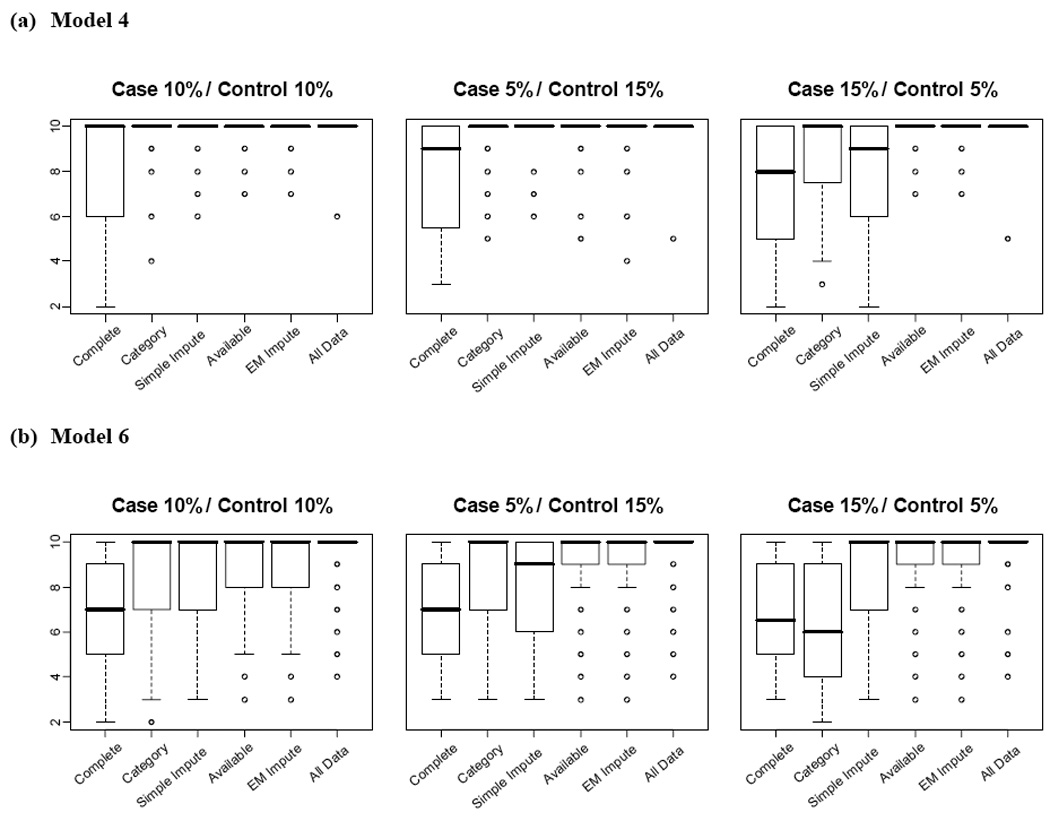
Box plots of cross validation consistency for datasets of (a) Model 4 and (b) Model 6. The boxes represent interquartile ranges. The circles are points beyond 1.5 interquartile ranges from the box.

In order to evaluate how efficiently the ORs were estimated at the last step of MDR, the distributions of log ORs for individual genotype combinations were compared (Figure 4). The true values of the ORs were calculated from the given penetrances and genotype frequencies for each genotype combination of the two causal loci. The distributions of the estimated ORs varied much depending on genotype combination and the approaches used (data not shown). However, the estimates of the ORs from Complete tended to show large variances and Missing Category yielded large biases in some cases. Figure 4 shows box plots of the log ORs for the specific genotype combination having the largest sample frequency. These box plots were derived from the 100 log ORs from the 100 replicate datasets of Models 4 and 6. The horizontal dashed lines represent the true values of the log ORs. The results showed that the variance of log OR using Complete was larger than those using the other approaches. In particular, for both Models 4 and 6, log ORs using Missing Category were highly biased when the missing rates were unbalanced. When the missing rate in controls was higher than that in cases, say (5%, 15%), Missing Category led to ORs with positive biases. When the missing rate in controls was smaller than that in cases, say (15%, 5%), Missing Category led to ORs with negative biases. On the other hand, Available and EM Impute approaches provided unbiased estimates of the ORs in these situations. Simple Impute showed small variances but highly biased estimates for some situations, such as missing rates (15%, 5%) in Model 4.

Fig. 4.

Box plot of log OR estimates for the combination of major homozygote genotypes of the simulated causal loci from (a) Model 4 and (b) Model 6. Horizontal dashed line indicates the true value. Boxes and circles are defined as for Fig. 3.

We also computed the mean squared error (MSE) of the OR estimate, i.e. the sum of the variance and squared bias (data not shown). Complete, Missing Category, and Simple Impute approaches tended to yield highly variable MSEs, depending on the penetrance model of the data and the missing rates. On the other hand, Available and EM Impute gave very similar MSEs to those of AllData and thus consistently yielded small MSEs.

In summary, our simulation study showed that Complete performed worst, losing power severely as the missing rate increased. Missing Category tended to yielded low power when the missing rates were unbalanced. Simple Impute had less power than Available and EM Impute approaches, but the power reduction was milder than that for the Complete or Missing Category approaches. Available and EM Impute approaches performed equally well in all cases. Moreover, they estimated the OR with good precision and accuracy, which improved the classification into high-risk/low-risk groups.

Analysis of Atopic dermatitis data

Data were obtained from the genetic association study of atopic dermatitis that was conducted at the Skin Disease Genomic Research Center of Samsung Medical Center in Korea. Atopic dermatitis is a chronic inflammatory skin disease that leads to significantly deteriorated life quality. An earlier twin study indicated that atopic dermatitis is strongly genetic with an enhanced level of concordance reported in monozygotic relative to dizygotic twins (0.72–0.77 vs. 0.15–0.23) [Schultz Larsen 1993]. The fact that the monozygotic concordance is so much larger than the dizygotic concordance is suggestive of epistatic interactions [Risch 1990]. Our data consisted of 284 atopic dermatitis patients and 188 normal subjects. A total of twenty SNPs were genotyped from three genes: sphingomyelin phosphodiesterase 2 (SMPD2), GATA binding protein 3 (GATA3) and signal transducer and activator of transcription 6 (STAT6). The detailed experimental procedures are described in Kim, et al. [2007]. Information on the SNPs, such as location, minor allele frequency and missing rates in cases and controls is shown in Table 2. The missing rates are 5.6% for cases and 1.8% for controls. The overall average missing rate is 4%.

Table 2.

Information on the SNPs with missing rates in cases and controls.

ID	Position	Function	Alleles	MAF1	HWE2	Missing rate
						Case (n=284)	Control (n=188)
SMPD2_1	−318C>T	Exon1	C/T	0.040	0.850	30% (86)	12% (22)
SMPD2_2	−89G>A	Exon1	G/A	0.368	0.987	4% (12)	1% (2)
SMPD2_3	+8C>T	Exon1	C/T	0.197	0.134	4% (12)	1% (1)
SMPD2_4	+276A>C	Exon2	A/C	0.103	0.989	5% (15)	2% (4)
SMPD2_5	+716G>C	Intron3	G/C	0.170	0.999	6% (18)	1% (2)
SMPD2_6	+1231C>T	Intron5	C/T	0.083	0.794	4% (12)	1% (1)
SMPD2_7	+1898G>A	Exon8	G/A	0.015	0.983	2% (7)	1% (2)
SMPD2_8	+2080C>T	Intron8	C/T	0.043	0.902	4% (11)	0% (0)
GATA3_1	−1420G>A	Promoter	G/A	0.051	0.849	3% (8)	0% (0)
GATA3_2	−251A>G	Promoter	A/G	0.405	0.273	5% (13)	2% (4)
GATA3_3	+8735G>A	Intron3	G/A	0.305	0.721	7% (20)	3% (6)
GATA3_4	+8841T>C	Intron3	T/C	0.344	0.278	5% (14)	2% (3)
GATA3_6	+18461C>T	Exon5	C/T	0.284	0.925	4% (11)	2% (4)
STAT6_1	+2804G>A	Exon8	G/A	0.029	0.509	2% (7)	1% (2)
STAT6_2	+8460C>T	Exon15	C/T	0.004	0.997	5% (14)	1% (1)
STAT6_3	+9066C>T	Intron16	C/T	0.252	0.459	6% (18)	0% (0)
STAT6_4	+9317C>T	Intron17	C/T	0.161	0.753	2% (6)	1% (2)
STAT6_5	+11962A>G	Exon22	A/G	0.427	0.782	4% (11)	2% (3)
STAT6_6	+12353A>G	Exon22	A/G	0.072	0.635	4% (11)	3% (5)
STAT6_7	+12414G>A	Exon22	G/A	0.277	0.348	5% (13)	2% (3)

¹Minor Allele Frequency

²Hardy Weinberg Equilibrium test p-value

For illustrative purposes, we focus only on two-locus models. To identify the second order interactions, we applied the five approaches described in Section 2. Missing Category chose (SMPD2_1, GATA3_2) as the best SNP combination. Simple Impute chose (SMPD2_3, GATA3_4) as the best SNP combination. All other three approaches selected the same two-locus model (SMPD2_3, GATA3_2) as the best SNP combination.

SMPD2_1 had an unusually high missing rate: 30% for cases and 12% for controls, showing large imbalance between the two groups. These missing rates are much larger than those of the other SNPs. Because of its large missing rates, our earlier analysis in Kim, et al. [2007] excluded this SNP. In this analysis, we intentionally included it to evaluate the MDR approaches. When we reanalyzed the data after removing SMPD2_1, the same best model (SMPD2_3, GATA3_2) was also obtained by using Missing Category. This example shows that the conclusion based on Missing Category may be misleading when the missing rates are unbalanced between cases and control groups.

Now, we further focus on results of Available and EM Impute approaches. Note that both approaches were shown to perform better than other approaches in simulation studies. From 10-fold cross validation, Available and EM Impute approaches yielded the same CVC 9/10 and similar testing BAs 55.709 and 54.711, respectively. Table 3 shows the ORs and their 95% CIs for each genotype combination of (SMPD2_3, GATA3_2). Both approaches resulted in similar ORs. When the 95% CI of OR for a given genotype combination does not include the value 1, that combination has a significantly positive or negative effect on the occurrence of disease at the 5% significance level. The confidence intervals of (CC, GG) did not include 1 for both approaches, implying that (CC, GG) has a significantly high risk. Although the effect of the interaction of SMPD2_3 and GATA3_2 on atopic dermatitis needs to be further analyzed to obtain a fuller biological interpretation, this example illustrates the effect of the missing genotypes on the gene-gene interaction analysis using MDR.

Table 3.

Summary of the odds ratios and their 95% confidence intervals for the genotype combinations of the (SMPD2_3, GATA3_2)

(SMPD2_3, GATA3_2)	Risk group	Available		EM Impute
		Case : Control	OR (95%CI)	Case : Control	OR (95%CI)
(CC, AA)	High	57 : 35	1.133 (0.778,1.651)	62.1 : 35.8	1.146 (0.787,1.67)
(CT, AA)	Low	30 : 27	0.773 (0.476,1.255)	32.2 : 28.7	0.743 (0.459,1.201)
(TT, AA)	High	5 : 2	1.74 (0.341,8.869)	5.2 : 2	1.706 (0.33,8.823)
(CC, AG)	Low	75 : 70	0.746 (0.572,0.972)	81.1 : 70.6	0.76 (0.582,0.993)
(CT, AG)	High	42 : 26	1.124 (0.716,1.765)	44.7 : 27.2	1.089 (0.694,1.708)
(TT, AG)	High	4 : 1	2.783 (0.314,24.701)	4.2 : 1	2.75 (0.3,25.214)
(CC, GG)	High*	39 : 9	3.015 (1.498,6.071)	42.8 : 9.1	3.119 (1.542,6.309)
(CT, GG)	Low	8 : 13	0.428 (0.181,1.012)	8.6 : 13.6	0.421 (0.179,0.992)
(TT, GG)	High	3 : 0	∞	3.2 : 0	∞
Total ratio		263 : 183		263 : 183**

^*The 95% CIs do not include the value one for any of the approaches

^**Imputed cell frequencies were scaled to make the total cell frequency equal to the total observed cell frequency

SUMMARY & DISCUSSION

The MDR method has several advantages in the analysis of gene-gene interactions for an association study. For example, it does not require the assumption of the mode of genetic inheritance and can be applied when sample sizes are small [Motsinger and Ritchie 2006]. However, not many studies have been done on MDR analysis with missing observations. In this study, we showed that the commonly used approaches to handle missing values in MDR analysis, such as Complete, Missing Category, and Simple Impute, have low power when the missing rates are large or the missing rates are unbalanced between the case and control groups.

Available and EM Impute approaches account for missing genotypes in the analysis of gene-gene interactions with little loss of information. In particular, EM Impute estimates missing genotype cell frequencies using the EM algorithm. It uses all the available information for a given dataset in the presence of missing values and avoids the sparseness problem as much as possible. In the simulation study, Available and EM Impute approaches showed high empirical power in terms of detecting true causal loci, with high CVCs. Complete performed worse, incurring severe loss of power. The power loss increased as the total missing rate increased. Missing Category, in which missing is treated as an additional genotype category, showed comparable power to Available and EM Impute when the missing rates are balanced between cases and controls. When the missing rates of cases and controls are unbalanced, however, Missing Category tended to choose non-causal models and yielded low power, while EM Impute and Available performed equally well. Although it lost power as missing rates increased, Simple Impute lost less power than did Complete and Missing Category. In practice, Simple Impute is recommended over Complete and Missing Category for the analysis of incomplete data (http://compgen.blogspot.com). Although Simple Impute performed reasonably well for the lower missing rates, it was less powerful than Available and EM Impute. In conclusion, we recommend using EM Impute or Available investigate gene-gene interactions when there are missing data.

In the present study, Available performed almost as powerfully as EM Impute. Further study is desirable to assess which of these two performs better for higher order interaction analysis. In this study, we generated missing values under the assumption that the missing mechanism follows the missing completely at random (MCAR) assumption [Little and Rubin 2002]. In a future study, different missing data mechanisms, such as missing at random (MAR) or not missing at random (NMAR), will be considered. These missing data mechanisms may produce some differences between Available and EM Impute approaches.

The EM algorithm is known to converge well for the exponential family of distributions. This convergence property of the EM algorithm was shown by Dempster et al. [1977] and further addressed by Wu [1983]. Since our approach assumes the multinomial distribution for the observed cell frequencies, the EM algorithm does not suffer from any convergence problem. Further, since we assume a very simple missing data mechanism, it converged with a small number of iterations. Although EM converges relatively fast, the additional computation in EM Impute may impact on the analysis of large scale genotype data. To avoid a computational burden, we considered a one-step EM Impute approach which iterates only one step of the EM algorithm. Its performance was almost as good as the fully iterated EM Impute approach in terms of power (data not shown).

In order to investigate the impact of adding the imputation procedure, we have investigated the computation times using the real data example as well as simulated datasets. We used our software ImputeMDR written in the R language which can be downloaded through CRAN on the R web site (http://www.r-project.org/). We compared the computation times of Missing Category, Available, and EM Impute. First, we analyzed the real data example of atopic dermatitis dataset. The computation time was measured by using a desktop PC with 1.86GHz CPU and 1Gb memory. For second-order interaction, there were no differences in computation times among the three approaches. For third-order interaction, EM Impute took more times than others. However, its computation time was less than one second.

Next, we investigated the computing times for the second-order, third-order, and fourth-order interactions using the simulated datasets. We varied the number of SNPs from 10 to 50, and the missing rate from 1% to 10%. We also varied the total sample size from 200 to 2,000. Figure 5 (a) shows how the computing time changes over the number of SNPs for the case when the sample size is 400 and the missing rate is 5%. In general, as the number of SNPs increases, the computation times of all approaches increase. Figure 5 (b) shows how the computing time changes over the missing rate number of SNPs for the case when the sample size is 400 and the number of SNPs is 30. As the missing rate increases, the computation times of Missing Category and Available do not change much, while the computation time of EM Impute increases linearly. Figure 5 (c) shows how the computing time changes over the sample size for the case when the number of SNPs is 30 and the missing rate is 5%. As the sample size increases, the computation times of all approaches increase. Although EM Impute took much more time for third- and fourth-order interactions, the computation time of EM Impute tend to be stabilized as the sample size increases. The computation time of the one-step EM is much smaller than EM Impute but only slightly longer that of Available. Thus, for the association studies using a large number of SNPs, the one-step EM Impute approach might be a good alternative.

Fig. 5.

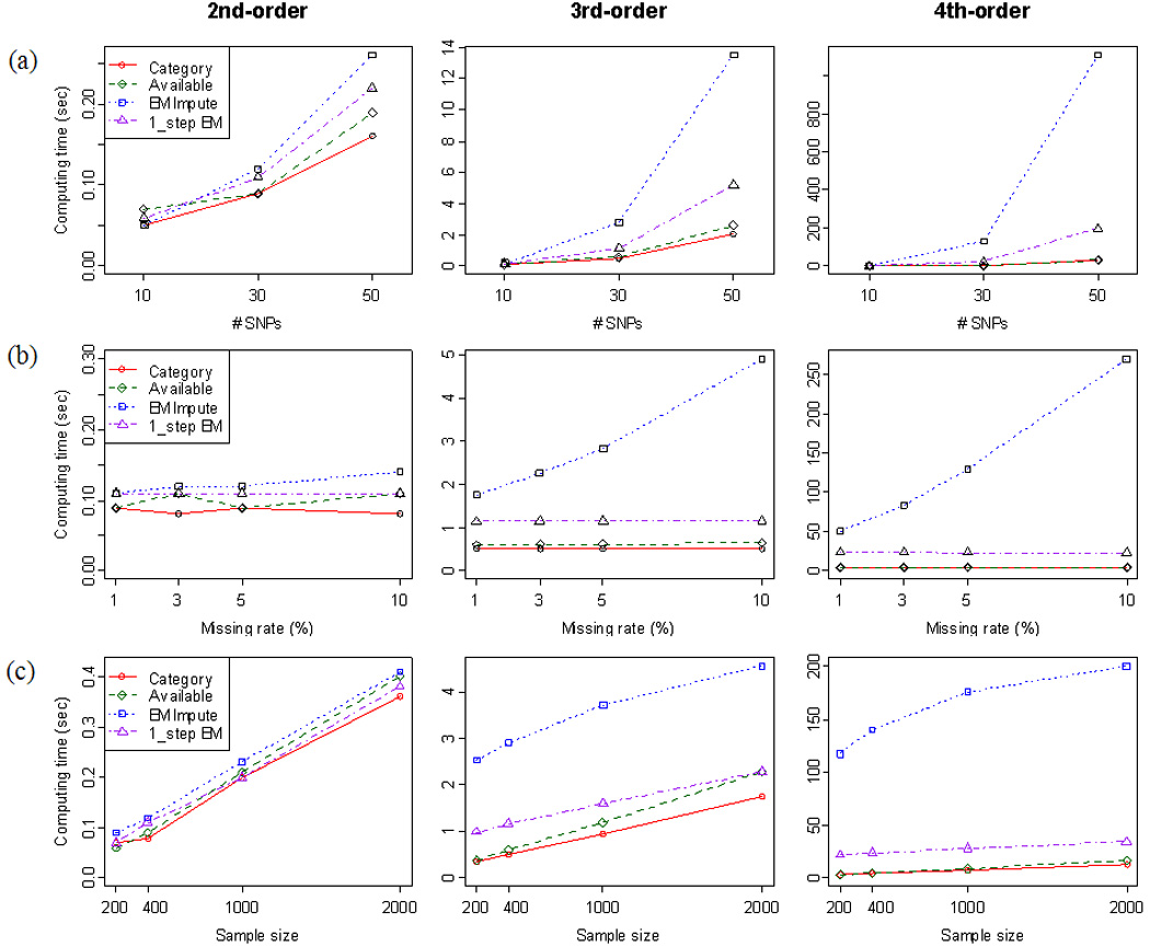
Computation times of the second-order, third-order, and fourth-order interactions using the simulated datasets; (a) the computing times over the number of SNPs for the case when the sample size is 400 and the missing rate is 5%; (b) the computing time over the missing rate number of SNPs for the case when the sample size is 400 and the number of SNPs is 30; 5 (c) the computing time over the sample size for the case when the number of SNPs is 30 and the missing rate is 5%. Experiment is conducted using a PC with Intel 1.86 GHz CPU, 1Gb memory, and Windows XP OS.

In summary, EM Impute tends to have a longer computation time than the other approaches, as the missing rate, the sample size, and the order of interaction increase. However, for the lower order interaction up to the third-order interaction, the computation time of EM Impute is generally very short. Thus, EM Impute can be easily applied to candidate gene analysis without serious computational burden. However, for the association studies using a large number of SNPs such as genome-wide association studies (GWAS), EM Impute might be difficult to apply and Available or one-step EM is recommended.

REFERENCES

- Andrew AS, Nelson HH, Kelsey KT, Moore JH, Meng AC, Casella DP, Tosteson TD, Schned AR, Karagas MR. Concordance of multiple analytical approaches demonstrates a complex relationship between DNA repair gene SNPs, smoking and bladder cancer susceptibility. Carcinogenesis. 2006;27(5):1030–1037. doi: 10.1093/carcin/bgi284. [DOI] [PubMed] [Google Scholar]
- Bush WS, Dudek SM, Ritchie MD. Parallel multifactor dimensionality reduction: a tool for the large-scale analysis of gene-gene interactions. Bioinformatics. 2006;22(17):2173–2174. doi: 10.1093/bioinformatics/btl347. [DOI] [PMC free article] [PubMed] [Google Scholar]
- Chung Y, Lee SY, Elston RC, Park T. Odds ratio based multifactor-dimensionality reduction method for detecting gene-gene interactions. Bioinformatics. 2007;23(1):71–76. doi: 10.1093/bioinformatics/btl557. [DOI] [PubMed] [Google Scholar]
- Dempster AP, Laird NM, Rubin DB. Maximum Likelihood from Incomplete Data via the EM Algorithm. Journal of the Royal Statistical Society. Series B. 1977;39(1):1–38. [Google Scholar]
- Hahn LW, Ritchie MD, Moore JH. Multifactor dimensionality reduction software for detecting gene-gene and gene-environment interactions. Bioinformatics. 2003;19(3):376–382. doi: 10.1093/bioinformatics/btf869. [DOI] [PubMed] [Google Scholar]
- Kim HT, Lee JY, Han BG, Kimm K, Oh B, Shin HD, Namkung JH, Kim E, Park T, Yang JM. Association analysis of sphingomyelinase 2 polymorphisms for the extrinsic type of atopic dermatitis in Koreans. J Dermatol Sci. 2007;46(2):143–146. doi: 10.1016/j.jdermsci.2006.12.001. [DOI] [PubMed] [Google Scholar]
- Little RJA, Rubin DB. Statistical Analysis with Missing Data. Second Edtion. Wiley-Interscience; 2002. [Google Scholar]
- Moore JH. The ubiquitous nature of epistasis in determining susceptibility to common human diseases. Hum Hered. 2003;56(1–3):73–82. doi: 10.1159/000073735. [DOI] [PubMed] [Google Scholar]
- Moore JH, Gilbert JC, Tsai CT, Chiang FT, Holden T, Barney N, White BC. A flexible computational framework for detecting, characterizing, and interpreting statistical patterns of epistasis in genetic studies of human disease susceptibility. J Theor Biol. 2006;241(2):252–261. doi: 10.1016/j.jtbi.2005.11.036. [DOI] [PubMed] [Google Scholar]
- Moore JH, Williams SM. New strategies for identifying gene-gene interactions in hypertension. Ann Med. 2002;34(2):88–95. doi: 10.1080/07853890252953473. [DOI] [PubMed] [Google Scholar]
- Motsinger AA, Ritchie MD. Multifactor dimensionality reduction: an analysis strategy for modelling and detecting gene-gene interactions in human genetics and pharmacogenomics studies. Hum Genomics. 2006;2(5):318–328. doi: 10.1186/1479-7364-2-5-318. [DOI] [PMC free article] [PubMed] [Google Scholar]
- Qin ZS, Niu T, Liu JS. Partition-ligation-expectationmaximization algorithm for haplotype inference with singlenucleotide polymorphisms. Am J Hum Genet. 2002;71:1242–1247. doi: 10.1086/344207. [DOI] [PMC free article] [PubMed] [Google Scholar]
- Risch N. Linkage strategies for genetically complex traits. I. Multilocus models. Am J Hum Genet. 1990;46(2):222–228. [PMC free article] [PubMed] [Google Scholar]
- Ritchie MD, Hahn LW, Moore JH. Power of multifactor dimensionality reduction for detecting gene-gene interactions in the presence of genotyping error, missing data, phenocopy, and genetic heterogeneity. Genet Epidemiol. 2003;24(2):150–157. doi: 10.1002/gepi.10218. [DOI] [PubMed] [Google Scholar]
- Ritchie MD, Hahn LW, Roodi N, Bailey LR, Dupont WD, Parl FF, Moore JH. Multifactor-dimensionality reduction reveals high-order interactions among estrogen-metabolism genes in sporadic breast cancer. Am J Hum Genet. 2001;69(1):138–147. doi: 10.1086/321276. [DOI] [PMC free article] [PubMed] [Google Scholar]
- Scheet P, Stephens M. A fast and flexible statistical model for large-scale population genotype data: applications to inferring missing genotypes and haplotypic phase. Am J Hum Genet. 2006;78(4):629–644. doi: 10.1086/502802. [DOI] [PMC free article] [PubMed] [Google Scholar]
- Schultz Larsen F. Atopic dermatitis: a genetic-epidemiologic study in a population-based twin sample. J Am Acad Dermatol. 1993;28(5 Pt 1):719–723. doi: 10.1016/0190-9622(93)70099-f. [DOI] [PubMed] [Google Scholar]
- Sherriff A, Ott J. Applications of neural networks for gene finding. Adv Genet. 2001;42:287–297. doi: 10.1016/s0065-2660(01)42029-3. [DOI] [PubMed] [Google Scholar]
- Tahri-Daizadeh N, Tregouet DA, Nicaud V, Manuel N, Cambien F, Tiret L. Automated detection of informative combined effects in genetic association studies of complex traits. Genome Res. 2003;13(8):1952–1960. doi: 10.1101/gr.1254203. [DOI] [PMC free article] [PubMed] [Google Scholar]
- Velez DR, White BC, Motsinger AA, Bush WS, Ritchie MD, Williams SM, Moore JH. A balanced accuracy function for epistasis modeling in imbalanced datasets using multifactor dimensionality reduction. Genet Epidemiol. 2007;31(4):306–315. doi: 10.1002/gepi.20211. [DOI] [PubMed] [Google Scholar]
- Wolf JB, Brodie ED, Wade MJ. Epistatsis and the Evolutionary Process. Oxford University Press; 2000. [Google Scholar]
- Zhang H, Bonney G. Use of classification trees for association studies. Genet Epidemiol. 2000;19(4):323–332. doi: 10.1002/1098-2272(200012)19:4<323::AID-GEPI4>3.0.CO;2-5. [DOI] [PubMed] [Google Scholar]