New methods in Diffusion Weighted and Diffusion Tensor Imaging

Synopsis

Considerable strides have been made by countless individual researchers in diffusion-weighted imaging (DWI) to push DWI from an experimental tool – limited to a few institutions with specialized instrumentation – to a powerful tool used routinely for diagnostic imaging. Despite its current success, the field of DWI constantly evolves and progress has been made on several fronts, awaiting adoption by vendors and clinical users to bring in the next generation of DWI. These developments are primarily comprised of improved robustness against patient and physiologic motion, increased spatial resolution, new biophysical and tissue models, and new clinical applications for DWI. This article aims to provide a succinct overview of some of these new developments and a description of some of the major challenges associated with DWI. Trying to understand some of these challenges is helpful not only to the technically savvy MRI user, but also to radiologists who are interested in the potential strengths and weaknesses of these techniques, what is in the “diffusion pipeline”, and in how to interpret artifacts on DWI scans.

1. Introduction

During the past decade, diffusion-weighted MRI (DWI) has matured into a powerful and extensively-used diagnostic tool, and has entered the diagnostic arena mostly due to its superb sensitivity to ischemic stroke¹ during the early time window where other MR methods and CT are still negative². DWI relies on using the biophysical property of proton (self-)diffusion as contrast-determining parameter in an MRI experiment. Due to the presence of restricting cellular structures, diffusion in biological tissue is often anisotropic. That is, the diffusion coefficient is different when measured along different directions; for example, in white matter diffusion is higher along fibers and lower perpendicular to fibers. Thus, anisotropic diffusion can be used as a sensitive proxy measure for structural integrity of the underlying neural tissue and for non-invasive neuronal tract tracing. In muscle fibers, for example, diffusion anisotropy can be used to determine the pennation angle of muscle fibers (that is, s the angle formed by the individual muscle fibers with the line of action of the muscle) allowing one to investigate biomechanical properties of muscles.

Advancements in DWI, such as q-space imaging³ but most importantly diffusion tensor imaging (DTI)⁴, have demonstrated great utility in furthering the diagnostic potential of MRI to reveal tissue features otherwise occult to conventional MRI; even simple variants to DWI, such DWIBS⁵, have opened new perspectives on how DWI can be utilized beyond stroke work-up.

However, DWI and its variants are still poised with major challenges when it comes to resolution, distortion, and at higher magnetic field strengths. The problems arise from the continued dependence on rapid single-shot echo-planar imaging (ssEPI) and DWI's motion sensitivity. In this article, we will attempt to provide a brief overview of these challenges and some new concepts that have been developed to address these problems.

2. Basic Principles

Diffusion is generally a 3D phenomenon and can vary in magnitude depending on the direction along which it is measured. The effect of molecular diffusion in an MR experiment was first described by Torrey⁶, who noted that, in the presence of a diffusive spin movement in a strong magnetic gradient field, the signal becomes attenuated. In DWI a spin-echo sequence is usually used with a pair of strong diffusion-weighting gradients straddling the 180° refocusing pulse (Fig. 1). This sequence is known as Stejskal-Tanner pulse sequence⁷. The degree of attenuation depends on the strength (G_Diff) and duration (δ) of the diffusion-encoding gradients, the spacing between these gradients (Δ), the apparent diffusion coefficient (ADC), and the gyromagnetic ratio (γ) (implying that, for example, hyperpolarized Xe-gas will experience less attenuation from diffusion than protons due to its lower γ value). Increases in any of those parameters will lead to a reduction in the MR signal intensity. The diffusion-weighting applied is represented by the diffusion attenuation factor or simply the “b”-value:

Figure 1.

Spin-echo sequence with diffusion-weighted gradients (GDiff) - also known as a Stejskal-Tanner sequence.

$$b={\gamma }^2{\text{G}}_{{\text{Diff}}^2}{\delta }^2(\Delta -\delta /3),$$ [1]

so that the signal equation of a diffusion-weighted sequence becomes

$$M(b)=M_0·\text{exp}(-b·\text{ADC}),$$ [2]

where M₀ is the spin-echo signal (including proton density and/or any T1/T2 relaxation) in the absence of any diffusion-weighting. From phase-contrast MRI many of the readers are probably familiar with the phase accrual that occurs when spins are moving along a magnetic field gradient and might therefore wonder why there is no net phase accrual associated with the diffusion process. Such phase does accumulate in spin ensembles with bulk motion, but diffusion is a random process without any coherent motion, so the phase accrual takes place on a per-spin basis. In other words, each diffusing spin follows its own random pathway and will accrue its own phase. For an ensemble of spins the displacement probability function (PDF) has a Gaussian dsitribution and so is the PDF for the phase. Thus, when summed over all spins within a voxel, all these individual phases will integrate to a net attenuation of the signal without a net phase accrual measurable to the outside world. However, in vivo exams are frequently corrupted with bulk motion, which – unlike diffusion – is coherent and leads to unpredictable phase terms that have challenged investigators for a long time.

Within pure water or CSF, diffusion is unrestricted and the measured diffusion constant is independent of the direction along which the ADC was measured. If diffusion is isotropic, there is no preferred direction of water motion for these tissues. However, as mentioned above diffusion can be directionally dependent in biological tissues. The directionality of diffusion is introduced because water movement in and around cellular structures is not “free” as it is in a bulk fluid; it is restricted as it comes into contact with cell membranes and other large structures. This directional dependence, i.e. diffusion anisotropy, is the hallmark of another underlying diagnostic feature of DWI. It was Basser^{4, 8} who recognized that the anisotropy of measured diffusivity in tissue at each point in space (r=[x y z]^T) should be modeled as a second order tensor,

$$\begin{array}{cccc}& D{(\text{r})}_{xx}& D{(\text{r})}_{xy}& D{(\text{r})}_{xz}\\ \underset{\_}{\underset{\_}{\text{D}}}(\text{r})=& D{(\text{r})}_{yx}& D{(\text{r})}_{yy}& D{(\text{r})}_{yz}\\ & D{(\text{r})}_{zx}& D{(\text{r})}_{zy}& D{(\text{r})}_{zz},\end{array}$$ [3]

and devised a data acquisition scheme that goes along with it. Since the diffusion tensor is symmetric (i.e. D_ij = D_ji), only six unknown elements need to be determined in each voxel. Specifically, a diffusion tensor MRI (DTI) experiment in which these elements are determined on a per pixel basis consists of acquiring a series of DWI scans, each with gradients applied along a different direction. Specifically, to estimate the tensor requires the acquisition of at least six DWI scans together with a non-diffusion-weighted image for reference. In practice, in order to improve to estimation of the diffusion tensor, many more than six directions are often acquired with the diffusion directions spread isotropically over a sphere (Fig. 2). Although this process appears intuitively trvial, this so-called “tessellation” process is mathematically challenging^{9, 10}. Since any extra encoding direction adds extra time, a tradeoff is often sought between the optimum number of directions and acceptable scan time. A few tens of directions will already improve the image quality of the tensor estimations and to avoid orientational bias¹¹. If one elects to choose just the minimum 6 directions, care must be taken that these directions are noncollinear.

Figure 2.

Isotropic distribution of 256 diffusion-encoding directions over a sphere. Each bump on the sphere represents the point where the diffusion-encoding vector (starting at the origin) penetrates the isosphere.

The directionality of diffusion is performed by combining the x, y, and z magnetic field gradients such that the superposition of these individual gradients will lead to a net field gradient along the direction vector defined by g_Diff=[G_Diff,x G_Diff,y G_Diff,z]^T, where G_Diff, i (i=x,y,z) is the gradient strength applied along the principal direction. Assuming the aforementioned diffusion tensor model, for a particular diffusion-encoding direction, g_Diff, Eq 2 can be modified accordingly:

$$M(\underset{\_}{\underset{\_}{\text{b}}})=M_0\text{exp}{-}_0^{TE}\left({\text{k}}^T(t)\cdot \underset{\_}{\underset{\_}{\text{D}}}\cdot \text{k}\left(t\right)\right)dt=M_0\text{exp}(\underset{\_}{\underset{\_}{\text{b}}}\cdot \underset{\_}{\underset{\_}{\text{D}}}),$$ [4]

with

$$\text{k}\left(t\right)={\gamma }_0^t{\text{g}}_{\text{Diff}}(\tau )d\tau .$$ [5]

From the six or more DW images acquired with the diffusion-encoding along different gradient directions, the elements of D͇(r) can be calculated by simple regression analysis⁴. Since it is normally sufficient to use a single directional DWI measurement (or at most 3 measurements along orthogonal directions to avoid confounding signal nonuniformities from anisotropic stuctures) to identify regions of reduced ADC in acute stroke patients, one might wonder about the utility of measuring the entire tensor. By making an extra effort to measure all elements of the tensor, one can derive certain properties in each voxel, such as the extent of diffusion anisotropy or the direction in which the diffusion is highest.

To be able to interpret the tensor information, it is necessary to break down this information into single-valued measures that can be viewed as gray scale maps readable to the radiologist. In order to calculate these measures, the diffusion tensor D͇ is first diagonalized, which is a standard mathematical matrix operation that rotates the coordinate frame of reference independently - pixel-by-pixel - into the principal axes of the tensor. By doing so, the so-called eigenvalues λ₁, λ₂, and λ₃ as well as the orientation of the diffusion tensor are explicitly obtained by the so-called eigenvectors e₁, e₂, and e₃. The mean diffusivity is then calculated by

$$\langle D\rangle =\left({\lambda }_1+{\lambda }_2+{\lambda }_2\right)/3,$$ [6]

where the numerator of Eq 6 is the “trace” of the matrix D͇, and the relative diffusion anisotropy, RA, as

$$\text{RA}=\frac{\sigma ({\lambda }_1,{\lambda }_2,{\lambda }_3)}{\langle D\rangle },$$ [7]

which is the standard deviation of the eigenvalues divided by their mean. Alternatively, RA can be seen as relating the magnitude of the anisotropic portion of the tensor to the magnitude of the isotropic portion of D͇. Note that the eigenvectors provide information about direction of the maximum diffusion within a voxel on which fiber tracking^{12, 13} will build upon. There are other rotationally-invariant scalar metrics that describe the diffusion anisotropy, most of which have different sensitivity to different ranges of diffusion anisotropy. Here, rotationally-invariant refers to the property that such measures are independent of the orientation of the diffusion tensor. The most commonly used measure for diffusion anisotropy is fractional anisotropy (FA):

$$FA=\sqrt{\frac{\text{1}}{2}}\frac{\sqrt{{({\lambda }_1-{\lambda }_2)}^2+{({\lambda }_2-{\lambda }_3)}^2+{({\lambda }_3-{\lambda }_1)}^2}}{\sqrt{{\lambda }_1^2+{\lambda }_2^2+{\lambda }_3^2}},$$ [8]

where FA measures the fraction of the magnitude of D͇ that is anisotropic by looking at the ratio between the magnitude of the deviatoric tensor, D͇=D͇-<D>, and the full tensor.

While the second-order diffusion tensor model served us well for almost ten years, alternative models have become increasingly popular. Most of them address the fact that in biological tissue a complex interplay between different compartments and structures inside a voxel pose different amounts of hindrance to the diffusing spins. While the second order tensor is often illustrated as an ellipsoid (n.b. the surface of the ellipsoid depicts the displacement front of protons), the true representation for a high-angular diffusion experiment, where diffusion is measured along many directions in space, rather resembles a more wrinkled structure.

High-angular resolution DWI (HARDI) ^{14, 15} was one of the first attempts to tackle the problem of the more complex diffusive spin displacement. Here, the 3D structure spanned by the ADC measurements was decomposed along different directions into three-dimensional basis functions (so-called spherical harmonics). By applying directional ADC measurements, however, an underlying Gaussian spin-displacement PDF was inherently assumed.

In fact, the complex interplay of countless structures within in a voxel renders the true spin displacement PDF to be a non-Gaussian distribution and may not even be symmetric. To measure the PDF or a ‘diffraction pattern’, Callaghan introduced the concept of q-space imaging^{3, 16}. This required extremely short and strong gradients only available on small-bore experimental systems. Nevertheless, Callaghan's method was adapted for the use in neuronal tissue¹⁷ and in-vivo¹⁸. Realizing that the spin displacement PDF in-vivo requires measurements along many directions and at many different b-values, Wedeen et al.^{19, 20} proposed a scheme to obtain an approximate measurement of the 3D displacement PDF in each voxel, known as diffusion spectrum imaging (DSI), which was then further approximated and compacted by Tuch with the introduction of Q-ball imaging²¹.

Following our initial discussion about how a Gaussian spin displacement PDF will lead to an attenuation of the signal (and a second-order tensor) when averaged over the entire spin ensemble, the “DWI-connoisseur” will realize that for non-Gaussian PDFs the ensemble average will lead to signal contributions that can be expressed by higher order tensors²² (Fig. 3). In fact, if the spin displacement PDF is asymmetric, additional phase terms exist²².

Figure 3.

Zoomed glyph visualization of spin displacement isospheres (minus isotropic component) derived from higher order diffusion tensors from a human volunteer brain (see insert box). For better contrast, an FA map is plotted underneath. Clearly, the isospheres deviate from the typically seen diffusion ellipsoids, which is most prominent in regions of merging or crossing fiber tracts.

3. Problems with Motion-Induced Phase Errors

One of the greatest technical challenges for diffusion-weighted imaging (DWI) is overcoming the phase effects originating from coherent macroscopic or bulk motion, while retaining its sensitivity to microscopic motion. To create diffusion-dependent contrast, DWI pulse sequences must be sensitive to incoherent molecular motion on the order of a few microns. The price for the sensitivity to motion on this microscopic scale is that even very small (submillimeter) displacements of tissue during the diffusion-encoding period will cause signal loss and large phase changes in the resulting echo signal. The two major sources of bulk motion are i) periodic tissue motion caused by cardiac pulsatility and ii) patient movement. Because coherent motion on this level is likely to be different during each echo acquisition, the phase of the echo in a standard spin-warp acquisition will be perturbed differently and in an unpredictable fashion - ultimately leading to devastating ghosting artifacts in the final images. The additional phase impressed on the spins will also challenge the phase requirements between transverse magnetization and radio-frequency (RF) pulses for FSE. For this reason, single shot methods such as echo planar imaging (EPI) must be used to avoid the phase variation from shot to shot that can cause ghost artifacts.

3.1. Influence of Phase Errors on Spatial Encoding

As mentioned above, coherent motion in the tissue sample during the diffusion preparation time will lead to through-plane signal dephasing and leave localized phase on the object being imaged prior to the image readout module. Even in cooperative patients, peristalsis, respiratory motion, and pulsatile flow^{23, 24} will confound diffusion imaging and most likely corrupt image quality. To address this issue, the diffusion-weighted images are often acquired with cardiac triggering, i.e. synchronized with the heart rate measured either with ECG or simply by a plethysmograph on a finger. In this way, imaging can be synchronized with the cardiac cycle, and imaging during systole (during which motion is usually highest) can be avoided. However, this prospective triggering approach considerably cuts down the scan efficiency especially when the heart rate goes up, because the quiescent time available for scanning decreases. Respiratory motion during DWI can be even more problematic, especially for body applications. In our practice, breath-hold studies have proven reliable for most DWI studies outside the CNS²⁵. In kidney studies, where a large cranio-caudal movement of the kidneys over the respiration period can be observed, breath-hold experiments are extremely useful. Figure 4 shows an example of such a study in a patient with obstructive kidney disease. The tumor mass led to critically low blood flow to the kidney as indicated by the corresponding MRA. The ADC reduction in the ischemic kidney was dramatic and - to the authors' knowledge - rather uncommon for tissue outside the CNS. However, this case suggests that DWI and ADC measurements might become useful in obstructive kidney disease to differentiate between benign renal oligemia and renal ischemia. In this context, we found also that ADC values correlate well with the creatinine level²⁶ (Fig. 5).

Figure 4.

Patient suffering from a renal cell carcinoma in the right kidney. (A) This lesion causes a significant mass effect on the adjacent renal pelvis with resultant right-sided hydronephrosis on HASTE scans (open arrow). (B) The CE-MRA(MIP) shows that the right kidney is heavily hypoperfused. The mass (asterisk) displaces and compresses the right renal pelvis. (C) The right kidney appears extremely hyperintense on the high-b DWI scan. The corresponding ADC values were significantly depleted (∼30-50% compared to normal tissue) which is indicative for ischemic tissue. Conversely, the hydronephrosis in this patient is characterized by an elevated ADC. The renal cell carcinoma appeared very heterogeneous on ADC maps. (D) The kidney was surgically removed immediately after the MRI. The specimen was cut apart in the mid-sagittal plane of the kidney (dash-dotted line). The dashed line shows the contour of the kidney. The dotted line outlines the tumor.

Figure 5.

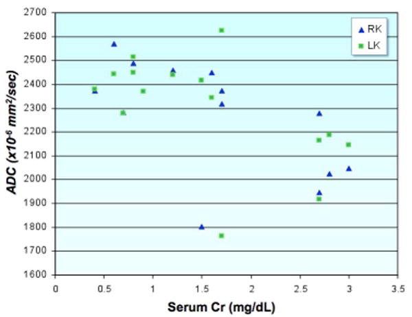
Scatter-plot demonstrating the relationship between serum creatinine levels and renal ADC. Patients with elevated serum creatinine have statistically significant lower renal ADCs. Two patients had unilateral renal disease, which was reflected as markedly decreased ADCs on the affected side - despite only borderline elevation of Cr and normal contralateral renal ADCs. Overall, there was a striking difference in ADCs between normal and compromised kidneys in patients with unilateral renal disease. This technique has great potential for the evaluation of patients with renal disease, particularly those with unilateral disease such as renal artery stenosis and congenital hydronephrosis which may not be reflected in cruder measures of renal function such as serum creatinine.

While the through-plane dephasing results in an overall loss of signal and thus to abnormally high ADC values, the additional spatially non-linear phase imparted by motion conflicts with the phase terms impressed on the transverse magnetization from regular image encoding and leads to considerable ghosting artifacts if not corrected.

Before we continue discussing the phase error problem for image encoding it is important to mention two other issues that need to be considered when applying DWI outside the CNS. These challenges include the presence of lipids within the tissue (e.g. liver, vertebral bodies, or breast) and blood flow: (i) While lipids are normally suppressed to avoid large chemical shift artifacts, the presence of lipids change with age (e.g. breast, vertebral bodies) and disease (e.g. metastatic infiltration, steatosis). Although lipid suppression or water-only excitation suppresses the signal of lipids, the presence of the rather rigid lipid molecules presents more or less hindrance to the diffusing water protons and thus indirectly confounds ADC measurements; (ii) Although intravoxel incoherent motion (IVIM) was initially used for blood flow measurements, the blood volume in brain tissue is only 2-4% and thus the contamination from flow on the diffusion attenuation curve (that is, MR signal over b-value) is rather small. However, the blood volume in other organs, such as the kidneys, can be much higher. Instead of using a b=0 sec/mm² scan as reference, it is often advisable to use a small b-value (e.g. ∼50 sec/mm²) as reference point to avoid overestimating the ADC or make ADC measurements confounded by blood flow. Now let us return to the phase problems.

In DWI, unless single-shot methods are used, k-space data are normally acquired line-byline, or by a subset of lines following a Stejskal-Tanner diffusion-preparation period. Several acquisitions (“multi-shot”) are therefore required to form a fully encoded image. As patient physiologic and bulk motion changes from one preparation period to the next in an unpredictable fashion, so do the additional phase terms imparted on spins^{27, 28}. As a first order approximation we can assume the phase errors are constant and are linear in the image domain. This will shift the desired k-space trajectory by δk_x and δk_y, and add a constant phase δφ; each of which differs from shot to shot (Fig. 6). Unaware of these additional changes to the k-space trajectory, the MR scanner incorrectly stores the acquired MR data in an equidistant data matrix for final image reconstruction and therefore strong ghosting artifacts will appear, which often render the resulting image nondiagnostic.

Figure 6.

(left) desired trajectory of an interleaved (4 interleaves) EPI trajectory. The random phase errors from motion during diffusion-encoding produces – amongst others – linear phase error terms in the image domain. These can be measured with navigator methods. In the k-space domain these linear phase errors are represented as additional shifts of the desired interleaves along k_x and k_y. Thus, the true interleaves are no longer situated on an equidistant grid (center). They are located at arbitrary positions requiring a regridding procedure onto a Cartesian grid or a DFT-based reconstruction. (right) Single-shot also EPI experiences shifts (δk_x, δk_y), but these are the same for each line in k-space. Therefore, they do not cause ghosting artifacts.

For single-shot exams these k-space shifts exist as well, but the entire trajectory itself is shifted and the k-space sampling remains consistent (that is, the originally prescribed sampling density remains) (Fig. 6c). The only thing that needs to be remembered is that for signal averaging or for averaging over diffusion directions, magnitude images must be used (that is, the image phase needs to be cleared) unless one performs phase correction. This is because each single-shot image has its own unique phase impressed and therefore complex averaging, normally used in MR, would lead to destructive interferences in the averaged image (Fig. 7). While a constant and linear phase error model can be used as a relatively good approximation for the phase error problem in DWI, we will see later in this article that a non-linear spatial phase error model characterizes best the real situation.

Figure 7.

(A) Conventional complex signal averaging performed in k-space using single-shot EPI data with diffusion-weighting applied in 4 different diffusion-encoding directions (from left to right). The phase error for each shot leads to destructive interferences in the averaged images. (B) Averaging of the magnitude images removes the destructive interferences.

3.2. Problems with Violating the Meiboom-Gill Condition in FSE

The extra phase impressed on the spins has also considerable implications on how RF pulses can be used following diffusion-contrast preparation. In particular, we are concerned about the spin phase relative to the RF phase of fast spin-echo (FSE) refocusing pulses. FSE has become the workhorse for routine clinical MRI because of its speed, high SNR, and reliability. FSE is robust, and artifacts are uncommon with this sequence. FSE often works well when many other sequences fail. However, for RF pulses in the FSE train that deviate from 180° due to a poor slice profile (these pulses produce flip angles between 0° and the nominal flip angle in the slopes of the slice profile), or when the flip angle is intentionally lowered in an effort to minimize the power deposition in the subject, image artifacts can arise in cases when the transverse magnetization is not aligned with the RF axis of the FSE readout pulses.

These artifacts arise because FSE relies on the amplitude stability of the Carr Purcell Meiboom Gill (CPMG) sequence, which depends on the Meiboom Gill (MG) phase condition²⁹. That is, for an FSE experiment with an interecho time D the MG condition requires the transverse magnetization at a time D\2 prior to the first refocusing pulse to be parallel or antiparallel to the orientation of the subsequent refocusing pulses. If – at D\2 prior to the FSE readout — the magnetization is 90° from the MG phase (non-MG), the emanating signal will decay in amplitude and oscillate over the echo train. Thus, motion in combination with diffusion encoding might produce any phase at point D\2 with unknown amounts of the MG and the non-MG component (Fig. 8). The superposition of both components will lead to unwanted fluctuation in the magnitude of the echoes within the FSE train. Each echo will also incur an additional phase term that is determined by the MG and non-MG component that competes with the desired phase encoding. As a result, diffusion preparation and fast spin-echo readouts have sometimes been deemed incompatible. However, early on, the use of extra crusher gradients has been proposed with the intention to eliminate all but the primary refocused echo component^{30, 31}, since the challenges with the non-MG component arise from higher order echoes and stimulated echoes. Unfortunately, these schemes require large crusher amplitudes that increase linearly with echo number. The added time required to apply the crusher gradients generally becomes prohibitively long after only a handful of echoes. Moreover, spoiling of the CPMG sequence in this way will also cause the echo amplitudes to decrease rapidly with echo number, which increases image blurring (note that much of the signal in FSE is actually from higher order echoes and stimulated echoes). In one of the following sections of this article, two avenues will be discussed that allows DWI to be combined with FSE readouts.

Figure 8.

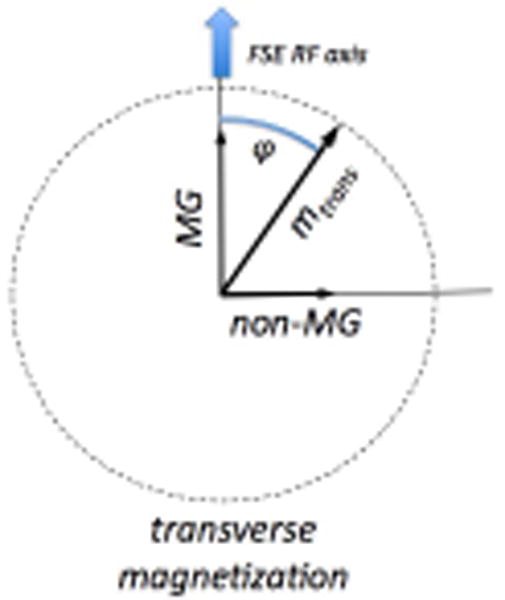
The transverse magnetization following diffusion-preparation will demonstrate an unpredictable phase φ relative to the phase of the subsequent FSE refocusing pulses. The component of the transverse magnetization that is normal to the RF phase of the FSE pulses is called the non-MG component and causes artifacts, whilst the component parallel or anti-parallel to the FSE pulse is the “good” component or MG component.

4. Problems with Echo Planar Imaging

In the previous section it was mentioned that single-shot trajectories are relatively immune against the aforementioned phase errors and therefore minimize or even entirely avoid “ghosting artifacts”. For that reason they have been established as the backbone sequences for DWI. In particular, single-shot echo-planar imaging (EPI)³² and spiral imaging^33-36 (Fig. 9) have been used quite extensively. Until recently, single-shot imaging techniques (especially EPI) were almost exclusively used in the clinical routine. Of particular relevance here is not only single-shot EPI's robustness against phase perturbations but also its extremely fast (for MR standards) image formation capability. For example, using single-shot EPI, each image is acquired within the time frame of 0.1 seconds. This is especially advantageous when thousands of images need to be acquired for DTI or for even more complex acquisition schemes (e.g. GDTI^{37, 38}, HARDI^{14, 15, 39} or q-space^{3, 17, 21, 40}); or for data acquisitions requiring completion within less than 20-25sec (such as in breath-hold exams).

Figure 9.

(A) Diffusion-weighted spin-echo sequence with an EPI readout. Note that the EPI readout shown here is simplified. Typically, many more echoes are acquired for a single-shot EPI scan. (B) Diffusion-weighted spiral sequence.

However, EPI suffers from its own challenges: EPI is limited to low spatial resolution (∼128×128), as well as effects such as image blurring, localized signal loss, and image distortions⁴¹. Image blurring occurs due to the T₂*-based weighting of k-space data around the spin-echo and becomes increasingly pronounced for short T₂* tissues or in poorly shimmed regions. Geometric distortions and signal loss occur predominately at boundaries between tissue and air, due to the local susceptibility differences that lead to an inhomogeneous magnetic field. Over small regions these field changes act as local gradients that compete with the relatively weak spatial encoding gradients along the phase encode dimension (Fig. 10). The extent of these distortions is very dependent on both hardware and how quickly k-space is traversed along the phase encode dimension, as distortions and blurring are proportional to the k-space velocity, vky=dk_y/dt. With increasing field strength these artifacts become more pronounced (Fig. 11). Two single-shot EPI acquisitions can be used, with one acquisition traversing k-space in the opposite direction along the phase encode direction. This enables one to process a distortion field and compute a less distorted image^{42, 43}.

Figure 10.

With EPI the relatively weak net gradients applied along the phase encode direction are offset by local field changes due to susceptibility gradients of comparable magnitude. Thus the effective field deviates from the desired linear change put on by the gradient. Local gradients are stronger (df₁/dr₁) or weaker (df₂/dr₂) than the desired gradient leading to stretched and compressed mapping of voxels, respectively.

Figure 11.

Example for characteristic distortions (arrow) seen with single-shot EPI in adult volunteers at 3T (left) and at 7T (right).

Another effect that impairs image quality in DWI acquired using EPI is the distortions caused by eddy-currents. Eddy currents are unwanted currents in conducting elements of the MR machine counter-acting the rapid switching of the strong and lengthy diffusion-encoding gradients. Depending on the direction along which the diffusion-encoding gradient was applied, the local field changes induced by these eddy currents will cause the images to be hampered by shearing, scaling, translation, or a combination thereof. The net consequence is that individually diffusion-weighted images are misregistered with each other. This is particularly challenging when diffusion tensor information must be processed on a per pixel basis. It often causes scalar maps, such as the diffusion anisotropy, to have erroneous errors (Fig. 12).

Figure 12.

(A-D) images before eddy current distortion correction and (E-H) images after correction. (A, E) reference image: average over all diffusion-weighted images; (B) distorted diffusion-weighted image before correction and (F) afterwards; (C): difference between images A and B: the spatial distortion is seen best around the frontal and posterior cortex (arrows). This is also seen in a map of pixel standard deviation over all diffusion-weighted images (D) as a surrogate measure for diffusion anisotropy. Following distortion correction the difference image between image E and F (G) and the standard deviation map (H) demonstrate that the distortions from eddy currents can be removed.

Since b increases quadratically with the gradient strength, often more than one gradient axis is applied simultaneously to boost the net diffusion-encoding gradient for a given echo time. A very effective encoding scheme is tetrahedral encoding which uses four encoding directions (g₁=[G_x G_y G_z]^T; g₂=[-G_x G_y G_z]^T; g₃=[G_x -G_y G_z]^T; and g₄=[G_x G_y -G_z]^T). Here, all three gradient axes are turned on simultaneously leading to an effective gradient that is $\sqrt{3}{G}_i(i=x,y,z)$. This scheme has proven useful to compute isotropically diffusion-weighted images with little extra time but much improved SNR compared to scans with encoding applied just along the principal gradient direction, i.e. along x, y, and z. However, because more effective gradients are involved, tetrahedral encoding usually demonstrates more eddy current effects than unidirectional encoding. Thus, when DWI scans with diffusion encoding along different directions are combined to compute an isotropically diffusion-weighted image, the resultant image will be blurred if the eddy current-induced distortions are not compensated. Thus, an anatomically consistent DTI data set and derivations thereof (<D>, RA etc.) and a sharp isotropically diffusion-weighted image requires exams where the effects from eddy currents are minimized. This can be achieved either by specific modifications to the standard DWI pulse sequence (e.g. by means of a dual-spin-echo preparation⁴⁴ (Fig. 13)), or by registration-based post-processing solutions^{27, 45-47}. Notice that with the dual-spin-echo preparation the minimum TE increases (and thus SNR decreases) because a second 180° refocusing pulse is added to the sequence. The exact duration of the four diffusion gradient lobes depend on the time constants of the eddy currents⁴⁴ but can be set once by a service procedure.

Figure 13.

Diffusion-weighed interleaved spiral-OUT sequence with a spiral-IN navigator and dual-spin-echo preparation. More aggressive crusher gradients are used for the second 180° refocusing pulse to destroy the influence from stimulated echoes on the b=0 scans. The timing of the diffusion encoding gradient lobes depends on the time constants of the most problematic eddy currents. The dual-spin-echo preparation offers almost the same diffusion attenuation (ignoring the time for the extra 180 pulse) as conventional Stejskal-Tanner preparation, but considerably diminished eddy currents due to the opposing polarity of successive diffusion gradient lobes. The eddy current reduction is of importance mostly for EPI and spiral sequences, but should not underestimated for FSE.

5. New Sampling Schemes to Improve DWI

5.1. Parallel Imaging

With the recent introduction of parallel imaging^48-50, the quality of EPI scans in terms of reduced blurring and geometric distortions can be significantly improved^{51, 52}. In addition to conventional gradient encoding to form an MR image, parallel imaging capitalizes on the distinct sensitivities of individual elements of receiver coil arrays that allow one to sample k-space more sparsely and, hence, more quickly. The acceleration of k-space traversal along the phase encode dimension and therefore the distortion and blurring reduction is directly related to the reduction factor, R, used in parallel imaging (Fig. 14). Here, R is the ratio between the number of phase encoding steps in the normally encoded image and the number of phase encoding steps used in a parallel imaging exam.

Figure 14.

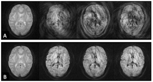
Diffusion-weighted EPI with (bottom row) and without parallel imaging (top row). (A) DWI scans on a patient suffering from multiple stroke lesions and hemorrhagic transformation. Without parallel imaging considerable pile-up artifacts are visible in the forebrain (arrows) as well as signal hyperintensities in the temporal lobes. Parallel imaging removes these confounding artifacts. (B) DWI on a patient with a coiled aneurism. Considerable metal artifacts can be seen on conventional EPI. Although not completely eliminated, parallel imaging (R=2 with partial L/R FOV of 75% effectively leading to 3-fold acceleration) could reduce the artifacts and reveal an ischemic lesion (open arrow).

Since fewer phase encode lines are acquired in parallel imaging, parallel imaging-enhanced scans come with a SNR penalty that is proportional to $\sqrt{\text{R}}$ plus an extra geometry-related factor⁴⁸, which depends on the number, size, and orientation of the individual receiver coils of the array relative to the prescribed FOV. Because of the geometry factor, or “g” factor, the SNR becomes spatially varying. Moreover, with increasing R the chances increase for residual aliasing artifacts and excessive local SNR enhancement. The extent to which this occurs depends on the individual design of the array coil. Some of the SNR penalty of parallel imaging enhanced diffusion-weighted EPI will be compensated by the shortened EPI train, which in turn affords a shorter echo time and less T₂-related signal loss⁵³. Due to EPI's fast acquisition capacity, the remaining SNR loss can be regained by adding extra averages. Of note here is that we have observed that parallel imaging enhanced DWI scans demonstrate much less T₂-shine through effect than regular DWI scans. On one hand this is advantageous to identify acute stroke lesions amongst pre-existing subacute lesions. On the other hand, subacute lesions become less conspicuous than with conventional EPI, but overall, in a recent study performed at our institution in 40 patients demonstrated a clear preference for the use of parallel imaging in concert with parallel imaging (Fig. 15).

Figure 15.

Comparison of resolution (128×128 vs. 192×192) and parallel imaging (R=1 vs. R=3) shown in a patient with multiple tiny infarctions. The higher spatial resolution and reduced distortion reduction using R = 3 was clearly preferred by three independent readers. Overall, 192×192 R=3 was the preferred option in all cases. Lesion conspicuity on the R=1 scans is generally higher for subacute infarcts because of TEs ∼80-90msec instead of ∼60msec for R=3 scans and the associated higher T₂-shine-through effect.

Parallel imaging reconstruction can be performed in the image domain (e.g. SENSE⁴⁸), in the k-space domain (e.g. GRAPPA⁴⁹), or in the hybrid domain (e.g. ARC^{54, 55}). Initially we started our parallel imaging efforts for DWI with SENSE, but lately our group switched to a hybrid domain approach⁵⁴, mainly because both the hybrid approach and GRAPPA have a more benign residual reconstruction artifacts, greater robustness against motion, and are more compatible with partial Fourier reconstruction⁵⁶. Initially, a variable-density k-space EPI sampling scheme was acquired to provide the intrinsic calibration information required for GRAPPA⁴⁹, with the region around the center of k-space sampled at the Nyquist sampling rate. However, as discussed in the previous section, geometric distortions in EPI depend on the v_ky. Thus, with a variable-density sampling scheme, different regions of k-space would contribute different amounts of distortions depending on their local v_ky. That is, around the center of k-space -- where data are sampled at the Nyquist rate (i.e. without any acceleration) -- a low spatial frequency image component with distortions equal to a normal EPI acquisition will be formed; whereas a high spatial frequency image component will be generated from the accelerated outer portion of k-space with considerably less distortions (Fig. 16). To avoid this artifact, it is beneficial to begin the DWI exam with a matching interleaved EPI scan (i.e. the number of interleaves should match R) and with the diffusion gradients turned off (b=0 sec/mm²), or use a calibration scheme as suggested by Newbould et al⁵⁷.

Figure 16.

(A) Single-shot EPI partial Fourier trajectory with variable-sampling density. The region around the center of k-space is sampled at the Nyquist rate. Due to the low k-space velocity, v_ky, equal to that of regular EPI no distortion reduction can be achieve for these spatial frequencies. (B) Corresponding EPI image. There is a misregistration between low-frequency image information content and the contour-determining high-spatial frequency components of the image due to the variable-density sampling and the resulting variable amount of distortions.

5.2. Phase Correction

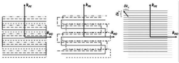
An inherent problem of single-shot EPI is the limited spatial resolution that can be achieved. Since all k-space data are acquired with a single readout train, T₂^*-related signal loss occurs. Thus, conventional EPI is typically performed with acquisition matrices up to 128×128 and at most 192×192 with the help of parallel imaging. Achieving higher spatial resolutions to become competitive with regular structural MRI requires to the use of multi-shot sequences. However, as discussed in section 2, multi-shot acquisitions bring back the problem of shot-to-shot phase variations caused by motion. In order to correct these phase variations, multi-shot sequences usually have to acquire additional navigator data from which these phase terms can be estimated for further correction of the imaging data. Such navigator data can be obtained from an extra navigator image prior to or after acquiring the imaging data (Fig. 13) or by using some specially designed readout trajectories that fully sample the center of the k-space at each acquisition, such as PROPELLER^58-60 or SNAILS³⁵ (Fig. 17). Typically, the navigator image is a low-resolution image that samples k-space at the Nyquist sampling rate or even higher. In the past, phase correction with the navigator images (as well as previous methods which used navigator projections in one^{61, 62} or two²⁸ dimensions) was performed in the k-space domain⁶³ instead of the preferred image domain; and this was only partially successful.

Figure 17.

Top: Long-axis PROPELLER (left), short-axis PROPELLER (center), and readout-segmented (right) trajectories. Bottom: constant-density spiral (left) and variable-density spiral (right). With long-axis PROPELLER (top, left) the frequency encode direction is along the long axis of the ‘blade’, whilst phase encoding is along the short-axis of the blade. With short-axis PROPELLER (top, center) and RS-EPI (top, right) the readout and phase encode axis are swapped so that the phase-encoding direction is along the long-axis of the blade. The variable-density spiral (bottom, right) samples the origin of k-space with greater density than peripheral portions of k-space. How quickly the spiral moves outward in radial direction is controlled by a pitch-factor variable.

Thus far, we have assumed that phase errors are only constant or linear in the image domain. However, as different regions within the FOV move most likely differently, the corresponding phase impressed on the spins following the diffusion preparation will be nonlinear in space. It is important to notice that even if there is just a linear phase variation impressed on the spins, when the readout method used is susceptible to geometric distortions (even to a lesser extent) this “phase tag” will be squeezed or stretched in the acquired image which effectively leads to an non-linear phase distribution in the resultant image⁶⁴. As a consequence: while a linear phase shift in the image domain causes a simple shift in k-space, a non-linear phase causes additional dispersion of the k-space data (Fig. 18). For an accurate correction of phase errors it is therefore important that the distortion properties of the navigator image match that of the multi-shot diffusion image. This is typically the case for most self-navigated trajectories, but can become somewhat difficult to achieve for trajectories that require an extra navigator image.

Figure 18.

Partial Fourier encoded k-space data (left) and corresponding images (right). The top row shows an EPI shot with typical quality, whilst the bottom row shows a poor quality shot with considerable k-space dispersion. Arrows indicate regions of profound signal distortions.

For self-navigating trajectories that allow one to reconstruct unaliased intermediate images acquired in each TR, such as PROPELLER⁵⁸, probably the simplest way to phase-correct DWI data is: (1) to appodize the high-spatial frequency components to get a low-pass filtered intermediate image that mostly contains the unwanted phase errors due to motion; (2) to multiply the original intermediate image by the complex conjugate of the low-pass filtered phase image. After this, the phase-corrected intermediate images can be combined (or gridded) in k-space, followed by an inverse FFT into the image domain to get the final diffusion-weighted image⁵⁹.

However, for a more generalized form of phase correction, which works on arbitrary k-space data, the non-linear phase correction proposed by Miller et al.⁶⁵ or the more elaborate version of Liu et al.^66-68 is recommended. The latter approach considers multi-channel coils, parallel imaging, off-resonances, and demonstrates a better SNR than the former approach. For interested readers we recommend an extention of Liu's approach by Aksoy et al.⁶⁹, which simultaneously corrects for subject movement between shots. Figure 19 (Phase correction demo) shows the performance of phase-correction on diffusion-weighted multi-shot data.

Figure 19.

(A) b=0 image and three b=900 sec/mm² images acquired with conventional spiral (constant density). The three diffusion gradient directions are: (0 1 -1)^T, (-1 1 0) ^T, and (0 1 1) ^T. (B) Images acquired with variable-density spiral. Non-linear phase correction was applied to both data sets. Clearly, the oversampling of the origin of k-space allows one to calculate a much better phase error estimate. Moreover, due to the central oversampling, the chances of violating the Nyquist criterion from k-space shifts are considerably lowered.

Even with navigator correction, with some trajectory types (e.g. interleaved EPI) one has to be careful with local violations of the Nyquist criterion (that is, regional undersampling of k-space). This is because the linear component of the image domain phase errors will shift the trajectories at arbitrary positions away from their desired positions in k-space (Fig. 6 and 19). To ameliorate this problem Atkinson et al.⁷⁰ recommended oversampling of k-space and signal averaging. This is another reason that makes the PROPELLER⁵⁸ trajectory very appealing, since the sampling within the PROPELLER-blade remains consistent. PROPELLER avoids many of these problems, as k-space shifts will affect the trajectory, similar to single-shot EPI, en bloc.

5.3. PROPELLER

The PROPELLER or Periodically Rotated Overlapping ParaLLEL Lines⁵⁸ technique has been introduced as a novel method that incorporates both 2D-navigation information with the benefits of a radial-type acquisition. This multi-shot technique covers a thin strip or “blade” of k-space with each acquisition (Fig. 17). As discussed in more detail later, by phase cycling the RF refocusing pulses, the FSE train is stabilized and avoids phase errors that lead to a violation of the MG condition.

PROPELLER's inherent oversampling near the origin of k-space allows the removal of blades that contain uncorrectable errors from motion during diffusion-encoding, such as excessive through-plane dephasing or k-space shifts that move the center of k-space outside the sampling of the blade. Because of the radial-type acquisition of this trajectory and the redundant sampling around the origin, the missing k-space data in the peripheral k-space regions will cause only some benign streaking artifacts⁷¹.

FSE-based PROPELLER DWI has been demonstrated to be very useful in areas with severe susceptibility distortions where EPI suffers from strong image degradation, such as areas close the base of the skull or metallic material⁵⁹, or when higher spatial resolution is needed. Like other multi-shot techniques, the scan time of PROPELLER (which is exacerbated by excessive k-space oversampling, the FSE RF pulses and gradient balancing) is substantially longer than conventional single-shot EPI. This may limit PROPELLER's utility in acute stroke or for breath-hold studies where scan time is critical. Due to the requirement of relatively large flip angles to cope with the non-MG issues, diffusion-weighted FSE PROPELLER becomes particularly SAR-intense and dependent on homogeneous RF transmission fields. All of that is less problematic at 1.5T, but can be challenging at 3T. To reduce SAR and boost scan efficiency, Pipe et al.⁷² recently introduced the turboPROP method, which is based on a GRASE⁷³ readout rather than a conventional FSE train. In GRASE, more than one gradient echo is acquired between two subsequent refocusing pulses in the FSE train and, thus, will speed up the readout whilst using fewer SAR-intense refocusing pulses. TurboPROP provides a good tradeoff between fast data acquisition schemes, such as EPI, and low-distortion acquisition methods, such as FSE, as was demonstrated recently for fiber tracking applications by Arfanakis et al⁷⁴.

5.4. Short-Axis (Readout) PROPELLER EPI

Skare et al.⁶⁰ leveraged on the great navigation capability and k-space data consistency of individual blades of the PROPELLER trajectory and paired it with the minimum-SAR and short scan time features of EPI. Here, the dimensions of the trajectory were transposed relative to the original PROPELLER trajectory (Fig. 17). This serves to accelerate the traversal through k-space and thus reduce EPI-related distortions. Rather than using the long axis of the PROPELLER blade for the readout, the readout was placed along the short axis of the PROPELLER blade (with the phase-encoding along the long axis). For a 256×256 acquisition matrix using 32×256 blades, a theoretical 8-fold reduction of EPI-related distortions can be achieved, which can be further diminished by parallel imaging (additional ∼3-fold reduction) and by distortion correction post-processing methods using the B0-field map obtained from reversed gradient polarity methods⁴². Note that transposing the PROPELLER axes is crucial to benefit from the distortion reduction capability of the short-axis readout PROPELLER blade⁶⁰. If the long-axis PROPELLER version is used in concert with EPI^{75, 76} there is no geometric distortion benefit over conventional Cartesian EPI. In fact, due to the radial nature of PROPELLER, EPI distortions will be smeared radially, causing blurring in the final image. This can be illustrated in Figure 20, showing a comparison between short-axis and long-axis PROPELLER EPI. In addition to CNS studies, diffusion-weighted PROPELLER FSE^77-79 has recently been applied to abdominal imaging. Adding moderate diffusion attenuation helps to reduce the high signal from vessels in the liver and improve lesion conspicuity. As shown in Fig. 21, the rapid imaging capacity of short-axis PROPELLER EPI makes the sequence well suited for breath-hold studies, and has potential for DWIBS (c.f. section 7.2).

Figure 20.

Comparison of single-shot EPI (top, left), with long-axis PROPELLER EPI (top, right) and short-axis PROPELLER EPI (bottom, left). All blades were 32×256 (short axis PROPELLER = SAP) and 256=32 (long axis PROPELLER = LAP). Distortions with SAP EPI are markedly reduced. For each method, 25 blades were used and were swept over a range between 0 and 180 degrees. For reference, a matching T₂w-FSE is shown as well (bottom, right).

Figure 21.

Short Axis PROPELLER EPI of the abdomen with 30 8mm slices (1mm gap) using 10 64×256 blades with b=500 sec/mm². (A) Non-breathhold acquisition showing three isotropic DWI (left) and mean ADC (right) images located 18mm apart; (B) breathhold acquisition; (C) corresponding free-breathing FSE acquisition.

5.5. Readout-Segmented EPI (RS-EPI)

In the previous section we have seen that reading out echoes with a length only a fraction of that of the nominal readout resolution shortens the echo spacing dramatically and allows one to traverse k-space much faster. In this fashion, artifacts can be significantly reduced but require multiple shots to fully cover the entire k-space. One way to cover k-space was the short-axis EPI PROPELLER approach. Alternatively, one can shift the blades along the readout dimension without rotating the blade⁸⁰. When combined with diffusion-weighting, an additional navigator image needs to be acquired^{81, 82} since every blade no longer goes through the center of k-space. Typically, this can be done by adding another 180° refocusing pulse and an additional short-axis readout located at the center of k-space^{83, 84}. A similar phase correction as discussed in section 5.1 can be used, except that the phase-reversal of the extra 180° refocusing pulse must be considered. Again, parallel imaging can be used to further reduce distortions^{83, 84}. Compared to the short-axis readout PROPELLER EPI version, the need for extra navigator data cuts down slightly on scan efficiency and the overlapped sampling of central regions of k-space also leaves PROPELLER with an SNR advantage over the RS-EPI version given the right choice of scan parameters⁸⁵. However, the overlapping causes structural image noise (i.e., non-white noise), which essentially lowers the effective resolution of any PROPELLER method. Lastly, since motion can be detected from the navigator image as well, RS-EPI is also well suited to correct for motion (Fig. 22).

Figure 22.

Diffusion-weighted RS-EPI in the presence of moderate (top) and severe (bottom) patient motion. Before (middle column) and after (right column) motion correction. (top, left) Reference image, for which the volunteer was asked to remain stationary.

5.6. Spirals

A few studies have recently explored the self-navigating capability of the spiral readout trajectory in multi-shot DWI^{34-36, 86}. Previously, magnetic resonance imaging (MRI) based on spiral readout (Fig. 17) has been found effective in applications such as functional neuroimaging^{87, 88} and spectroscopy^89-92. The spiral trajectory has the merit of moment-nulling motion compensation and efficient use of gradient power³³. However, it turns out that conventional (constant density) spiral readout trajectories have limited potential for self-navigation because of the lack of data in the central k-space. This effectively allows zero- and (to some extent) first-order compensation only⁶³. In order to improve the navigating capability, one can increase the sampling density at the center of the k-space. With a recently developed analytic variable-density spiral design technique⁸⁹, the k-space sampling density can easily be increased around the origin of k-space. This leads to a diffusion-weighted multi-shot variable-density spiral sequence design, which is a self-navigated technique and a promising alternative for high resolution DWI³⁵. With the analytic variable-density spiral design technique, the k-space sampling density can be easily manipulated and prescribed on the scanner hardware in real time. Here, each spiral interleaf oversamples the central region of the k-space and undersamples the outer region of the k-space (Fig. 17). The sampling density is circularly symmetric and decreases smoothly as the radius increases in k-space. For each spiral interleaf, the phase error in image space can be estimated from the fully sampled center of k-space, and used for subsequent phase correction^{35, 69, 93}. Compared to constant density spirals the image quality is improved dramatically with variable-density spirals. Oversampling the origin of k-space also helps to reduce the aforementioned artifacts from the linear phase error terms that lead to local undersampling of k-space (Fig. 19).

6. Coping with the Non-MG Component in FSE

6.1. Phase Cycling

For their original diffusion-weighted PROPELLER FSE work Pipe et al.⁵⁹ suggested mitigating signal instability present in FSE-based DWI by varying the phase of the refocusing pulses between the x- and y-axes, i.e. 180°_x - 180°_y - 180°_x - 180°_y and so forth, in the fashion of well-known phase cycling schemes^94-96. This produces a relatively stable echo train for refocusing angles near 180°, but the echo amplitudes begin to fall off significantly for refocusing angles down to 140° (Fig. 23). Although robust in general, this approach can be problematic in the presence of poor slice profiles (i.e. when the transition band is a large fraction of the overall slice thickness) or at higher magnetic field strengths where more non-uniform transmit RF fields occur in the presence of B1 inhomogeneities from dielectric effects. The requirement to keep the refocusing angles well above 140° might become problematic for high-field applications due primarily to SAR concerns. However, methods such as VERSE⁹⁷ or TurboPROP⁷² have been suggested to lower SAR.

Figure 23.

Bloch simulations of multi-echo readout with spin phase 0° (black=CPMG component), 30° (red), 60° (green), and 90° (blue=non-CPMG component) relative to RF axis of the FSE train. Relaxation effects were neglected. The flip angle for all refocusing pulses was reduced from 180° to 150°. (A) The RF phase remained constant over the FSE train. This results in considerable signal loss and oscillations of the individual echoes of the FSE train if the phase of the transverse magnetization deviates from the MG phase condition. (B) With XY phase cycling oscillates slightly but the signal amplitude remains independent from the initial phase of the transverse magnetization.

A very similar approach to that of Pipe et al. has been introduced recently by Le Roux³¹. It differs by being able to sustain echo trains for a larger number of echoes and allowing for a larger acceptable non-uniformity of the transmit RF (that is, variations down to an effective refocusing flip angles of 115°³¹). Unlike Pipe's XY phase cycling approach, Le Roux suggests a quadratic phase modulation scheme⁹⁵ in order to set the RF phase of the refocusing pulses within the FSE train.

6.2. Elimination of the non-MG component

Norris et al.⁹⁸ have shown that for a CPMG train, the echoes formed by magnetization that has spent an odd number of inter-refocusing pulse periods in the transverse plane add coherently to form a single odd-parity echo, whilst an even-parity echo forms analogously. Moreover, they belong to two separate echo families: (1) family A, that occurring simultaneously with the repeated direct refocusing of the first spin-echo A₁; (2) family B, that occurring simultaneously with the direct refocusing of the first stimulated-echo B₁. Refocusing flip angles differing from pure 180° will lead to an intermingling of the two families. The odd and even echoes in each acquisition period come alternatively from the A and B families. By creating a significant enough imbalance between the readout dephaser gradient and the readout gradient (that is, the dephaser gradient area is considerably different from half of the readout gradient area), Norris et al.⁹⁸ achieved that the two echo parities occur temporally disseminated in the readout window (Fig. 24). With this method, also known as displaced U-FLARE, one echo parity (typically the odd one) is pushed out of the window when each echo is acquired at the price of half the available signal-to-noise ratio (SNR) and the need for several dummy echoes to stabilize the signal in the FSE train. Recently, Norris⁹⁹ improved his original approach by means of selective parity imaging. Again, displacing gradients were used, but – in contrast to displaced U-FLARE – both odd and even parity echoes were selected within a single echo train whereby the echo parity was chosen that gave the desired signal strength at the lowest refocusing angle. Furthermore, the first echo was an 180° refocusing pulse to boost signal amplitude and a central-out phase encoding scheme was used to minimize TE. Lastly, a recursive application of the Bloch equations was used to generate a smooth signal decay over the FSE train to minimize image blurring.

Figure 24.

U-FLARE sequence with imbalanced dephasing and readout gradients (shaded area) as originally suggested by Norris et al. The graph shows the formation of the echoes for the first three cycles of an FSE train using these imbalanced gradients. Here, the readout dephasing gradient area is too big as shown by the gray area. This generates two echo families A and B. The odd (red) and even (blue) parities are made up by both families as shown in the figure. In the original displaced U-FLARE approach the gradient imbalance was made that strong so that one of the echo parities was pushed outside the sampling window.

Alsop¹⁰⁰ introduced a preparation method for non-CPMG FSE (again at the cost of half the signal) in which a dephasing gradient followed by a 90° was applied prior to the FSE train. By applying a dephasing gradient prior to the formation of the diffusion-weighted spin-echo he achieved so that each voxel has equal components of MG and non-MG signal. The 90° echo-reset pulse – played out along along the same axis as the subsequent FSE pulses – will rotate the non-MG component to the longitudinal axis where it will be invisible in the subsequent sequence (Fig. 25). In addition, rephasing gradients of opposite polarity (but with identical gradient area as the dephaser gradient), must be added following each refocusing pulse and before the acquisition of each echo, and then rewound after each acquisition and prior to the next refocusing pulse to maintain the MG condition. To permit acquisition of data from the very first echo without artifact, Alsop ramped down the flip angles of the FSE train from 142.2° to 94.9°, 69.2°, and 63.0°and with remaining pulses set to 60°.

Figure 25.

Diffusion-weighted fast spin-echo sequence as suggested by Alsop. Prior to t=TE a dephasing gradient is applied (solid fill) that distributes the spins evenly in the transverse plane into MG and non-MG components. The non-MG component is then aligned longitudinally by an echo reset pulse at t=TE. For each echo readout the dephasing of the MG component must be first undone and reapplied after echo sampling.

7. Outside the Box

7.1. Diffusion-weighted SSFP

3D imaging is extremely cumbersome with conventional spin-echo Stejskal-Tanner sequences because the long TEs and TRs render conventional DWI sequence prohibitively long. An alterative technique that allows rapid image formation suitable for 3D imaging is steady-state free precession (SSFP). In SSFP, a train of equidistant RF pulses with flip angle α and TR<T₂ is applied, and a condition of steady-state free precession develops after a few TRs. SSFP imaging is also known for its high sensitivity to flow and diffusion in the presence of magnetic field gradients¹⁰¹. Together with its 3D imaging capibilities, diffusion-weighted SSFP is therefore an attractive alternative to conventional DWI.

By adding a single, short diffusion gradient within the TR interval between successive RF pulses and before the gradient echo readout, the diffusion sensitivity of the sequence can be boosted (Fig. 26). SSFP has therefore gotten attention from several researchers^{93, 102-104}. In contrast to the commonly used Stejskal-Tanner preparation, the signal formation in SSFP is a complex superposition of numerous spin and stimulated echoes, each of which may be formed through a multitude of coherence pathways^{105, 106}, limited only by the natural decay times T₁ and T₂. Contributions from any of these coherence pathways to an echo might have experienced various amounts of diffusion encoding gradients and may have spent more or less time stored as longitudinal (T₁ decay) or transverse (T₂ decay) magnetization. This complex signal formation renders the quantification of diffusion-weighted SSFP very difficult, and diffusion weighted SSFP methods are currently mostly limited to qualitative applications. Thus, the diffusion attenuation (b-factor) may vary from tissue to tissue. In contrast to Stejskal-Tanner DWI sequences, one therefore has to deal not only with “T₂-shine-trough” effects but also with the fact that b-values are weighted by the underlying relaxation times and other confounding factors. Recently, McNab et al.¹⁰⁷ have introduced a formalism to describe the contribution from relaxation and flip angle to the diffusion-weighted SSFP signal and assessed their contributions. This is a promising step, and potentially opens a viable avenue for 3D diffusion imaging – a technique much sought after, especially for DTI and associated fiber tracking methods.

Figure 26.

One cycle of a diffusion-weighted SSFP sequence: The ECHO component is generally very sensitive to diffusion. Except for the diffusion-encoding gradient all other gradients are completely balanced and the total effective gradient is equal in each cycle to establish a steady state.

7.2. DWIBS

The low ADC of lymph nodes and their metastatic infiltrates as well as that of many malignant primary tumors have recently led to an increased interest in using DWI for diffusion-weighted whole body imaging with background body signal suppression (DWIBS)^{5, 108, 109}. DWIBS has received a lot of acclaim and has caused considerable excitement in the community as it has become an important contributor to the diagnostic value of whole-body MRI, which in turn has become a serious competitor for both PET and PET-CT^110-112.

Different variants of DWIBS exist, but the basic idea is common to all of them: First, low ADC lipids are suppressed; second, DWI of either the entire body or a region of interest is performed with considerable (for tissue outside the CNS) diffusion attenuation to make the low ADC structures stand out (e.g. 500-1000 sec/mm²), while the remainder of the other tissues are suppressed; third, maximum intensity projections (MIPs) are computed at different projection angles to improve lesion visibility and facilitate diagnostic utility; fourth, an inverted gray scale is applied to the MIPs. That is, low ADC structures will appear hypointense, whereas regular background appears bright to resemble scintigraphic images. The latter step is cosmetic and can be used depending on the preference of the interpreting radiologist.

DWIBS offers images that are similar in appearance to PET, but the diagnostic potential of DWIBS awaits head to head comparison in large patient cohorts. When using DWIBS for the staging of lymphoma patients, DWIBS may aid in the detection of lymph nodes. However, after detection, additional judgment is still required, using morphological criteria, such as size and shape of the lymph nodes. Particularly for lymph nodes it remains to be seen whether DWIBS can be of use in discriminating benign from malignant nodes.

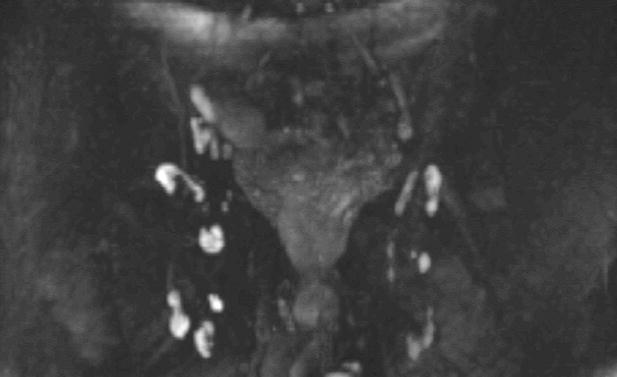
Figure 27 demonstrates DWIBS performed on a patient suffering from a lymphoma. The widespread disease is clearly visible on this coronal MIP. For whole-body applications and/or adipose patients with large girth sizes, achieving fat suppression based on frequency selective methods (e.g. CHESS, spectral-inversion recovery (SPIR), spectral-spatial excitation) often fails because of the homogeneity of the magnet across such a large FOV. This leaves regions of incompletely suppressed, and low-ADC fat behind that will appear hyperintense on DWIBS and will impair automatic MIP processing. While incomplete fat-suppression is not problematic for most sequences, the very low ADC makes even small fractions of remaining fat stand out on the MIPs. STIR-based nulling of lipids has been suggested⁵. However, the penalty of using STIR is a considerable SNR loss, since all other tissue is also inverted and only partially recovered at TIs of ∼160-200msec. Moreover, at 3T, STIR can be somewhat challenging (even with adiabatic inversion pulses), and – at least on our system – has occasionally failed to null fat entirely. Furthermore, the STIR preparation decreases the scan efficiency considerably.

Figure 27.

Female patient suffering from lymphoma. The whole-body DWIBS exam (A) clearly reveals numerous disseminated lesions throughout the body. In the right hip region the CHESS fat suppression failed to work. (B) corresponding whole-body T₁w FSE. Patient raw data set courtesy of Dr. R.A.J. Nievelstein and T.C. Kwee, UMC Utrecht, the Netherlands.

In situations when fat suppression fails, cut-out MIPs are a good option (Fig. 28). In our experience, cut-out MIPs of smaller areas can better reveal abnormalities and are less affected by surrounding clutter. The benefit of cut-out MIPs is well known from MRA and can often be useful (personal communication, Dr. Houston, Mayo Clinic). However, when only crude cut out-MIPs are used superficial lymph nodes, in the example in Fig. 28 the inguinal lymph nodes, are cut off, which – if only reviewing the MIP – is easily overlooked. Another problem is also that the bright fatty layers are often on the ventral AND lateral side of a patient, i.e.: if the patient were a cube, the bright fat is on two faces of the cube, making it nearly imposible to ‘look behind it’ even by rotating the volume MIP. If fat-suppression fails only on 1 side “of the cube” it is just aesthetically less pleasing, but less of a clinical problem, because rotating the MIP will allow a reader to look “behind” the superimposing bright fat. An easier solution is the use of thin-slab MIPs (Fig. 28c and d), although as shown in our example, caution must also be exercised, and as with MRA, the thin source images should always be reviewed.

Figure 28.

One station from the multi-station whole-body exam shown in Fig. 27 where fat suppression on the patients right side was incomplete. Due to the low-ADC of fat it appears hyperintense on DWI scans and thus affecting the MIP procedure (A). Some of the diseased lymphatic tissue is poorly visualized on the MIP. A crude cut-out MIP (B) can get rid of some of the fat but is still not fully satisfying. Ideally 3D shaped cut-outs offered by some advanced image processing workstations would better suited. (C) Thinner slab MIPs helps to reveal the lymph nodes in the abdomen (arrows), but the inguinal nodes were outside of the slab and missed. Changing the slab location (D) will bring back those nodes but unsuppressed fat come back in the abdominal region, masking nodes. This example demonstrates the importance of good fat suppression and/or the availability of cut-out MIP tools.

It is also our experience that for certain regions, conventional fat suppression works equally well (as can be seen from Fig. 27). This, of course, has a tremendous advantage as it boosts scan performance (i.e. more slices per TR) and SNR. Without the concern about fat suppression and consequently reduced SNR, one can focus on resolution and thinner sections. Figure 29 shows an example of such a study on a male pelvis, which clearly reveals the morphologic structure of inguinal lymph nodes in much better detail. However, as mentioned before, the readout time for conventional single-shot EPI lengthens with increasing resolution - to the point that blurring and geometric distortions impair image acquisition. Parallel imaging ameliorates this problem to some extent, but for certain applications, such as (sentinel) node screening in the axilla, the coil sensitivity variation and coverage provided by the coil elements are suboptimal and parallel imaging soon reaches its limits. At our institution we have therefore switched to multi-shot techniques, such as SNAILS³⁵. Figure 30 shows a comparative evaluation of SNAILS together with single-shot EPI with and without parallel imaging, demonstrating the potential superiority of multi-shot scans for DWIBS.

Figure 29.

Thin section (3mm/0mm gap) DWIBS of the male pelvis (without grayscale inversion) using spectral-spatial water-only excitation. The inguinal lymph nodes and their morpholgic structure are well visualized.

Figure 30.

High-resolution DWI of the breast and axillary lymph nodes. (A). 256×256 DW-EPI is severely distorted despite the use of parallel imaging (ASSET); (B) 128×128 ASSET-DW-EPI; (C) 256×256 Multi-shot SNAILS-DWI reveals much better details and is less distorted. High-resolution SNAILS data set allows multiplanar reformats for DWIBS processing and show clearly axillary lymph nodes on both unilateral sagittal MIP (D) and coronal chest-wall MIP (E). The SNAILS acquisition time was 5min for both breasts and axillas.

Very often the use of multi-shot scans makes the scan duration of DWIBS prohibitively long, especially in abdominal scans when breath holds are warranted to limit motion artifacts. While free breathing is typically tolerable in the pelvis, respiratory motion in the abdomen is too severe to allow free breathing. Alternatively, respiratory gating can be used but – again -- leads to a considerable prolongation of the entire DWIBS exam. A possible alternative is the recently introduced tracking-only navigator (TRON) technique¹¹³. This technique does not use the navigator for gating image acquisition but for the tracking of movement. The tracking data is then retrospectively used to correct for displacement of structures, as for example caused by breathing motion. The technique only corrects for linear displacement of sub-diaphragmatic tissues. For relatively small structures, such as lymph nodes, this is probably fine. For larger structures such as the liver, which not only translate but also deform during respiratory motion, this remains to be investigated. Nevertheless, the first data indicate that TRON may improve image quality of DWIBS, with a minimal prolongation of acquisition time.

Aside from being sensitive to lymph nodes, DWIBS turned out to reveal nerve fibers and paraspinal ganglions very well. However, DWIBS is nothing else other than a regular DWI sequence, and therefore is sensitive to anisotropic diffusion (Fig. 31). The ability to perform neurographic imaging outside the CNS has been done with DTI for the median nerve before, but recently DWIBS was also used to examine the brachial¹¹⁴ and the lumbosacral plexus¹¹⁵. The main advantage of using DWIBS again is in the suppression of background detail. This is especially beneficial to neurography because DWI can suppress the signal from bloodvessels, which often course alongside nerves in neurovascular bundles. Suppresion of background also allows MIP visualization of the often complex anatomy of a nerve plexus and aids in for example the discrimination of primary neuronal diseases, such as tumors, from extra-neuronal pathology compressing or infiltrating the plexus.

Figure 31.

(A) Visualization of the lumbar nerves in a patient (arrowheads) using DWIBS (without inverted gray scale). (B) DWIBS in another patient clearly reveals the spinal cord as well as the nerve roots and ganglions (arrows). (gb … gall bladder, s … spleen, rk … right kidney, lk … left kidney).

9. Conclusion

Fifteen years ago DWI was performed mostly on systems with special gradient hardware or insert gradients and with limited EPI upgrades, which provided only few isolated institutions with the access to DWI. Advances in MR scanner hardware over the last decade (such as high-performance gradient coils, better magnet homogeneity, and multi-channel coils that facilitate parallel imaging) made EPI and DWI much more accessible to a broader user base. Nowadays, diffusion-weighted EPI belongs to the key sequences of a clinical MR system and DTI has been used in hundreds of research studies.

This article described the major salient problems that still remain with DWI and potential solutions for solving these problems. After many years of struggling with mediocre image resolution and distortions, some of the solutions presented here offer possibilities to achieve DWI with image quality comparable to conventional structural imaging; something probably unthinkable ten years ago. The purpose of this article was also to provide the radiologist with an overview about the strengths and weaknesses of current DWI methods.

References

- 1.Moseley ME, Cohen Y, Mintorovitch J, Chileuitt L, Shimizu H, Kucharczyk J, Wendland MF, Weinstein PR. Early detection of regional cerebral ischemia in cats: Comparison of diffusion- and t2-weighted mri and spectroscopy. Magn Reson Med. 1990;14:330–346. doi: 10.1002/mrm.1910140218. [DOI] [PubMed] [Google Scholar]
- 2.Albers GW, Lansberg MG, O'Brien MW, Ali J, Woolfenden AR, Tong DC, Moseley ME. Evolution of cerebral infarct volume assessed by diffusion-weighted mri: Implications for acute stroke trials. Neurology. 1999;52:A453. [Google Scholar]
- 3.Callaghan PT, Coy A, MacGowan D, Packer KJ, Zelaya FO. Diffraction-like effects in nmr diffusion studies of fluids in porous solids. Nature. 1991;351:467–469. [Google Scholar]
- 4.Basser PJ, Mattiello J, LeBihan D. Estimation of the effective self-diffusion tensor from the nmr spin-echo. J Magn Reson B. 1994;103:247–254. doi: 10.1006/jmrb.1994.1037. [DOI] [PubMed] [Google Scholar]
- 5.Takahara T, Imai Y, Yamashita T, Yasuda S, Nasu S, Van Cauteren M. Diffusion weighted whole body imaging with background body signal suppression (dwibs): Technical improvement using free breathing, stir and high resolution 3d display. Radiat Med. 2004;22:275–282. [PubMed] [Google Scholar]
- 6.Torrey HC. Bloch equations with diffusion terms. Phys Rev. 1956;104:563–565. [Google Scholar]
- 7.Stejskal EO, Tanner JE. Spin diffusion measurements: Spin echoSpin-echoes in the presence of a time-dependent field gradient. J Chem Phys. 1965;42:288–292. [Google Scholar]
- 8.Basser PJ. Inferring microstructural features and the physiological state of tissues from diffusion-weighted images. NMR Biomed. 1995;8:333–344. doi: 10.1002/nbm.1940080707. [DOI] [PubMed] [Google Scholar]
- 9.Jones DK, Horsfield MA, Simmons A. Optimal strategies for measuring diffusion in anisotropic systems by magnetic resonance imaging. Magn Reson Med. 1999;42:515–525. [PubMed] [Google Scholar]
- 10.Fliege J, Maier U. The distribution of points on the sphere and corresponding cubature formulae. IMA J NUMER ANAL. 1999;19:317–334. [Google Scholar]
- 11.Skare S, Hedehus M, Moseley ME, Li TQ. Condition number as a measure of noise performance of diffusion tensor data acquisition schemes with mri. J Magn Reson. 2000;147:340–352. doi: 10.1006/jmre.2000.2209. [DOI] [PubMed] [Google Scholar]
- 12.Basser PJ, Pajevic S, Pierpaoli C, Duda J, Aldroubi A. In vivo fiber tractography using dt-mri data. Magn Reson Med. 2000;44:625–632. doi: 10.1002/1522-2594(200010)44:4<625::aid-mrm17>3.0.co;2-o. [DOI] [PubMed] [Google Scholar]
- 13.Mori S, Crain BJ, Chacko VP, van Zijl PC. Three-dimensional tracking of axonal projections in the brain by magnetic resonance imaging. Ann Neurol. 1999;45:265–269. doi: 10.1002/1531-8249(199902)45:2<265::aid-ana21>3.0.co;2-3. [DOI] [PubMed] [Google Scholar]
- 14.Frank LR. Anisotropy in high angular resolution diffusion-weighted mri. Magn Reson Med. 2001;45:935–939. doi: 10.1002/mrm.1125. [DOI] [PubMed] [Google Scholar]
- 15.Frank LR. Characterization of anisotropy in high angular resolution diffusion-weighted mri. Magn Reson Med. 2002;47:1083–1099. doi: 10.1002/mrm.10156. [DOI] [PubMed] [Google Scholar]
- 16.Callaghan PT. Principles of nuclear magnetic resonance microscopy. Oxford: Clarendon Press; 1993. [Google Scholar]
- 17.Assaf Y, Cohen Y. Structural information in neuronal tissue as revealed by q-space diffusion nmr spectroscopy of metabolites in bovine optic nerve. NMR Biomed. 1999;12:335–344. doi: 10.1002/(sici)1099-1492(199910)12:6<335::aid-nbm581>3.0.co;2-a. [DOI] [PubMed] [Google Scholar]
- 18.Assaf Y, Ben-Bashat D, Chapman J, Peled S, Biton IE, Kafri M, Segev Y, Hendler T, Korczyn AD, Graif M, Cohen Y. High b-value q-space analyzed diffusion-weighted mri: Application to multiple sclerosis. Magn Reson Med. 2002;47:115–126. doi: 10.1002/mrm.10040. [DOI] [PubMed] [Google Scholar]
- 19.Wedeen VJ, Wang RP, Schmahmann JD, Benner T, Tseng WY, Dai G, Pandya DN, Hagmann P, D'Arceuil H, de Crespigny AJ. Diffusion spectrum magnetic resonance imaging (dsi) tractography of crossing fibers. Neuroimage. 2008;41:1267–1277. doi: 10.1016/j.neuroimage.2008.03.036. [DOI] [PubMed] [Google Scholar]
- 20.Wedeen VJ, Hagmann P, Tseng WY, Reese TG, Weisskoff RM. Mapping complex tissue architecture with diffusion spectrum magnetic resonance imaging. Magn Reson Med. 2005;54:1377–1386. doi: 10.1002/mrm.20642. [DOI] [PubMed] [Google Scholar]
- 21.Tuch DS. Q-ball imaging. Magn Reson Med. 2004;52:1358–1372. doi: 10.1002/mrm.20279. [DOI] [PubMed] [Google Scholar]
- 22.Liu C, Bammer R, Acar B, Moseley ME. Characterizing non-gaussian diffusion by using generalized diffusion tensors. Magnetic Resonance in Medicine. 2004;51(5):924–937. doi: 10.1002/mrm.20071. [DOI] [PubMed] [Google Scholar]
- 23.Skare S, Andersson JL. On the effects of gating in diffusion imaging of the brain using single shot epi. Magn Reson Imaging. 2001;19:1125–1128. doi: 10.1016/s0730-725x(01)00415-5. [DOI] [PubMed] [Google Scholar]
- 24.Poncelet BP, Wedeen VJ, Weisskoff RM, Cohen MS. Brain parenchyma motion: Measurement with cine echo-planar mr imaging. Radiology. 1992;185:645–651. doi: 10.1148/radiology.185.3.1438740. [DOI] [PubMed] [Google Scholar]
- 25.Chow LC, Bammer R, Moseley ME, Sommer FG. Single breath-hold diffusion-weighted imaging of the abdomen. J Magn Reson Imaging. 2003;18:377–382. doi: 10.1002/jmri.10353. [DOI] [PubMed] [Google Scholar]
- 26.Chow LC, Chang R, Bammer R. Diffusion weighted imaging in the assessment of renal dysfunction. 12th Annual Meeting of the ISMRM; 2004. p. 567. [Google Scholar]
- 27.Anderson AW, Gore JC. Analysis and correction of motion artifacts in diffusion weighted imaging. Magn Reson Med. 1994;32:379–387. doi: 10.1002/mrm.1910320313. [DOI] [PubMed] [Google Scholar]
- 28.Butts K, de Crespigny A, Pauly JM, Moseley M. Diffusion-weighted interleaved echo-planar imaging with a pair of orthogonal navigator echoes. Magn Reson Med. 1996;35:763–770. doi: 10.1002/mrm.1910350518. [DOI] [PubMed] [Google Scholar]
- 29.Meiboom S, Gill D. Modified spin-echo method for measuring nuclear relaxation times. Rev Sci Instr. 1958;29:688–691. [Google Scholar]
- 30.Poon CS, Henkelman RM. Practical t2 quantitation for clinical applications. J Magn Reson Imaging. 1992;2:541–553. doi: 10.1002/jmri.1880020512. [DOI] [PubMed] [Google Scholar]
- 31.Le Roux P. Non-cpmg fast spin-echo with full signal. J Magn Reson. 2002;155:278–292. doi: 10.1006/jmre.2002.2523. [DOI] [PubMed] [Google Scholar]
- 32.Mansfield P. Multi-planar image formation using nmr spin-echoes. J Phys C. 1977;10:L55–L58. [Google Scholar]
- 33.Glover GH. Basic and advanced concepts of spiral imaging. ISMRM Fast MRI Workshop. 1997:115–119. [Google Scholar]
- 34.Li TQ, Takahashi AM, Hindmarsh T, Moseley ME. Adc mapping by means of a single-shot spiral mri technique with application in acute cerebral ischemia. Magn Reson Med. 1999;41:143–147. doi: 10.1002/(sici)1522-2594(199901)41:1<143::aid-mrm20>3.0.co;2-o. [DOI] [PubMed] [Google Scholar]
- 35.Liu C, Bammer R, Kim DH, Moseley ME. Self-navigated interleaved spiral (snails): Application to high-resolution diffusion tensor imaging. Magnetic Resonance in Medicine. 2004;52(6):1388–1396. doi: 10.1002/mrm.20288. [DOI] [PubMed] [Google Scholar]
- 36.Bammer R, Glover GH, Moseley ME. Diffusion tensor spiral imaging. 10th Annual Meeting ot the International Society of Magnetic Resonance in Medicine; 2002. p. 1111. [Google Scholar]
- 37.Liu C, Bammer R, Acar B, Moseley ME. Generalized diffusion tensor imaging (gdti) using higher order tensor (hot) statistics. Magn Reson Med. 2004;51:924–937. doi: 10.1002/mrm.20071. [DOI] [PubMed] [Google Scholar]
- 38.Ozarslan E, Mareci TH. Generalized diffusion tensor imaging and analytical relationships between diffusion tensor imaging and high angular resolution diffusion imaging. Magn Reson Med. 2003;50:955–965. doi: 10.1002/mrm.10596. [DOI] [PubMed] [Google Scholar]
- 39.Ozarslan E, Shepherd TM, Vemuri BC, Blackband SJ, Mareci TH. Fast orientation mapping from hardi. Med Image Comput Comput Assist Interv Int Conf Med Image Comput Comput Assist Interv. 2005;8:156–163. doi: 10.1007/11566465_20. [DOI] [PubMed] [Google Scholar]
- 40.Tuch DS, Reese TG, Wiegell MR, Makris N, Belliveau JW, Wedeen VJ. High angular resolution diffusion imaging reveals intravoxel white matter fiber heterogeneity. Magnetic Resonance in Medicine. 2002;48(4):577–582. doi: 10.1002/mrm.10268. [DOI] [PubMed] [Google Scholar]
- 41.Farzaneh F, Riederer SJ, Pelc NJ. Analysis of t2 limitations and off-resonance effects on spatial resolution and artifacts in echo-planar imaging. Magn Reson Med. 1990;14:123–139. doi: 10.1002/mrm.1910140112. [DOI] [PubMed] [Google Scholar]
- 42.Chang H, Fitzpatrick JM. A technique for accurate magnetic resonance imaging in the presence of field inhomogeneities. IEEE Trans Med Imag. 1992;11:319–329. doi: 10.1109/42.158935. [DOI] [PubMed] [Google Scholar]
- 43.Andersson JL, Skare S, Ashburner J Karolinska Mr Research Centre SSjaks. How to correct susceptibility distortions in spin-echo echo-planar images: Application to diffusion tensor imaging. NeuroImage. 2003;20(2):870–888. doi: 10.1016/S1053-8119(03)00336-7. [DOI] [PubMed] [Google Scholar]
- 44.Reese TG, Heid O, Weisskoff RM, Wedeen VJ. Reduction of eddy-current-induced distortion in diffusion mri using a twice-refocused spin-echo. Magn Reson Med. 2003;49:177–182. doi: 10.1002/mrm.10308. [DOI] [PubMed] [Google Scholar]
- 45.Bammer R, Auer M. Correction of eddy-current induced image warping in diffusion-weighted single-shot epi using constrained non-rigid mutual information image registration. 2001:508. [Google Scholar]
- 46.Andersson JL, Skare S. A model-based method for retrospective correction of geometric distortions in diffusion-weighted epi. Neuroimage. 2002;16:177–199. doi: 10.1006/nimg.2001.1039. [DOI] [PubMed] [Google Scholar]
- 47.Haselgrove JC, Moore JR. Correction for distortion of echo-planar images used to calculate the apparent diffusion coefficient. Magn Reson Med. 1996;36:960–964. doi: 10.1002/mrm.1910360620. [DOI] [PubMed] [Google Scholar]
- 48.Pruessmann KP, Weiger M, Scheidegger MB, Boesiger P. Sense: Sensitivity encoding for fast mri. Magn Reson Med. 1999;42:952–962. [PubMed] [Google Scholar]
- 49.Griswold MA, Jakob PM, Heidemann RM, Nittka M, Jellus V, Wang J, Kiefer B, Haase A Julius-Maximilians Universitèat Wèurzburg PIWGmpu-wd. Generalized autocalibrating partially parallel acquisitions (grappa) Magnetic resonance in medicine: official journal of the Society of Magnetic Resonance in Medicine / Society of Magnetic Resonance in Medicine. 2002;47(6):1202–1210. doi: 10.1002/mrm.10171. [DOI] [PubMed] [Google Scholar]
- 50.Brau AC, Beatty PJ, Skare S, Bammer R. Comparison of reconstruction accuracy and efficiency among autocalibrating data-driven parallel imaging methods. Magn Reson Med. 2008;59:382–395. doi: 10.1002/mrm.21481. [DOI] [PMC free article] [PubMed] [Google Scholar]
- 51.Bammer R, Auer M, Keeling SL, Augustin M, Stables LA, Prokesch RW, Stollberger R, Moseley ME, Fazekas F. Diffusion tensor imaging using single-shot sense-epi. Magn Reson Med. 2002;48:128–136. doi: 10.1002/mrm.10184. [DOI] [PubMed] [Google Scholar]
- 52.Bammer R, Keeling SL, Augustin M, Pruessmann KP, Wolf R, Stollberger R, Hartung HP, Fazekas F. Improved diffusion-weighted single-shot echo-planar imaging (epi) in stroke using sensitivity encoding (sense) Magn Reson Med. 2001;46:548–554. doi: 10.1002/mrm.1226. [DOI] [PubMed] [Google Scholar]
- 53.Jaermann T, Crelier G, Pruessmann KP, Golay X, Netsch T, van Muiswinkel AM, Mori S, van Zijl PC, Valavanis A, Kollias S, Boesiger P. Sense-dti at 3 t. Magn Reson Med. 2004;51:230–236. doi: 10.1002/mrm.10707. [DOI] [PubMed] [Google Scholar]
- 54.Skare S, Bammer R. Spatial modeling of the grappa weights. 13th Annual Meeting of the ISMRM; 2005. p. 2422. [Google Scholar]
- 55.Brau ACS, Beatty PJ, Skare S, Bammer R. Efficient computation of autocalibrating parallel imaging reconstruction. 14th Annual Meeting of the ISMRM; 2006. p. 2462. [Google Scholar]
- 56.Skare S, Newbould RD, Clayton DB, Albers GW, Nagle S, Bammer R. Clinical multishot dw-epi through parallel imaging with considerations of susceptibility, motion, and noise. Magn Reson Med. 2007;57:881–890. doi: 10.1002/mrm.21176. [DOI] [PMC free article] [PubMed] [Google Scholar]
- 57.Newbould RD, Skare ST, Jochimsen TH, Alley MT, Moseley ME, Albers GW, Bammer R. Perfusion mapping with multiecho multishot parallel imaging epi. Magn Reson Med. 2007;58:70–81. doi: 10.1002/mrm.21255. [DOI] [PMC free article] [PubMed] [Google Scholar]
- 58.Pipe James G. Motion correction with propeller mri: Application to head motion and free-breathing cardiac imaging. Magnetic Resonance in Medicine. 1999;42:963–969. doi: 10.1002/(sici)1522-2594(199911)42:5<963::aid-mrm17>3.0.co;2-l. [DOI] [PubMed] [Google Scholar]
- 59.Pipe JG, Farthing VG, Forbes KP. Multishot diffusion-weighted fse using propeller mri. Magn Reson Med. 2002;47:42–52. doi: 10.1002/mrm.10014. [DOI] [PubMed] [Google Scholar]
- 60.Skare S, Newbould R, Clayton DB, Bammer R. Propeller epi in the other direction. Magn Reson Med. 2006;55:9. doi: 10.1002/mrm.20890. [DOI] [PubMed] [Google Scholar]
- 61.de Crespigny AJ, Marks MP, Enzmann DR, Moseley ME. Navigated diffusion imaging of normal and ischemic human brain. Magn Reson Med. 1995;33:720–728. doi: 10.1002/mrm.1910330518. [DOI] [PubMed] [Google Scholar]
- 62.Bammer R, Stollberger R, Augustin M, Simbrunner J, Offenbacher H, Kooijman H, Ropele S, Kapeller P, Wach P, Ebner F, Fazekas F. Diffusion-weighted imaging with navigated interleaved echo-planar imaging and a conventional gradient system. Radiology. 1999;211:799–806. doi: 10.1148/radiology.211.3.r99jn15799. [DOI] [PubMed] [Google Scholar]
- 63.Butts K, Pauly J, de Crespigny A, Moseley M. Isotropic diffusion-weighted and spiral-navigated interleaved epi for routine imaging of acute stroke. Magn Reson Med. 1997;38:741–749. doi: 10.1002/mrm.1910380510. [DOI] [PubMed] [Google Scholar]
- 64.Storey P, Frigo FJ, Hinks RS, Mock BJ, Collick BD, Baker N, Marmurek J, Graham SJ. Partial k-space reconstruction in single-shot diffusion-weighted echo-planar imaging. Magn Reson Med. 2007;57:614–619. doi: 10.1002/mrm.21132. [DOI] [PubMed] [Google Scholar]
- 65.Miller KL, Pauly JM. Nonlinear navigated motion correction for diffusion imaging. 10th Annual Meeting of ISMRM; 2002. p. 1110. [Google Scholar]
- 66.Chunlei Liu MEM, Bammer Roland. Simultaneous phase correction and sense reconstruction for navigated multi-shot dwi with non-cartesian k-space sampling. Magnetic Resonance in Medicine. 2005;54:1412–1422. doi: 10.1002/mrm.20706. [DOI] [PubMed] [Google Scholar]
- 67.Chunlei Liu RB, Kim Dong-hyun, Moseley Michael E. Self-navigated interleaved spiral (snails): Application to high-resolution diffusion tensor imaging. Magnetic Resonance in Medicine. 2004;52:1388–1396. doi: 10.1002/mrm.20288. [DOI] [PubMed] [Google Scholar]
- 68.Liu C, Moseley ME, Bammer R. Simultaneous off-resonance and phase correction for multi-shot dwi. 13th Annual Meeting of the ISMRM; 2005. p. 5. [DOI] [PubMed] [Google Scholar]
- 69.Aksoy M, Liu C, Moseley ME, Bammer R. Single-step nonlinear diffusion tensor estimation in the presence of microscopic and macroscopic motion. Magn Reson Med. 2008;59:1138–1150. doi: 10.1002/mrm.21558. [DOI] [PMC free article] [PubMed] [Google Scholar]
- 70.Atkinson D, Porter DA, Hill DL, Calamante F, Connelly A. Sampling and reconstruction effects due to motion in diffusion-weighted interleaved echo planar imaging. Magn Reson Med. 2000;44:101–109. doi: 10.1002/1522-2594(200007)44:1<101::aid-mrm15>3.0.co;2-s. [DOI] [PubMed] [Google Scholar]
- 71.Arfanakis K, Tamhane AA, Pipe JG, Anastasio MA. Department of Biomedical Engineering IIoTWnSECILUSAaie. K-space undersampling in propeller imaging. Magnetic resonance in medicine: official journal of the Society of Magnetic Resonance in Medicine / Society of Magnetic Resonance in Medicine. 2005;53(3):675–683. doi: 10.1002/mrm.20380. [DOI] [PubMed] [Google Scholar]
- 72.Pipe JG, Zwart N. Turboprop: Improved propeller imaging. Magn Reson Med. 2006;55:380–385. doi: 10.1002/mrm.20768. [DOI] [PubMed] [Google Scholar]
- 73.Oshio K, Feinberg DA. Grase (gradient- and spin-echo) imaging: A novel fast mri technique. Magn Reson Med. 1991;20:344–349. doi: 10.1002/mrm.1910200219. [DOI] [PubMed] [Google Scholar]
- 74.Arfanakis K, Gui M, Lazar M. White matter tractography by means of turboprop diffusion tensor imaging. Ann N Y Acad Sci. 2005:78–87. doi: 10.1196/annals.1340.014. [DOI] [PubMed] [Google Scholar]
- 75.Chuang TC, Huang TY, Lin FH, Wang FN, Juan CJ, Chung HW, Chen CY, Kwong KK. Propeller-epi with parallel imaging using a circularly symmetric phased-array rf coil at 3.0 t: Application to high-resolution diffusion tensor imaging. Magn Reson Med. 2006;56:1352–1358. doi: 10.1002/mrm.21064. [DOI] [PubMed] [Google Scholar]
- 76.Wang FN, Huang TY, Lin FH, Chuang TC, Chen NK, Chung HW, Chen CY, Kwong KK. Propeller epi: An mri technique suitable for diffusion tensor imaging at high field strength with reduced geometric distortions. Magn Reson Med. 2005;54:1232–1240. doi: 10.1002/mrm.20677. [DOI] [PMC free article] [PubMed] [Google Scholar]
- 77.Deng J, Omary RA, Larson AC. Multishot diffusion-weighted splice propeller mri of the abdomen. Magn Reson Med. 2008;59:947–953. doi: 10.1002/mrm.21525. [DOI] [PubMed] [Google Scholar]
- 78.Deng J, Virmani S, Young J, Harris K, Yang GY, Rademaker A, Woloschak G, Omary RA, Larson AC. Diffusion-weighted propeller mri for quantitative assessment of liver tumor necrotic fraction and viable tumor volume in vx2 rabbits. J Magn Reson Imaging. 2008;27:1069–1076. doi: 10.1002/jmri.21327. [DOI] [PMC free article] [PubMed] [Google Scholar]
- 79.Deng J, Miller FH, Salem R, Omary RA, Larson AC. Multishot diffusion-weighted propeller magnetic resonance imaging of the abdomen. Invest Radiol. 2006;41:769–775. doi: 10.1097/01.rli.0000236808.84746.95. [DOI] [PubMed] [Google Scholar]
- 80.Robson MD, Anderson AW, Gore JC. Diffusion-weighted multiple shot echo planar imaging of humans without navigation. Magn Reson Med. 1997;38:82–88. doi: 10.1002/mrm.1910380113. [DOI] [PubMed] [Google Scholar]
- 81.Porter DA, Mueller E. Multi-shot diffusion-weighted epi with readout mosaic segmentation and 2d navigator correction. 11th Annual Meeting of the ISMRM; 2004. p. 442. [Google Scholar]
- 82.Holdsworth SJ, Skare S, Newbould RD, Guzmann R, Blevins NH, Bammer R. Readout-segmented epi for rapid high resolution diffusion imaging at 3t. Eur J Radiol. 2007 doi: 10.1016/j.ejrad.2007.09.016. [DOI] [PMC free article] [PubMed] [Google Scholar]
- 83.Holdsworth S, Skare S, Newbould R, Nordell A, Bammer R. Grappa-accelerated readout-segmented epi for high resolution diffusion imaging. 16th Annual Meeting of the ISMRM; 2008. p. 757. [Google Scholar]
- 84.Holdsworth S, Skare S, Newbould R, Nordell A, Bammer R. Practical considerations for grappa-accelerated readout-segmented epi in diffusion-weighted imaging. 16th Annual Meeting of the ISMRM; 2008. p. 4. [Google Scholar]
- 85.Holdsworth S, Skare S, Newbould R, Nordell A, Bammer R. Comparison of short-readout trajectories for diffusion-weighted imaging. 16th Annual Meeting of theISMRM; 2008. p. 1808. [Google Scholar]
- 86.Kim DH, Chung S, Vigneron DB, Barkovich AJ, Glenn OA. Diffusion-weighted imaging of the fetal brain in vivo. Magn Reson Med. 2008;59:216–220. doi: 10.1002/mrm.21459. [DOI] [PubMed] [Google Scholar]
- 87.Glover GH, Lai S. Self-navigated spiral fmri: Interleaved versus single-shot. Magn Reson Med. 1998;39:361–368. doi: 10.1002/mrm.1910390305. [DOI] [PubMed] [Google Scholar]
- 88.Glover GH, Law CS Department of Radiology CfAMRTSUSoMSCUSAgs-wse. Spiral-in/out bold fmri for increased snr and reduced susceptibility artifacts. Magnetic resonance in medicine: official journal of the Society of Magnetic Resonance in Medicine / Society of Magnetic Resonance in Medicine. 2001;46(3):515–522. doi: 10.1002/mrm.1222. [DOI] [PubMed] [Google Scholar]
- 89.Kim DH, Adalsteinsson E, Spielman DM. Simple analytic variable density spiral design. Magn Reson Med. 2003;50:214–219. doi: 10.1002/mrm.10493. [DOI] [PubMed] [Google Scholar]
- 90.Kim DH, Adalsteinsson E, Spielman DM. Spiral readout gradients for the reduction of motion artifacts in chemical shift imaging. Magn Reson Med. 2004;51:458–463. doi: 10.1002/mrm.20004. [DOI] [PubMed] [Google Scholar]
- 91.Kim DH, Spielman DM. Reducing gradient imperfections for spiral magnetic resonance spectroscopic imaging. Magn Reson Med. 2006;56:198–203. doi: 10.1002/mrm.20928. [DOI] [PubMed] [Google Scholar]
- 92.Spielman DM, Pauly JM, Meyer CH. Magnetic resonance fluoroscopy using spirals with variable sampling densities. Magn Reson Med. 1995;34:388–394. doi: 10.1002/mrm.1910340316. [DOI] [PubMed] [Google Scholar]
- 93.Miller KL, Pauly JM. Nonlinear phase correction for navigated diffusion imaging. Magn Reson Med. 2003;50:343–353. doi: 10.1002/mrm.10531. [DOI] [PubMed] [Google Scholar]
- 94.Maudsley AA. Carr-purcell-meiboom-gill sequence for nmr fourier imaging applications. J Magn Reson. 1997;38:527–533. [Google Scholar]
- 95.Murdoch JB. An “Effective” Method for generating spin-echo intensity expression. Annual Meeting of the SMR; 1994. [Google Scholar]
- 96.Shaka AJ, Rucker SP, Pines A. Iterative carr-purcell trains. J Magn Reson. 1988;77:606–611. [Google Scholar]
- 97.Conolly SM, Nishimura DG, Macovski A. Variable-rate selective excitation. J Magn Reson. 1988;78:440–458. [Google Scholar]
- 98.Norris DG, Bornert P, Reese T, Leibfritz D. On the application of ultra-fast rare experiments. Magn Reson Med. 1992;27:142–164. doi: 10.1002/mrm.1910270114. [DOI] [PubMed] [Google Scholar]
- 99.Norris DG. Selective parity rare imaging. Magn Reson Med. 2007;58:643–649. doi: 10.1002/mrm.21339. [DOI] [PubMed] [Google Scholar]
- 100.Alsop DC. Phase insensitive preparation of single-shot rare: Application to diffusion imaging in humans. Magn Reson Med. 1997;38:527–533. doi: 10.1002/mrm.1910380404. [DOI] [PubMed] [Google Scholar]
- 101.Buxton RB. The diffusion sensitivity of fast steady-state free precession imaging. Magn Reson Med. 1993;29:235–243. doi: 10.1002/mrm.1910290212. [DOI] [PubMed] [Google Scholar]
- 102.Miller KL, Hargreaves BA, Gold GE, Pauly JM. Steady-state diffusion-weighted imaging of in vivo knee cartilage. Magn Reson Med. 2004;51:394–398. doi: 10.1002/mrm.10696. [DOI] [PubMed] [Google Scholar]
- 103.Baur A, Stabler A, Bruning R, Bartl R, Krodel A, Reiser M, Deimling M. Diffusion-weighted mr imaging of bone marrow: Differentiation of benign versus pathologic compression fractures. Radiology. 1998;207:349–356. doi: 10.1148/radiology.207.2.9577479. [DOI] [PubMed] [Google Scholar]
- 104.Le Bihan D, Turner R, MacFall JR. Effects of intravoxel incoherent motions (ivim) in steady-state free precession (ssfp) imaging: Application to molecular diffusion imaging. Magn Reson Med. 1989;10:324–337. doi: 10.1002/mrm.1910100305. [DOI] [PubMed] [Google Scholar]
- 105.Hennig J. Echoes - how to generate, recognize, use or avoid them in mr-imaging sequences: Part 1. Concepts Magn Reson. 1991;3:125–143. [Google Scholar]
- 106.Hennig J. Echoes - how to generate, recognize, use or avoid them in mr-imaging sequences: Part 2. Concepts Magn Reson. 1991;3:179–192. [Google Scholar]
- 107.McNab JA, Miller KL. Sensitivity of diffusion weighted steady state free precession to anisotropic diffusion. Magn Reson Med. 2008;60:405–413. doi: 10.1002/mrm.21668. [DOI] [PubMed] [Google Scholar]
- 108.Low RN, Gurney J. Diffusion-weighted mri (dwi) in the oncology patient: Value of breathhold dwi compared to unenhanced and gadolinium-enhanced mri. J Magn Reson Imaging. 2007;25:848–858. doi: 10.1002/jmri.20864. [DOI] [PubMed] [Google Scholar]
- 109.Kwee TC, Takahara T, Ochiai R, Nievelstein RA, Luijten PR. Diffusion-weighted whole-body imaging with background body signal suppression (dwibs): Features and potential applications in oncology. Eur Radiol. 2008;18:1937–1952. doi: 10.1007/s00330-008-0968-z. [DOI] [PMC free article] [PubMed] [Google Scholar]
- 110.Lauenstein TC, Goehde SC, Herborn CU, Goyen M, Oberhoff C, Debatin JF, Ruehm SG, Barkhausen J. Whole-body mr imaging: Evaluation of patients for metastases. Radiology. 2004;233:139–148. doi: 10.1148/radiol.2331030777. [DOI] [PubMed] [Google Scholar]
- 111.Squillaci E, Manenti G, Mancino S, Ciccio C, Calabria F, Danieli R, Schillaci O, Simonetti G. Staging of colon cancer: Whole-body mri vs. Whole-body pet-ct--initial clinical experience. Abdom Imaging. 2008;33:676–688. doi: 10.1007/s00261-007-9347-5. [DOI] [PubMed] [Google Scholar]
- 112.Schmidt GP, Schoenberg SO, Schmid R, Stahl R, Tiling R, Becker CR, Reiser MF, Baur-Melnyk A. Screening for bone metastases: Whole-body mri using a 32-channel system versus dual-modality pet-ct. Eur Radiol. 2007;17:939–949. doi: 10.1007/s00330-006-0361-8. [DOI] [PubMed] [Google Scholar]
- 113.Takahara T, Ogino T, Okuaki T, Horie T, Muro I, Obara M, Cauteren MV, Imai Y. Respiratory gated body diffusion weighted imaging avoiding prolongation of scan time: Tracking only navigator echo (tron) technique. 15th Annual Meeting of the ISMRM; 2007. p. 3843. [Google Scholar]
- 114.Takahara T, Hendrikse J, Yamashita T, Mali WP, Kwee TC, Imai Y, Luijten PR. Diffusion-weighted mr neurography of the brachial plexus: Feasibility study. Radiology. 2008;249:653–660. doi: 10.1148/radiol.2492071826. [DOI] [PubMed] [Google Scholar]
- 115.Zhang ZW, Song LJ, Meng QF, Li ZP, Luo BN, Yang YH, Pei Z. High-resolution diffusion-weighted mr imaging of the human lumbosacral plexus and its branches based on a steady-state free precession imaging technique at 3t. AJNR Am J Neuroradiol. 2008;29:1092–1094. doi: 10.3174/ajnr.A0994. [DOI] [PMC free article] [PubMed] [Google Scholar]