Predictive Monitoring for Improved Management of Glucose Levels

Abstract

Background

Recent developments and expected near-future improvements in continuous glucose monitoring (CGM) devices provide opportunities to couple them with mathematical forecasting models to produce predictive monitoring systems for early, proactive glycemia management of diabetes mellitus patients before glucose levels drift to undesirable levels. This article assesses the feasibility of data-driven models to serve as the forecasting engine of predictive monitoring systems.

Methods

We investigated the capabilities of data-driven autoregressive (AR) models to (1) capture the correlations in glucose time-series data, (2) make accurate predictions as a function of prediction horizon, and (3) be made portable from individual to individual without any need for model tuning. The investigation is performed by employing CGM data from nine type 1 diabetic subjects collected over a continuous 5-day period.

Results

With CGM data serving as the gold standard, AR model-based predictions of glucose levels assessed over nine subjects with Clarke error grid analysis indicated that, for a 30-minute prediction horizon, individually tuned models yield 97.6 to 100.0% of data in the clinically acceptable zones A and B, whereas cross-subject, portable models yield 95.8 to 99.7% of data in zones A and B.

Conclusions

This study shows that, for a 30-minute prediction horizon, data-driven AR models provide sufficiently-accurate and clinically-acceptable estimates of glucose levels for timely, proactive therapy and should be considered as the modeling engine for predictive monitoring of patients with type 1 diabetes mellitus. It also suggests that AR models can be made portable from individual to individual with minor performance penalties, while greatly reducing the burden associated with model tuning and data collection for model development.

Introduction

Recent developments and expected near-future improvements in continuous glucose monitoring (CGM) devices open new opportunities for glycemia management of diabetes mellitus patients. Some of these opportunities include the application of open-loop control in situations where acute monitoring¹ and ad-hoc regulation² of glucose levels are necessary, and, ultimately, in concert with advanced infusion pumps for closed-loop control applications,^3–5 where monitoring and control interventions are automated to allow chronic control of glucose levels, i.e., an “artificial pancreas.” However, in its current configuration, CGM only provides information about a patient's current glycemic state, resulting in reactive glucose regulatory interventions (i.e., the glucose level may already be at an unacceptable—high or low—level) rather than proactive interventions.

We hypothesize that predictive monitoring will provide the capability for early, proactive intervention to adjust therapy before glucose levels drift from the desired range. Predictive monitoring can be achieved by coupling CGM devices with mathematical forecasting models so that current and previous glucose measurements can be used by the model to predict future glucose levels for the monitored patient. For practical implementation, however, predictive monitoring requires the availability of models that are both highly predictive for a specific individual—capable of accurately estimating significantly different individual responses to insulin, meals, and daily activities—and portable from individual to individual—requiring minimum, if any, manual model tuning for each individual.⁶

The aim of this study is to assess the feasibility of data-driven autoregressive (AR) modeling techniques^7,8 to account for the challenging and seemingly conflicting requirements of model accuracy and model portability, and serve as the forecasting engine for practical implementation of predictive monitoring systems. Employing CGM data from type 1 diabetic patients collected over a continuous 5-day period, we first examined the goodness of AR models in capturing the correlations in time-series glucose data. Next, we investigated the predictive power of AR models by determining the accuracy of the models as a function of prediction horizon. Finally, we examined the interindividual variability of the autocorrelations of time-series glucose data to determine the possibility of having predictive AR models made portable from individual to individual without any need for model tuning.

Subjects and Methods

Subject Selection

Deidentified data for this investigation were obtained from a previous independent study of 15 subjects with type 1 diabetes [mean age of 43.0 ± 10.0 (SD) years and body mass index (BMI) of 24.9 ± 2.7 kg/m²]. Subjects gave their voluntary and written informed consent to participate in the study, which had received approval by the appropriate institutional review board.

Subjects were included if they were 18 ≤ years ≤ 70, had been diagnosed with type 1 diabetes and treated with insulin for at least 12 months, had BMI <35.0 kg/m², and had glycated hemoglobin (HbA1c) >6.1%. Subjects were excluded if they had acute and severe illness apart from diabetes mellitus, a clinically significant abnormal electrocardiogram, hematology or biochemistry screening tests, or any disease requiring use of anticoagulants. In addition, subjects were excluded if they were pregnant or lactating.

Measurements and Conditions

Subcutaneous glucose measurements were collected continuously for each of the 15 subjects for approximately 5 consecutive days with the iSense CGM system.⁹ On the first day of the study, the iSense CGM was placed into the abdominal subcutaneous fat tissue of the subjects, which, through an electrochemical process, generates a current whose strength is proportional to the original concentration of glucose in the interstitial fluid. Glucose measurements were sampled on a minute-by-minute basis and were evaluated (and calibrated) against all of the reference capillary blood glucose (BG) measurements collected 20 times a day.

Subjects were confined to the investigational site for the whole duration of the study and were limited to mild physical activity. They were provided three meals a day (plus a mid-afternoon snack), while keeping their normal insulin therapy—either on external continuous insulin pumps or on multiple daily injections. Also, each subject received a bolus of regular or ultrarapid insulin immediately before each meal either by subcutaneous injection or via the subcutaneous catheter of the insulin pump.

Exclusion Criteria for Modeling Purposes

Six out of the original 15 subjects are excluded from modeling consideration because of the confounding nature of their data. For 3 subjects, the sensor was dislodged at least once during the study, leading to data gaps and periods of abnormally-high data noise. For 2 subjects, the sensor signal was very low for much of the study period, indicative of a possible artifact. One subject had periods without data and its sensor was presumed to have electrical connection issues. In addition, for all subjects, we excluded the first 210 minutes of data to avoid sensor-settling issues. Hence, we use a total of 9 subjects for whom data are available over the entire 5 days of the study, which are needed for consistency in our modeling protocol.

Data-Driven Autoregressive Models

Data-driven models represent a class of modeling techniques where the relationships between input (independent) and output (dependent) process variables, characterizing the underlying phenomenon being modeled, are learned, during the training phase, from existing input–output data.¹⁰ Once these relationships have been learned, given new, unseen input process data, the model can accurately predict the corresponding output as long as these data are within the breath of the relationships learned in the training phase.

Autoregressive models represent a special type of linear data-driven models geared to the prediction of time-series data.^7,8 In AR modeling, an output signal y_n at time n, n = m +1, …, N, is described as a linear combination of previously observed signals

$$y_n={\displaystyle \sum _{i=1}^m{b}_i{y}_{n-i}+{\epsilon }_n}$$ (1)

where b denotes the vector of AR coefficients to be determined, ε_n represents white noise with unknown variance, N denotes the number of training data samples, and m represents the order of the model. In our case, m represents the number of previously observed glucose levels y_n-i used to predict a future glucose level y_n, and it is selected here using the Akaike information criterion,⁷ which balances model complexity against the goodness of fit to training data.

Training of an AR model corresponds to finding the autoregressive coefficients b that best describe the correlations in the time-series y_n. This is generally achieved by standard least-squares (LS) methods⁸ in which the m × 1 vector b representing the AR coefficients is selected so that the functional ‖y−Ub‖² is minimized, where y denotes the (N−m) × 1 vector of output signals and U denotes the (N−m) × m design matrix corresponding to the input signals. However, because of the highly correlated nature of the time-series signals y_n, the design matrix U is, generally, ill-conditioned or rank deficient, leading to coefficients b that result in poor-quality predictions and degraded generalization.¹¹

To address this problem, we apply the regularized LS method¹¹ in which minimization of the original functional is replaced by minimization of the augmented functional

$$\underset{b}{\text{argmin}}{\Vert y-Ub\Vert }^2+{\lambda }^2{\Vert Lb\Vert }^2$$ (2)

where the regularization parameter λ is a real number that controls the trade-off between the fit to training data and the smoothness of (future) predictions, and L is a well-conditioned matrix chosen to impose an a priori constraint in the solution. The net effect of regularization is the introduction of a small bias to the solution, while significantly reducing its variance.

Results

Glucose profiles of two typical, representative subjects, #6 and #8, are used to initially evaluate the adequateness of the proposed approach (Figure 1). Mapping of raw iSense subcutaneous current measurements (nA) to glucose concentration (mg/dl) is obtained by performing linear regression between the entire reference capillary BG measurements collected 20 times a day for 5 days and raw iSense sensor data, and by subsequently applying the regression fit to map the entire subcutaneous sensor data into glucose concentrations. Data from each subject are used to compute the regression fit and map data for that subject. Mapped sensor data are henceforth taken as the “gold standard” against which glucose model predictions are compared.

Figure 1.

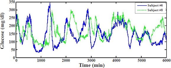
Subcutaneous glucose measurements for approximately 5 consecutive days with the iSense continuous glucose monitoring system for two typical individuals, subject #6 (continuous line) and subject #8 (dotted line), with type 1 diabetes.

To determine if AR models can represent glucose data by fully capturing the correlations in the time series, we first develop an AR model for a specific subject using a portion of time-series data of that subject and then, using the developed model, compute the prediction residuals of the series, i.e., the point-by-point difference between measured and predicted glucose values. The top panel in Figure 2 shows the measured and (1-minute ahead) predicted glucose levels obtained with an AR model of order m = 10 using the first 2000 minutes, i.e., the first 2000 data points, of subject's #6 data. The prediction residuals, illustrated in the bottom panel of Figure 2, are small, indicating a good model fit.

Figure 2.

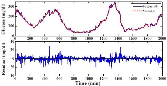
Model fit and residual error. Model fit for subject #6 based on an autoregressive model using the first 2000 minutes or data points (top) and corresponding residual error between model fit and sensor data (bottom).

Moreover, to determine the capability of the model fit in capturing correlations in time-series glucose data, we compute the autocorrelation of the residuals and check for whiteness in the correlation.¹² An appropriate model that fully captures the correlation in the data should result in uncorrelated residuals, consisting of white noise. For purely white noise residuals, the autocorrelation coefficients, normalized between −1 and 1, attain a value equal to one for a zero shift (i.e., zero delay) and a value equal to zero for all other shifts in the signal. For practical applications, where the residuals are not purely white and the autocorrelation coefficients for nonzero shifts hover around zero, a degree of certainty of the whiteness of the residuals may be inferred by computing approximate confidence intervals around the autocorrelation coefficients.

Figure 3 shows the autocorrelation function of the residual error corresponding to subject's #6 model depicted in Figure 2. The approximated 95% confidence intervals of the autocorrelation coefficients about zero, determined by the Portmanteau test,¹² are illustrated by the shaded area. Figure 2 suggests that the 10th-order AR model captures most of the correlations in glucose data, but not all of them. This is evidenced by the apparent structure remaining in the residuals, leading to minor but noticeable sinusoidal-type oscillations. This could be because of misspecification of the selected regression model. A model that completely captures the correlations in data for a specific subject, however, is not necessarily the best overall model if we wish the model to have good generalization capabilities and be portable from individual to individual.

Figure 3.

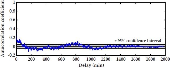
Autocorrelation function and associated 95% confidence interval of the model fit in Figure 2.

Next, we investigate the predictive power of AR models by determining the accuracy of the glucose-level predictions as a function of prediction horizon. Employing the AR model discussed earlier, developed by using the first 2000 minutes of subject's #6 data, we predict this subject's glucose levels for the remaining 4000 minutes for arbitrarily selected but clinically useful 30-, 60-, and 120-minute prediction horizons (Figure 4). That is, the prediction at any given time point in the future is performed 30, 60, or 120 minutes prior to that time. For example, predictions at 3000 minutes are performed at 2970, 2940, and 2880 minutes, respectively, for 30-, 60-, and 120-minute prediction horizons. As expected, the prediction accuracy decreases as the prediction horizon increases. This may be quantified by computing the root mean square error (RMSE) between measured and predicted glucose levels over the 4000 predicted points. Figure 4 shows that while predictions for the 30-minute horizon are quite accurate, exhibiting a small prediction delay and an RMSE of 22.2 mg/dl, the accuracy of the predictions deteriorates for longer horizons, indicating considerable phase shifts and a larger RMSE (53.8 mg/dl) for the 120-minute-ahead predictions.

Figure 4.

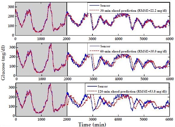
Autoregressive model predictions for subject #6 for three different prediction horizons: 30 minutes (top), 60 minutes (middle), and 120 minutes (bottom). The first 2000 minutes or data points (shaded area) are used to “learn” the model coefficients, and the predictions are performed over the remaining 4000 data points (6-6 results). The root mean square error (RMSE) is used as a metric to quantify the predictions between 2000 and 6000 minutes.

To further assess the utility of the predictions using clinically acceptable metrics, we perform Clarke error grid analysis,¹³ which maps pairs of sensor-predicted glucose concentrations into five zones, A to E, of varying degrees of accuracy and inaccuracy of glucose estimations. Values in zones A and B are clinically acceptable, whereas values in zones C, D, and E are potentially dangerous, with an increasing chance of incorrect treatment as the points move from zones C to D to E.

The Clarke error grid in Figure 5 shows the 30-minute prediction horizon results associated with the corresponding 4000 predictions in Figure 4. The results are also summarized in Table 1 (under the column marked 6-6, used to indicate that a model derived based on subject's #6 data is used to predict subject #6). The majority of the points (85.3%) lie in zone A, 13.3% in zone B, and the remaining 1.4% in zone D. Table 1 also shows results for the corresponding 60-minute prediction horizon, where 66.2% of the pairs lie in zone A, 31.1% in zone B, 0.6% in zone C, and 2.1% in zone D.

Figure 5.

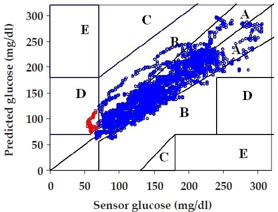
Clarke error grid analysis for 30-minute prediction horizon for the last 4000 data points of subject's #6 data using a model based on that subject's first 2000 data points (6-6 results in the top panel of Figure 4). Over 85% of the pairs fall in zone A, over 13% in zone B, and about 1% in zone D.

Table 1.

Clarke Error Grid Analysis for 30- and 60-minute Prediction Horizons for AR Models Based on Subjects #6 and #8^a Prediction horizon

	Prediction horizon
	30 min				60 min
	Model-Subject				Model-Subject
Zone	6-6	6-8	8-6	8-8	6-6	6-8	8-6	8-8
A	85.3%	84.4%	82.2%	90.0%	66.2%	64.2%	60.7%	72.9%
B	13.3%	14.2%	15.0%	9.8%	31.1%	32.5%	32.9%	25.1%
C	0.0%	0.0%	0.0%	0.0%	0.6%	0.2%	0.8%	0.0%
D	1.4%	1.4%	2.8%	0.2%	2.1%	3.1%	5.4%	2.0%
E	0.0%	0.0%	0.0%	0.0%	0.0%	0.0%	0.0%	0.0%

^aFor predictions based on models derived from the subject's own data (6-6 and 8-8), the analysis is performed on the last 4000 data points. For portable models, where a model based on subject's #6 data is used to predict subject #8 (6-8), as illustrated in Figure 6, and vice versa (8-6), as illustrated in Figure 7, the analysis is performed over the entire range of the predicted 6000 data points.

The Clarke error grid is used here (as one of two performance metrics) because of its clinical acceptability and as a common basis for comparison with other glucose-management algorithms.³ We note, however, that it has limitations in assessing the performance of CGM devices.¹⁴ In particular, it does not account for temporal dependencies in the signal and only provides a composite analysis, where all errors are treated equally (as a percentage) without accounting for consistent errors.

Finally, to determine the possibility of having AR models made portable from individual to individual without any need for model tuning, we apply the model developed using subject's #6 data to predict the entire glucose-level profile (6000 minutes) of subject #8 for the three prediction horizons (6-8 results in Figure 6). The results are very similar (in terms of RMSE) to those in Figure 4, where a model developed using subject's #6 data is used to predict unseen data for subject #6 (6-6), and to those obtained when the first 2000 minutes of subject's #8 data are used to predict that subject's remaining 4000 minutes (8-8 results not shown). The results are also similar in terms of the Clarke error grid analysis in Table 1. When comparing 8-8 results with 6-8 results, we notice that there is only a slight deterioration in the percentage of points falling in zones A plus B, for both 30- and 60-minute prediction horizons, when subject's #6 model is used to predict subject #8.

Figure 6.

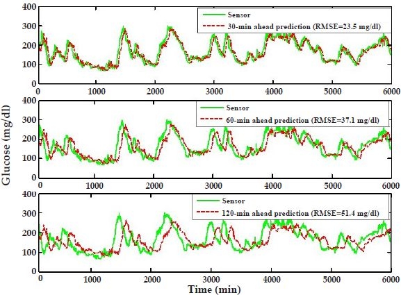
Autoregressive model predictions where the model based on the first 2000 minutes of subject's #6 data is employed to predict subject #8 (6-8 results). The predictions are provided for three prediction horizons: 30 minutes (top panel), 60 minutes (middle panel), and 120 minutes (bottom panel).

Similarly, Figure 7 shows the results when a model developed using the first 2000 minutes of subject's #8 data (with order m = 10) is used to predict the entire glucose-level profile for subject #6 (8-6 results). Comparison of the prediction accuracy over the last 4000 minutes between this model and the one developed using subject's #6 data indicates modest deterioration, with 8-6 results (Figure 7) showing slightly higher RMSEs than 6-6 results (Figure 4). The Clarke error grid analysis in Table 1 indicates that there is a small degradation when subject's #8 model is used to predict subject #6 (8-6 versus 6-6), suggesting that results achieved with portable models are not significantly inferior from those obtained with individually-tuned models.

Figure 7.

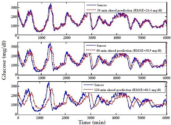
Autoregressive model predictions where the model based on the first 2000 minutes of subject's #8 data is employed to predict subject #6 (8-6 results). The predictions are provided for three prediction horizons: 30 minutes (top panel), 60 minutes (middle panel), and 120 minutes (bottom panel).

These results suggest that there is very small interindividual variability in the autocorrelation of time-series glucose data. Indeed, comparative analysis of the AR model coefficients b for subjects #6 and #8 indicates that the three most significant (latest) coefficients, which are orders of magnitude larger than the remaining seven coefficients, are very similar.

To provide further evidence of the portability of AR models, we perform cross-subject predictions over all nine subjects who passed the modeling exclusion criteria. Table 2 shows the comparison of two sets of predictions for each subject on the basis of RMSE and Clarke error grid analysis (zones A plus B). In the first set, predictions for each subject are obtained by using the subject's first 2000 minutes to develop the subject's model (with m = 10), which is subsequently used to predict the remaining 4000 minutes of glucose data (labeled as “self”). In the second set, each subject's model, developed as discussed earlier, is used to predict the entire glucose profile (6000 minutes) for each of the other eight subjects. The entries in Table 2 for these cross-subject predictions indicate average results and associated standard deviations for each subject based on predictions for that subject employing the models of the other eight subjects (“cross-subject”).

Table 2.

Comparison of Individually Tuned (Self) and Portable (Cross-Subject) Model Performance for the Nine Subjects Who Passed Modeling Exclusion Criteri^a Subject

Subject	Model	Prediction horizon
		30 min		60 min
		Root mean square error (mg/dl)	Clarke error grid % (A+B)	Root mean square error (mg/dl)	Clarke error grid % (A+B)
2	Self	17.5	100.0	24.8	99.8
	Cross-subject	21.1 ± 0.8	99.7 ± 0.0	30.4 ± 1.1	99.7 ± 0.0
6	Self	22.2	98.6	35.0	97.3
	Cross-subject	25.9 ± 1.3	95.8 ± 1.0	40.1 ± 1.0	90.9 ± 2.7
8	Self	20.9	99.8	33.6	98.0
	Cross-subject	24.8 ± 1.5	98.7 ± 0.4	37.9 ± 1.0	96.2 ± 0.4
9	Self	26.8	99.6	40.1	98.9
	Cross-subject	26.0 ± 1.3	99.6 ± 0.1	38.3 ± 0.7	99.0 ± 0.2
11	Self	29.6	99.0	41.1	98.4
	Cross-subject	30.8 ± 0.4	99.2 ± 0.1	41.5 ± 0.4	98.1 ± 0.3
12	Self	24.0	97.6	36.0	95.3
	Cross-subject	26.9 ± 1.3	97.8 ± 0.8	40.2 ± 1.0	95.2 ± 0.6
13	Self	20.0	99.3	29.5	98.6
	Cross-subject	24.6 ± 1.3	98.2 ± 0.2	36.1 ± 0.7	96.6 ± 0.1
14	Self	19.2	99.0	25.5	98.8
	Cross-subject	20.6 ± 1.1	98.6 ± 0.2	28.1 ± 0.5	97.6 ± 0.5
15	Self	20.1	98.7	25.7	97.4
	Cross-subject	22.3 ± 0.7	95.9 ± 1.4	29.4 ± 0.7	92.5 ± 2.4

^aFor results based on individually tuned models, analysis is performed on the last 4000 data points. For cross-subject models, where the results for each subject are averaged over the other eight model predictions using their own individualized models, analysis is performed for the entire range of the predicted 6000 data points. Their standard deviation over the other eight predictions is also illustrated.

Table 2 shows that, as expected, for both metrics the 30-minute-ahead predictions are consistently more accurate than the 60-minute predictions. In terms of Clarke error grid, for 30-minute-ahead predictions, 95.8 to 100.0% of the results fall in the clinically-acceptable zones A and B. More significantly, results indicate that there is only a modest decrement in performance between individually- tuned, self-models and cross-subject, portable models. For example, for the 30-minute-ahead predictions, the maximum decrement in performance, observed in both subjects #6 and #15, is of only 2.8 basis points (98.6– 95.8 for #6). Of additional importance is the negligible variance of the cross-subject results for each one of the nine subjects, indicating that the model of any one subject is capable of adequately predicting each of the other eight subjects. These results strongly support the hypothesis that AR models can be made portable.

Discussion

This study shows that data-driven autoregressive models, when regularized properly, provide very accurate and clinically acceptable, short-term predictions of glucose levels and should be considered as the forecasting engine for predictive monitoring of patients with type 1 diabetes mellitus. With sensor data serving as the gold standard, Clarke error grid analysis indicates that for 30-minute-ahead predictions, individually tuned models yield 97.6 to 100.0% of data in the clinically-acceptable zones A and B, whereas cross-subject, portable models yield 95.8 to 99.7% of the data in zones A and B (Table 2).

Data-driven AR models are particularly attractive because, due to the complexity of the underlying physiology of diabetes regulation coupled with the nonlinear dynamics of insulin action and glucose kinetics,³ accurate, individual-specific first-principal models capable of accounting for meals and physical activity are currently unavailable. As shown here, if provided with sufficient and representative data, AR models can generalize well across different portions of an individual's data and across individuals without jeopardizing their predictive capabilities.

A very recent parallel effort by the Cobelli group has also suggested the use of CGM and AR models for short-term glucose-level predictions of type 1 diabetes patients.¹⁵ Although they also found AR models to provide adequate results for 30-minute-ahead predictions, their modeling formulation is significantly different than ours. In particular, they found that models with an order larger than one and with fixed parameters to be unstable and yield unacceptable prediction delays. Accordingly, their AR model of order m = 1 is updated continuously (for each individual) as each new observation becomes available, and to avoid model “over fit” the parameter update balances the weight among current and prior observations. This is in sharp contrast with our approach, where an AR model is developed once for one individual and the same model is applied, without further model development or parameter adjustments, to predict other individuals. We hypothesize that this capability is because of the higher sampling rate of CGM data available to us (1 minute vs 3 minutes) and the use of regularization in computing the model parameters.¹¹

The power of AR models for short-term predictions stems from the long time delay or large time constant of the human-body glucose regulation process in response to insulin delivery or following a meal. For example, the onset of rapidly acting insulin occurs approximately within 10–15 minutes, peaking around 90 minutes. This long time delay between insulin delivery and its peak action results from the superposition of delays associated with insulin absorption from the subcutaneous depot and the duration of insulin action.³ Similarly, the onset of short-acting insulin occurs within 15–30 minutes, peaking around 150 minutes, while the onset of meal responses on glucose levels, generally larger than 5–10 minutes, can vary depending on food content.

It is this relatively large time constant of the glucose regulation process that allows AR models to employ previously learned correlations in glucose time-series data to predict future glucose levels accurately. The optimum, i.e., the longest useful prediction horizon, is therefore dependent on the time constant of glucose regulation, which may vary slightly dependent on the type of insulin and food content, and the desired prediction accuracy, with accuracy deteriorating with increasing horizons. A range of optimum prediction horizons could be established by considering the type of insulin/food that yields the shortest time constant and the lowest-acceptable prediction accuracy. This would require the design of a clinical study to collect necessary data. Nevertheless, preliminary results indicate that we can conservatively use AR models for short-term predictions of at least 30-minutes ahead to provide sufficiently accurate and clinically acceptable predictions for timely proactive therapy.

The data-driven AR models rely entirely on the correlations of glucose time-series data, which we find not to exhibit any considerable interindividual variability, provided individuals are involved in similar activities. An attractive implication of this result is that a data-driven model developed based on data from just one individual could be used to predict glucose levels for other individuals, yielding portable models and considerably reducing—if not completely eliminating—the burden associated with model tuning and data collection for model development. Further investigation is needed, however, to study other types of regression models, the effects of CGM sampling rate on model order, prediction delay and prediction horizon, and whether models can be made portable for subjects involved in strenuous physical activity, as the subjects used in this study were only allowed to perform mild physical activity in a structured and controlled environment.

The prediction of physiological variables should also be accompanied by a measure of reliability of the model predictions, for example, in the form of error bounds. In this respect, confidence and prediction intervals can be derived analytically for linear AR models¹⁶ or estimated through statistical bootstrap methods for nonlinear data-driven models.¹⁷

The coupling of continuous glucose monitoring devices with forecasting mathematical models could provide a distinct improvement to the glucose control continuum, yielding predictive monitoringof glucose levels, which would allow for proactive rather than reactive glucose regulatory interventions to adjust glucose levels before damage occurs. Predictive monitoring of glucose is within reach, as advances are made in CGM devices to improve biocompatibility and extend duration of use, and the mathematical modeling community makes contributions to this field to improve the fidelity of individual-specific forecasting models applicable across the entire spectrum of human activities.

Abbreviations

AR

autoregressive

BG

blood glucose

BMI

body mass index

CGM

continuous glucose monitoring

HbA1c

glycated hemoglobin

LS

least squares

SD

standard deviation

RMSE

root mean square error

References

- 1.Van den Berghe G. How does blood glucose control with insulin save lives in intensive care? J Clin Invest. 2004 Nov;114(9):1187–1195. doi: 10.1172/JCI23506. [DOI] [PMC free article] [PubMed] [Google Scholar]
- 2.Ludvigsson J, Hanas R. Continuous subcutaneous glucose monitoring improved metabolic control in pediatric patients with type 1 diabetes: a controlled crossover study. Pediatrics. 2003 May;111(5 Pt 1):933–938. doi: 10.1542/peds.111.5.933. [DOI] [PubMed] [Google Scholar]
- 3.Hovorka R, Canonico V, Chassin LJ, Haueter U, Massi-Benedetti M, Federici MO, Pieber TR, Schaller HC, Schaupp L, Vering T, Wilinska ME. Nonlinear model predictive control of glucose concentration in subjects with type 1 diabetes. Physiol Meas. 2004 Aug;25(4):905–920. doi: 10.1088/0967-3334/25/4/010. [DOI] [PubMed] [Google Scholar]
- 4.Bequette BW. A critical assessment of algorithms and challenges in the development of a closed-loop artificial pancreas. Diabetes Technol Ther. 2005 Feb;7(1):28–47. doi: 10.1089/dia.2005.7.28. [DOI] [PubMed] [Google Scholar]
- 5.Steil GM, Clark B, Kanderian S, Rebrin K. Modeling insulin action for development of a closed-loop artificial pancreas. Diabetes Technol Ther. 2005 Feb;7(1):94–108. doi: 10.1089/dia.2005.7.94. [DOI] [PubMed] [Google Scholar]
- 6.Gribok A, McKenna T, Reifman J. Regularization of body core temperature prediction during physical activity; Proceedings of the IEEE International Conference of Engineering in Medicine and Biology Society; New York City, New York. 2006. [DOI] [PubMed] [Google Scholar]
- 7.Box GEP, Jenkins GM, Reinsel GC. Time series analysis, forecasting and control. 3rd ed. Englewood Cliffs (NJ): Prentice Hall; 1994. [Google Scholar]
- 8.Ljung L. System identification: theory for the user. Englewood Cliffs (NJ): Prentice Hall; 1999. [Google Scholar]
- 9.Portland, Oregon: Sense Corporation; Available from: www.isensecorp.com (accessed on 3 January 2007) [Google Scholar]
- 10.Cherkassky V, Mulier F. Learning from data: concepts, theory and methods. Washington: Winston; 1998. [Google Scholar]
- 11.Tikhonov AN, Arsenin VY. Solutions of ill-posed problems. New York: Wiley; 1977. [Google Scholar]
- 12.Chatfield C. The analysis of time-series: an introduction. 6th ed. Boca Raton (FL): Chapman & Hall/CRC Press; 2004. [Google Scholar]
- 13.Clarke WL, Cox D, Gonder-Frederick LA, Carter W, Pohl SL. Evaluating clinical accuracy of systems for self-monitoring of blood glucose. Diabetes Care. 1987 Sep–Oct;10(5):622–628. doi: 10.2337/diacare.10.5.622. [DOI] [PubMed] [Google Scholar]
- 14.Kovatchev BP, Gonder-Frederick LA, Cox DJ, Clarke WL. Evaluating the accuracy of continuous glucose-monitoring sensors: continuous glucose-error grid analysis illustrated by TheraSense Freestyle Navigator data. Diabetes Care. 2004 Aug;27(8):1922–1928. doi: 10.2337/diacare.27.8.1922. [DOI] [PubMed] [Google Scholar]
- 15.Sparacino G, Zanderigo F, Corazza S, Maran A, Facchinetti A, Cobelli C. Glucose concentration can be predicted ahead in time from continuous glucose monitoring sensor time-series. IEEE Trans Biomed Eng. 2007 May;54(5):931–937. doi: 10.1109/TBME.2006.889774. [DOI] [PubMed] [Google Scholar]
- 16.Chatfield C. Time-series forecasting. Boca Raton (FL): Chapman & Hall/CRC Press; 2001. [Google Scholar]
- 17.Oleng' NO, Gribok A, Reifman J. Error bounds for data-driven models of dynamical systems. Comp Biol Med. 2007 May;37(5):670–679. doi: 10.1016/j.compbiomed.2006.06.005. [DOI] [PubMed] [Google Scholar]