Hypoglycemia Detection and Prediction Using Continuous Glucose Monitoring—A Study on Hypoglycemic Clamp Data

Abstract

Motivation

The fear of hypoglycemia remains an important limiting factor in the ability of an individual with type 1 diabetes to tightly regulate glycemia. Continuous glucose monitors provide important feedback to improve glycemic control, but there remains a need for these devices to better alarm of possible impending hypoglycemia, particularly overnight or other periods when the individual is engaged in activities that take their focus away from glucose monitoring.

Methods

We have previously proposed an algorithm, based on the use of real-time glucose sensor signals and optimal estimation theory (Kalman filtering), to predict hypoglycemia; the algorithm was validated in simulation-based studies. In this article we further refine and validate the prediction algorithm based on the analysis of clinical hypoglycemic clamp data from 13 subjects. The sensitivity and specificity of the predictions are calculated with respect to reference blood glucose values obtained at the same sampling rate of the sensor.

Results

For a 30-minute prediction horizon and alarm threshold of 70 mg/dl, the sensitivity and specificity were 90 and 79%, respectively, indicating that a 21% false alarm rate must be tolerated to predict 90% of the hypoglycemic events 30 minutes ahead of time. Shorter prediction horizons yield a significant improvement in sensitivity and specificity.

Discussion

Sensitivity and specificity data as a function of prediction horizon and alarm threshold enable an individual to adjust the alarm to best meet their needs. Such decisions can be made depending on the subject's risk for hypoglycemia, for example.

Motivation

People with type 1 diabetes have to balance their desire for maintaining tight glycemic control with the risk for iatrogenic hypoglycemia.¹ Even with recent advances in technology, hypoglycemia remains a limiting factor.

Bremer and Gough² first suggested that future glucose values might be predictable using continuous glucose monitoring (CGM) data, with the obvious application of anticipating hypoglycemia and other events. This sparked some further research efforts to accomplish this.^3–5 The most recent contribution in this area is that of Sparacino et al.,⁶ who use first-order polynomial and autoregressive models for which they estimate the model parameters using a recursive weighted least-squares framework.

We previously proposed an approach to predicting hypoglycemia in real-time using optimal estimation theory.⁷ In that study, the approach was demonstrated using simulated data, and we showed the trade-offs inherent among the sampling rate of the glucose sensor, the threshold selection, and, more importantly, the prediction horizon.

In this study we apply the same approach to retrospective clinical data and show the viability of the optimal estimation method.

Methods

There are two challenges when testing a real-time blood glucose prediction algorithm with clinical data. One is the necessity of having frequently sampled reference blood glucose values for comparison. The other is that there is a need to separate the performance of the sensor itself from that of the prediction algorithm.

We use data from a series of hypoglycemic clamps, in which a continuous glucose sensor (CGMS®, Medtronic MiniMed, Inc., Northridge, CA) is used. Reference blood glucose measurements are taken every 5 minutes for the duration of the procedure, providing the necessary data to evaluate the algorithm. The database used (courtesy of the University of Virginia General Clinical Research Center, with funding from the National Institutes of Health Grant R01-DK-51562) contains 76 distinct clamp procedures. Of these, only those that showed good performance of the sensor were selected for analysis, as otherwise it would be impossible to tell if the performance in prediction is due to the algorithm itself or to the calibration routine of the sensor. Selection criteria were median and mean relative absolute differences (RAD) less than 12% between the sensor and the reference blood glucose values. Only 13 of the clamp procedures met this requirement (median RAD 7.4 ± 1.6% and mean RAD 9.0 ± 1.7%).

The hypoglycemia prediction algorithm is described in detail in Palerm et al.⁷ For completeness, the algorithm is summarized here. Predictions are made using an estimate of the rate of change of the blood glucose, using a Kalman filter (an optimal estimation method). The Kalman filter trades off the probability that a measured glucose change is due to sensor noise versus an actual change in glucose, to obtain the maximum likelihood estimate of glucose (and its first and second derivatives). In this case, the model is given by

$$\underset{x_{k+1}}{\underbrace{\left[\begin{array}{c}{g}_{k+1}\\ d_{k+1}\\ f_{k+1}\end{array}\right]}}=\underset{\Phi }{\underbrace{\left[\begin{array}{ccc}1& 1& 0\\ 0& 1& 1\\ 0& 0& 1\end{array}\right]}}\underset{x_k}{\underbrace{\left[\begin{array}{c}{g}_k\\ d_k\\ f_k\end{array}\right]}}+\underset{{\Gamma }^W}{\underbrace{\left[\begin{array}{c}0\\ 0\\ 1\end{array}\right]}}{w}_k$$ (1a)

$$y_k=\underset{C}{\underbrace{\left[\begin{array}{ccc}1& 0& 0\end{array}\right]}}\left[\begin{array}{c}{g}_k\\ d_k\\ f_k\end{array}\right]+{\upsilon }_k$$ (1b)

where the indices k and k + 1 denote the current time step and one time step into the future, respectively. The states are the blood glucose concentration (g_k), its rate of change (d_k, i.e., the velocity), and the rate of change of the rate of change (f_k, i.e., the acceleration). The latter is assumed to vary in a random fashion, driven by the input noise w_k (with covariance matrix Q), which describes changes to the process. The blood glucose measurements are assumed to contain noise, described by υ_k (with covariance matrix R).

The Kalman filter uses a two-step process. It first calculates the estimate of the states (denoted by ◯) using the model based on the information up to the previous time step. Then

$${\widehat{x}}_{k|k-1}=\Phi {\widehat{x}}_{k-1|k-1}$$ (2)

where the subscript k|k − 1 indicates the estimate at time step k, using measurements up to time step k − 1.

Once the measurement at time step k is available, it is used to correct the estimate of the states, using

$${\widehat{x}}_{k|k}={\widehat{x}}_{k|k-1}+L(y_k-C{\widehat{x}}_{k|k-1})$$ (3)

where L is the steady-state Kalman gain and ($C{\widehat{x}}_{k|k-1}$) is the difference between the measured output and the expected output using the estimate from Equation (2). The Kalman gain L is calculated using the covariances Q and R. Given that these covariances are not known in advance, they become tuning parameters. Changing the relative weight between Q and R serves to trade off the confidence in the model versus the confidence in the measurement. Putting a significant weight on the trust in the measurement means that the estimates will track the sensor signal very closely, even if noisy. Conversely, weighing the model significantly more than the measurement results in a heavily filtered estimate. The tuning is thus selected manually based on the best trade-off sought between these two extremes, which in this case is done as to maximize the sensitivity and specificity of the hypoglycemia predictions. For example, when Q/R = 1.25e-3 then L = [0.4821 0.1699 0.0254]^T.

The model [Equation (1)] can then be used to estimate blood glucose into the future. Prediction horizons from 5 to 30 minutes are considered (in 5-minute increments). The algorithm is tuned to maximize the sensitivity and specificity over all of the data sets. This is done for each of the prediction horizons independently. As in the initial study, hypoglycemia is defined to be blood glucose below 70 mg/dl. Different thresholds for predicting hypoglycemia are considered, from 60 to 90 mg/dl (in 5-mg/dl increments), but always setting true hypoglycemia to be below 70 mg/dl.

The prediction algorithm estimates, in real time, the first and second derivatives of blood glucose. When making predictions, particularly at longer prediction horizons, the assumption that the second derivative remains constant at a nonzero value might not hold. For this reason the results are compared when the second derivative is used in making the actual predictions ($f_{k+i|k}=f_{k|k}\mathbf{\forall }i\in$ prediction horizon) versus the case when it is considered to be zero ($f_{k+i|k}=0\mathbf{\forall }i\in$ prediction horizon).

Results

Hypoglycemic clamp procedures start with elevated blood glucose, and glucose levels are brought close to 100 mg/dl before inducing hypoglycemia. During the initial phase of the clamp, blood glucose drops at a rate of 1.3 ± 0.6 (1.2 [0.6–2.7]) mg/dl mean ± standard deviation (median [range]). In the period when hypoglycemia is induced, the rate of change is significantly lower, at 0.9 ± 0.1 (0.9 [0.8–1.2]) mg/dl. This poses a challenge to the prediction algorithm, as the rate of change of blood glucose is manipulated during the clamp with intravenous infusions of insulin and glucose, with the more aggressive changes taking place in the initial phase. Such fast changes will invariably lead to false positives over longer prediction horizons.

The tuning of the estimation algorithm in relation to the prediction horizon had not been explored previously. In Palerm et al.,⁷ the same tuning was used for all prediction horizons. Tuning the algorithm to maximize the sensitivity and specificity over the different prediction horizons resulted in different optimal settings. The setting that provided the best performance for the longer prediction horizon (30 minutes, Q/R = 0.04) was 30 times larger than the one for the shortest prediction horizon (5 minutes, Q/R = 0.0013). For the remainder of the data analysis the best tuning for each prediction horizon is used.

Figure 1 shows a comparison of the sensor and reference blood glucose, together with the predictions made 10, 20, and 30 minutes into the future. Figure 1A shows the case when the second derivative is not used to make predictions, and Figure 1B shows when it is used. These results show that for the shorter prediction horizon (10 minutes), the results are almost identical, but as the prediction horizon is extended, the decrease in performance when using the second derivative for making the predictions becomes significant.

Figure 1.

Comparison of the predictions for horizons of 10, 20, and 30 minutes into the future for one of the clamp procedures. In both cases it is clear how longer prediction horizons degrade performance. Setting the second derivative to zero (A) improves blood glucose predictions as compared to the case when it is used (B).

Over all the data sets, the sensitivity and specificity of the predictions were calculated for the different prediction horizons and detection thresholds. Given that reference blood glucose measurements are provided at the same sampling frequency as the continuous glucose sensor signal, a point-by-point comparison is done to calculate sensitivity and specificity. Therefore, for a prediction made at time k for time k + 3, the corresponding reference blood glucose value at time k + 3 used to determine if the prediction of hypoglycemia/no hypoglycemia was a true or false positive/negative. Figure 2 clearly shows the trade-off between sensitivity and specificity for different choices of prediction horizon and detection threshold. Use of the second derivative in making the predictions, Figure 2B, also shows decreased performance over the longer prediction horizons, with slightly lower sensitivity and specificity, and greater variability.

Figure 2.

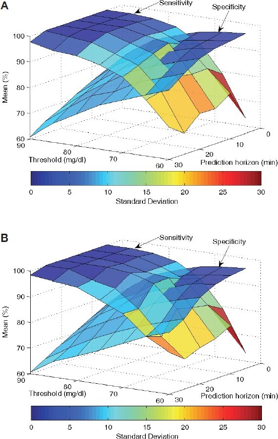
Sensitivity and specificity depend on the prediction horizon, as well as the threshold used to decide on hypoglycemia. Setting the second derivative to zero (A) also improves the sensitivity and specificity of the blood glucose predictions as compared to the case when it is used (B).

Figure 3 shows the receiver operating characteristic (ROC) curve for three different prediction horizons. The threshold in all cases with the lowest sensitivity corresponds to a threshold of 60 mg/dl. As the threshold is increased (in increments of 5 mg/dl) up to 90 mg/dl, the sensitivity improves, at the expense of the specificity. As with Figure 2, it is clear that the longer the prediction horizon is, the worse the performance is overall.

Figure 3.

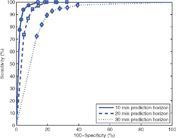
ROC curves for prediction horizons of 10, 20, and 30 minutes. Marked points with the lowest sensitivity for each curve correspond to a threshold of 60 mg/dl. As the threshold is increased (markers are at 5-mg/dl intervals), the sensitivity improves, at the expense of specificity.

As expected, the choice of a higher detection threshold for hypoglycemia improves on the sensitivity of the algorithm, drastically reducing the number of missed true hypoglycemic events (those below 70 mg/dl). This comes at the expense of reduced specificity, significantly increasing the number of false positives. For use in a hypoglycemia alarm, there are then two settings that must be specified: the prediction horizon and the threshold. The prediction horizon will depend on how much warning is desired before going below 70 mg/dl, and the threshold will depend on how many false positives can be tolerated. In both cases, there is no correct answer and will depend greatly on user preference.

Discussion

The issue of reduced specificity is of concern, as it can lead to too frequent alarms that require no response from the subject. In this case, there will be an inclination to ignore the alarms and therefore miss the opportunity to take corrective action when the alarm is indeed warranted. Kovatchev and colleagues⁸ have shown that there is a measurable disturbance in blood glucose in a 48-hour period preceding severe hypoglycemic events. Using data from self-monitoring of blood glucose taken three to five times per day, they found a reduction in the blood glucose average and an increase in its variance. In particular, an increase in the low blood glucose index (LBGI)—a risk measure proposed by Kovatchev and co-workers⁹—correlated well with this increased risk of severe hypoglycemia.

We propose that such metrics can be used in the context of CGM to adjust the prediction horizon and threshold automatically depending on the risk for hypoglycemia. Cutoff values for the LBGI were proposed by Kovatchev et al.¹⁰ for low (LBGI < 2.5), moderate (2.5 ≤ LBGI ≤ 5), and high (LBGI > 5) risk for severe hypoglycemia. The LBGI average over the preceding 24-hour window can then be used to select the prediction horizon and threshold accordingly. In the case of low risk the objective would be to minimize false alarms, thus a shorter prediction horizon (e.g., 10 minutes) combined with a tight threshold (e.g., 75 mg/dl) could be used. As risk increases, the prediction horizon and/or the threshold can be increased, with the idea being that the subject will tolerate more false alarms when in high risk, but not when the risk is low. Computation of the LBGI using CGM can be done as described elsewhere.¹¹

We have shown that an algorithm based on optimal estimation theory is effective in making predictions of hypoglycemia. The choice of detection threshold and prediction horizon affects the sensitivity and specificity of the system. As with any such system, the selection of these parameters depends on the application, as well as on user preference.

Although these initial results applying the optimal estimation-based algorithm are very encouraging, there are other aspects that need to be studied. The previous study⁷ showed that more frequent sampling can significantly improve the sensitivity and specificity of the system for the same detection threshold and prediction horizon. Therefore, appropriate data using a continuous glucose sensor capable of providing more frequent glucose output (with a 1-minute sample time, for example) should be studied.

Abbreviations

CGM

continuous glucose monitoring

LBGI

low blood glucose index

RAD

relative absolute differences

ROC

receiver operating characteristic

References

- 1.Cryer PE. Hypoglycaemia: the limiting factor in the glycaemic management of type I and type II diabetes. Diabetologia. 2002 Jul;45(7):937–948. doi: 10.1007/s00125-002-0822-9. [DOI] [PubMed] [Google Scholar]
- 2.Bremer T, Gough DA. Is blood glucose predictable from previous values? A solicitation for data. Diabetes. 1999 Mar;48(3):445–451. doi: 10.2337/diabetes.48.3.445. [DOI] [PubMed] [Google Scholar]
- 3.Choleau C, Dokladal P, Klein J, Ward WK, Wilson GS, Reach G. Prevention of hypoglycemia using risk assessment with a continuous glucose monitoring system. Diabetes. 2002 Nov;51(11):3263–3273. doi: 10.2337/diabetes.51.11.3263. [DOI] [PubMed] [Google Scholar]
- 4.Heise T, Koschinsky T, Heinemann L, Lodwig V. Glucose monitoring Study Group. Hypoglycemia warning signal and glucose sensors: requirements and concepts. Diabetes Technol Ther. 2003;5(4):563–571. doi: 10.1089/152091503322250587. [DOI] [PubMed] [Google Scholar]
- 5.Ward WK. The role of new technology in the early detection of hypoglycemia. Diabetes Technol Ther. 2004 Apr;6(2):115–117. doi: 10.1089/152091504773731294. [DOI] [PubMed] [Google Scholar]
- 6.Sparacino G, Zanderigo F, Corazza S, Maran A, Facchinetti A, Cobelli C. Glucose concentration can be predicted ahead in time from continuous glucose monitoring sensor time-series. IEEE Trans Biomed Eng. 2007 May;54(5):931–937. doi: 10.1109/TBME.2006.889774. [DOI] [PubMed] [Google Scholar]
- 7.Palerm CC, Willis JP, Desemone J, Bequette BW. Hypoglycemia prediction and detection using optimal estimation. Diabetes Technol Ther. 2005 Feb;7(1):3–14. doi: 10.1089/dia.2005.7.3. [DOI] [PubMed] [Google Scholar]
- 8.Kovatchev BP, Cox DJ, Farhy LS, Straume M, Gonder-Frederick L, Clarke WL. Episodes of severe hypoglycemia in type 1 diabetes are preceded and followed within 48 hours by measurable disturbances in blood glucose. J Clin Endocrinol Metab. 2000 Nov;85(11):4287–4292. doi: 10.1210/jcem.85.11.6999. [DOI] [PubMed] [Google Scholar]
- 9.Kovatchev BP, Cox DJ, Gonder-Frederick LA, Clarke W. Symmetrization of the blood glucose measurement scale and its applications. Diabetes Care. 1997 Nov;20(11):1655–1658. doi: 10.2337/diacare.20.11.1655. [DOI] [PubMed] [Google Scholar]
- 10.Kovatchev BP, Cox DJ, Gonder-Frederick LA, Young-Hyman D, Schlundt D, Clarke W. Assessment of risk for severe hypoglycemia among adults with IDDM: validation of the low blood glucose index. Diabetes Care. 1998 Nov;21(11):1870–1875. doi: 10.2337/diacare.21.11.1870. [DOI] [PubMed] [Google Scholar]
- 11.Kovatchev BP, Clarke WL, Breton M, Brayman K, McCall A. Quantifying temporal glucose variability in diabetes via continuous glucose monitoring: mathematical methods and clinical application. Diabetes Technol Ther. 2005 Dec;7(6):849–862. doi: 10.1089/dia.2005.7.849. [DOI] [PubMed] [Google Scholar]