Accuracy Requirements for a Hypoglycemia Detector: An Analytical Model to Evaluate the Effects of Bias, Precision, and Rate of Glucose Change

Abstract

Background

There has been considerable debate on what constitutes a good hypoglycemia (Hypo) detector and what is the accuracy required from the continuous monitoring sensor to meet the requirements of such a detector. The performance of most continuous monitoring sensors today is characterized by the mean absolute relative difference (MARD), whereas Hypo detectors are characterized by the number of false positive and false negative alarms, which are more relevant to the performance of a Hypo detector. This article shows that the overall accuracy of the system and not just the sensor plays a key role.

Methods

A mathematical model has been developed to investigate the relationship between the accuracy of the continuous monitoring system as described by the MARD, and the number of false negatives and false positives as a function of blood glucose rate change is established. A simulation method with N = 10,000 patients is used in developing the model and generating the results.

Results

Based on simulation for different scenarios for rate of change (0.5, 1.0, and 5.0 mg/dl per minute), sampling rate (from 1, 2.5, 5, and 10 minutes), and MARD (5, 7.5, 10, 12.5, and 15%), the false positive and false negative ratios are computed. The following key results are from these computations.

1. For a given glucose rate of change, there is an optimum sampling time.

2. The optimum sampling time as defined in the critical sampling rate section gives the best combination of low false positives and low false negatives.

3. There is a strong correlation between MARD and false positives and false negatives.

4. For false positives of <10% and false negatives of <5%, a MARD of <7.5% is needed.

Conclusions

Based on the model, assumptions in the model, and the simulation on N = 10,000 patients for different scenarios for rate of glucose change, sampling rate, and MARD, it is concluded that the false negative and false positive ratio will vary depending on the alarm Hypo threshold set by the patient and the MARD value. Also, to achieve a false negative ratio <5% and a false positive ratio <10% would require continuous glucose monitoring to have an MARD ≤7.5%.

Introduction

There has been considerable debate on what constitutes a good hypoglycemia (Hypo) detector and what is the accuracy required from the continuous monitoring sensor to meet the requirements of such a detector.^1–9 This article shows that the overall accuracy of the system and not just the sensor plays a key role. Other errors introduced because of calibration, lag, drift, and so on play as big a role as sensor accuracy, if not more.

The performance of most continuous monitoring sensors today is characterized by the mean absolute relative difference (MARD), whereas Hypo detectors are characterized by the number of false positive and false negative alarms, which are more relevant to the performance of a Hypo detector.^1,3,4,6 A large number of false negative alarms can be life-threatening for the patient, whereas false positive alarms can be a nuisance to the point that the patient will not trust or use the device and may lead to the administration of unnecessary glucose, causing a disruption of glycemic control. Minimizing the number of false negative alarms and false positive alarms is a must. A good Hypo detector is expected to have false negative alarms and false positive alarms of less than 5 and 10%, respectively.

Problem Description

The true glucose level for a person at the starting point t₁ is G(t₁). A glucose monitoring system makes noisy glucose measurements $\widehat{\text{G}}\left({\text{t}}_{\text{n}}\right)$ for this person at prescribed time intervals t_n, with the degree of noisiness defined by both systemic bias and random variation. These actual blood glucose measurements are then used to detect a Hypo event below a predefined threshold level and to predict the true rate of decrease with respect to time by fitting a straight line to data and estimating the slope for the line. It is required to estimate the number of false positive alarms and false negative alarms based on the glucose measurement system.

Assumptions:

• Glucose levels at or below 70 mg/dl are considered hypoglycemic.

• Glucose levels below 55 mg/dl are considered critical.

• The true glucose change with respect to time is linear with slope bgr.

• There is a systematic bias in the actual blood glucose measurement of %b relative to the true glucose value. [A continuous glucose monitoring sensor is usually calibrated by the patient by entering a reference value obtained from a finger stick measurement using a commercially available device. The accuracy of commercially available devices is normally ±20% for glucose values above 100 mg/dl. The imprecision of this commercially available device contributes to the systematic bias. Other contributions to the systematic bias can include difference between interstitial fluid (ISF) and blood during probe calibration and drift of probe over time.]

• The imprecision of the actual glucose measurement follows a normal distribution with a CV of %cv relative to the true glucose value.

Sensor Accuracy

From the assumptions just listed, one can write

$$\widehat{\text{G}}\left({\text{t}}_{\text{n}}\right)=\text{G}\left({\text{t}}_{\text{n}}\right)+\%\text{b}\times \text{G}\left({\text{t}}_{\text{n}}\right)+\%\text{cv}\times \text{G}\left({\text{t}}_{\text{n}}\right)\times {\epsilon }_{\text{n}}$$ (1)

where G(t_n) is the true glucose level, $\widehat{\text{G}}\left({\text{t}}_{\text{n}}\right)$ is the noisy glucose measurement, %b is the systematic bias relative to the true glucose level, %cv is the coefficient of variation (%cv) due to the noise of the glucose measurement, and ε_n are independent standard normal random variables.

From Equation (1), the accuracy of a glucose measurement is plotted for different values of %b and %cv as illustrated in Figure 1.

Figure 1.

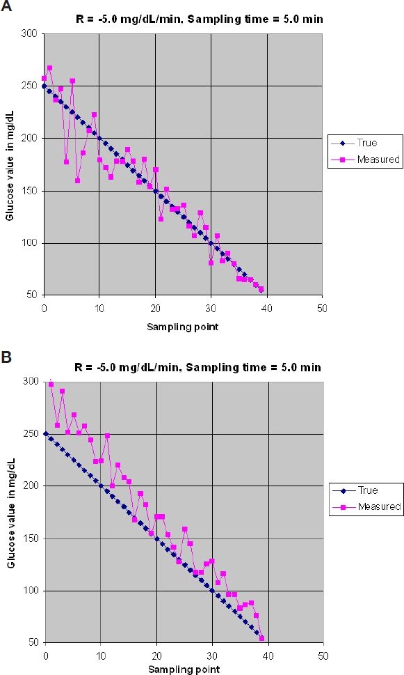
Accuracy of glucose measurement. (A) %b = 0%, %cv = 10%. (B) %b = 15%, %cv = 10%.

In Figure 1 it is assumed that the blood glucose rate is changing at −5.0 mg/dl/min and that the sampling rate is equal to a sample/5.0 min. In Figure 1A, the sensor has no bias (%b = 0%) and has a %cv of 10%. It can be noted that the glucose measurement is distributed randomly around the true value (blue line). In Figure 1B, the sensor has a bias %b = 15% and the precision is the same as in Figure 1A (%cv = 10%). In Figure 1B, a noticeable shift upward for the glucose measurement is introduced. The difference between results in Figure 1A vs Figure 1B is that an average of samples can improve the final results, while irrespective of the number of samples in Figure 1B, the average of the measured results will not get rid of the bias error.

Error in Calculating Rate of Change

This section derives a relationship between the accuracy of the blood glucose sensor measurement and the rate of change calculation. The rate of change of blood glucose is defined as (Figure 2)

$$\text{bgr}=\frac{\text{G}\left({\text{t}}_2\right)-\text{G}\left({\text{t}}_1\right)}{{\text{t}}_2-{\text{t}}_1}=\frac{\text{G}\left({\text{t}}_2\right)-\text{G}\left({\text{t}}_1\right)}{\Delta \text{t}}$$ (2)

Let us assume that the noisy blood glucose measurement at time t_n is given by Equation (1). The rate of change of blood glucose, $\text{bg}\widehat{\text{r}}$, estimated by performing a linear regression on noisy data

$$\left({\text{t}}_1,\widehat{\text{G}}\left({\text{t}}_1\right)\right),\cdots ,\left({\text{t}}_{\text{n}},\widehat{\text{G}}\left({\text{t}}_{\text{n}}\right)\right)$$

can be written as (see Section A.1 in the Appendix)

$$\text{bg}\widehat{\text{r}}=\text{bgr}+\text{b}\%\times \text{bgr}+\%\text{cv}\times \text{E}$$ (3)

where E is a normally distributed error with mean 0 and variance depending on (t₁, G(t₁)),…, (t_n, G(t_n)).

Figure 2.

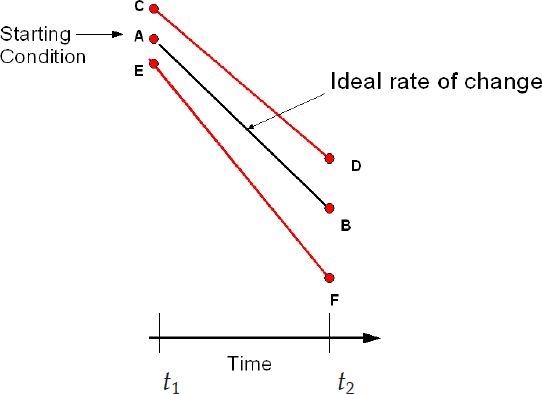
Rate of change.

Equation (3) shows that there is a systematic relative bias in the estimated blood glucose rate equal to the systematic relative bias in the blood glucose measurement.

Line AB in Figure 3 represents the ideal condition where A is the initial true glucose value at time t₁ = 0 and the glucose value is changing along AB at the true rate of change bgr. Based on the initial value of A and the rate of change bgr, the line AB will intersect the Hypo threshold level at a time t_Hypo given by Equation (4):

$$t_{Hypo}=\frac{\text{Hypo\hspace{0.17em}Threshold}-G\left(t_1\right)}{bgr}$$ (4)

Equations (1) and (3) show that start-up conditions for a nonideal sensor will differ from A (points C or E) and the rate of changes will be different along lines CD or EF. The actual Hypo time can be written as

$${\widehat{t}}_{Hypo}=\frac{\text{Hypo\hspace{0.17em}Threshold}-\widehat{G}\left(t_1\right)}{bg\widehat{r}}$$ (5)

Figure 3.

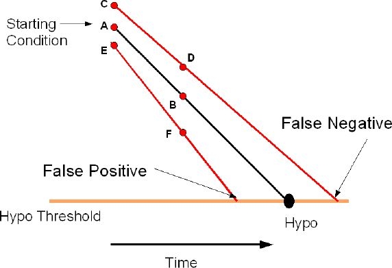
Effect of accuracy on Hypo detection.

If the actual time to intersection ${\widehat{\text{t}}}_{\text{hypo}}$ is less than t_hypo, then it is considered a false positive alarm. Conversely, if the actual time to intersection ${\widehat{\text{t}}}_{\text{hypo}}$ is greater than t_hypo, then it is considered a false negative alarm. Figure 3 shows that the percentage of false positive alarms and false negative alarms will vary depending on the values of the systematic bias %b and the coefficient of variation %cv. For a sensor with %b = 0%, the percentage of false positive alarms will be 50% and the percentage of false negative alarms will be 50% at time t = t_hypo. A positive bias will increase the percentage of false negative alarms while decreasing the percentage of false positive alarms, whereas a negative bias will decrease the percentage of false negative alarms while increasing the percentage of false positive alarms.

Alarm Threshold

If the Hypo threshold is defined as the level of glucose below which a patient is considered in a true Hypo state and an alarm or warning signal should be given and the critical Hypo threshold is the level we do not want any patient to reach or go below it, then a window in which alarms can be given can be described as shown in Figure 4.

Figure 4.

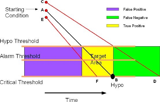
Effect of accuracy on Hypo detection.

Define

$${\text{t}}_{\text{upper}}=\frac{\text{Critical\hspace{0.17em}Threshold}-\text{G}\left({\text{t}}_1\right)}{\text{bgr}}$$ (6A)

$${\text{t}}_{\text{lower}}=\frac{\text{Hypo\hspace{0.17em}Threshold}-\text{G}\left({\text{t}}_1\right)}{\text{bgr}}$$ (6B)

An alarm prior to t_lower is a false positive alarm, whereas not providing an alarm after t_upper is a false negative alarm.

The box bounded by t_upper, t_lower, Hypo threshold, and critical threshold is the region of true positive alarms and is defined as the “target area.”

Intersections of the actual slope (line CD or line EF) with the alarm threshold result in an intersection time called t_actual:

$${\text{t}}_{\text{acutal}}=\frac{\text{Alarm\hspace{0.17em}Threshold}-\widehat{G}\left(t_1\right)}{\text{bg}\widehat{\text{r}}}$$ (7)

where t_actualgreater than t_upper is considered a false negative alarm, whereas a value of t_actual less than t_lower is considered a false positive alarm, respectively. By selecting the alarm threshold, the values of false positive alarms (false negative alarms) will vary from 0 to 100% depending on the values of the systematic bias %b and coefficient of variation %cv. As a result, it is possible for the patient to control the percentage of either false positive alarms or false negative alarms by selecting an appropriate alarm threshold.

False Positive and False Negative Ratio

In published papers, performance criteria of a continuous glucose monitoring sensor are described by the receiver operating characteristic chart and in terms of both sensitivity and specificity. Such an approach is based on measured values that are above or below a given threshold when compared to a reference value and does not take into account the time at which the event occurs. In this analysis, if an alarm occurs before or after the target area it is considered a false positive or false negative, respectively. In addition, it is assumed that the prevalence is 100%; in other words, we are focusing only on patients with Hypo events, which are different than sensitivity and specificity criteria, where prevalence is a small percentage of the overall patient population.

False positive and false negative ratios are defined as the ratio of the number of patients who get an alarm outside the “target area” (Figure 4) to the total number of patients with a Hypo event.

$$\text{False Positive\hspace{0.17em}}\%=\frac{\text{Number\hspace{0.17em}of\hspace{0.17em}patients\hspace{0.17em}who\hspace{0.17em}alarm\hspace{0.17em}before\hspace{0.17em}"Target\hspace{0.17em}Area"}}{\text{Total\hspace{0.17em}number\hspace{0.17em}of\hspace{0.17em}patients\hspace{0.17em}with\hspace{0.17em}Hypo\hspace{0.17em}event}}$$

$$\text{False Negative\hspace{0.17em}}\%=\frac{\text{Number\hspace{0.17em}of\hspace{0.17em}patients\hspace{0.17em}who\hspace{0.17em}alarm\hspace{0.17em}before\hspace{0.17em}"Target\hspace{0.17em}Area"}}{\text{Total\hspace{0.17em}number\hspace{0.17em}of\hspace{0.17em}patients\hspace{0.17em}with\hspace{0.17em}Hypo\hspace{0.17em}event}}$$

Critical Sampling Rate

From basic sampling theory (Nyquist–Shannon sampling theorem), it is known that in order to capture enough of a signal to be able to reconstruct it from discrete measurements, the sampling frequency must be at least twice that of the highest frequency contained in the signal. For patients with diabetes, it is harder to define such frequency because the mean glucose value, the peak and low excursions around the mean, and the maximum rate of change will vary from patient to patient. This article takes a different approach in defining the critical sampling rate. Figure 4 shows that if we want to guarantee three samples (three swings) within the “target area” (“baseball plate”), the sampling period can be selected in a fashion that allows for three samples to fall between t_upper and t_lower. From Equations (6A) and (6B), can be defined as

$${\text{t}}_{\text{critical}}=\left({\text{t}}_{\text{upper}}-{\text{t}}_{\text{lower}}\right)/3$$

and the critical sampling rate will be equal to

$$\text{Sampling\hspace{0.17em}}{\text{rate}}_{\text{critical}}\ge \frac{\text{1}}{{\text{t}}_{\text{critical}}}$$

where t_critical depends on the blood glucose rate of change, the Hypo threshold, and the critical threshold.

As shown in the simulation section, false positives and false negatives depend not only on the sampling rate, but also on the relative position of the samples with respect to t_upper and t_lower. In other words, when the samples fall exactly on t_upper and t_lower the false positive and false negative rates improve. In real life, we cannot guarantee that the samples will always coincide with t_upper and t_lower and in actuality the samples will be distributed randomly around t_upper and t_lower within ± Sampling rate_critical /2 impacting the false positive and false negative rates negatively.

Mean Average Relative Difference (MARD)

For a given patient making N measurements, the MARD is defined as

$$\text{MARD}=\frac{1}{\text{N}}\times {\displaystyle {\sum }_{\text{i}-1}^{\text{N}}\frac{\left|\widehat{\text{G}}\left({\text{t}}_{\text{i}}\right)-\text{G}\left({\text{t}}_{\text{i}}\right)\right|}{\text{G}\left({\text{t}}_{\text{i}}\right)}}$$ (8)

where N is the number of samples. Section A.2 in the Appendix derives an approximation to the MARD under the assumptions given later. This expression simplifies under the following conditions:

1. No imprecision (%cv = 0)

$$\text{MARD}=\left|\%\text{b}\right|$$ (9)

2. No bias and nonnegative imprecision (%b = 0, %cv > 0).

$$\text{MARD}\approx \text{0}\text{.80}\times \%\text{cv}$$ (10)

3. Bias large in absolute value relative to the imprecision (|%b| >> %cv)

$$\text{MARD}\approx \left|\%\text{b}\right|$$ (11)

Equations (9)–(11) show that there is a direct correlation between the MARD and the sensor accuracy. For a systematic relative bias of zero, MARD is proportional to the coefficient of variation, and when the systematic bias is large relative to the coefficient of variation, the MARD is equal to the absolute value of the bias.

Blood Glucose Rate of Change Estimate

Let us assume that the noisy blood glucose measurement at time t_n is given by Equation (1). We assume that the time step between consecutive samples is a constant for a given sampling rate and is equal to Δt. The rate of change of blood glucose, $\text{bg}\widehat{\text{r}}$, estimated by performing a linear regression on noisy data

$$\left({\text{t}}_1,\widehat{\text{G}}\left({\text{t}}_1\right)\right),\cdots \left({\text{t}}_{\text{n}},\widehat{\text{G}}\left({\text{t}}_{\text{n}}\right)\right)$$

can be written as (see Section A.1 in the Appendix)

$$\text{bg}\widehat{\text{r}}=\text{bgr}+\text{b}\%\times \text{bgr}+\%\text{cv}\times \text{E,}$$ (12)

where E is a normal random variable with mean 0 and variance

$$\frac{3}{{\text{N}}^3-\text{N}}\times \left\{\frac{\left(3\times {\text{N}}^2-7\right)}{5}\times {\left(\text{bgr}\right)}^2{\left(\frac{\text{G}\left({\text{t}}_1\right)+\text{G}\left({\text{t}}_{\text{n}}\right)}{\Delta \text{t}}\right)}^2\right\}.$$ (13)

Equation (13) shows that the variance of the slope estimate consists of two components. The first component depends on the true rate of change and is of order

$$\text{O}\left(\frac{1}{\text{N}}\right).$$

The second component depends on the average of the true glucose response and the sampling rate and is of order

$$\text{O}\left(\frac{1}{{\text{N}}^{\text{3}}}\right).$$

For a blood glucose measurement with high precision (%cv ≈ 0), Equation (12) is approximately equal to

$$\text{bg}\widehat{\text{r}}=\text{bgr}+\text{b}\%\times \text{bgr},$$ (14)

where the relative error in the glucose rate estimate is equal to the relative error in glucose measurement.

From Equations (13) and (14) two observations can be made:

1. The error because of bias cannot be improved by increasing the number of observations used in the regression

2. The error term decreases as the number of observations increases. Ultimately the error term decreases to zero as N→∞.

The number of points that can be used in the average will be dictated by the sampling rate, the initial glucose value, the rate of change, and the final value. For example, if the initial glucose value is 250 mg/dl, the sampling rate is 3 minutes, and the rate of change is −5.0 mg/dl/min, the maximum number of samples available before reaching the Hypo threshold of 70 mg/dl is

$$\text{N}=\frac{\left(70-250\right)/-5.0}{3}=12.$$

Based on Equation (13) the question becomes: Is it better to have fewer samples with a better precision or a large number of samples with less precision? Fix the number of observations, N, and the coefficient of variation, %cv, and let the sampling rate, Δt, vary. Only the last term on the right-hand side of Equation (13) is affected. That term can be rewritten as

$$\begin{array}{l}{\left(\frac{\text{G}\left({\text{t}}_1\right)+\text{G}\left({\text{t}}_{\text{n}}\right)}{\Delta \text{t}}\right)}^2={\left(\frac{\text{G}\left({\text{t}}_1\right)+\left(\text{G}\left({\text{t}}_1\right)+\text{N}\times \Delta \text{t}\right)}{\Delta \text{t}}\right)}^2\hfill \\ ={\left(\frac{2\times \text{G}\left({\text{t}}_1\right)}{\Delta \text{t}}+\text{N}\right)}^2\hfill \end{array}$$ (15)

From Equations (13) and (15) we can conclude

1. For a given coefficient of variation, %cv, a sensor with a faster sampling rate will require more samples to achieve the same error in the glucose rate calculation as a slower sampling rate sensor. It is assumed that the slower sampling rate is faster than the critical sampling rate.

2. For different coefficients of variation, %cv, and the same sampling rate, the sensor with a greater coefficient of variation will require more samples to achieve the same error in glucose rate calculation than the sensor with a smaller standard deviation.

Lag Effect

This section studies the effect of lag between interstitial fluid and blood on the value of the MARD. For simplicity, let us assume that the continuous blood glucose sensor has a high precision (%cv ≈ 0), which is a reasonable assumption given the fact that the measurements over time are coming from the same sensor and each sensor is uniquely calibrated at the factory before shipment. Based on a given patient calibration, each sensor will have a bias %b_j as a consequence of the accuracy of the commercially monitoring device. So for a given patient j, a given calibration, and from Equation (1) the noisy blood glucose measurement can be written as

$${\widehat{\text{G}}}_{\text{j}}\left({\text{t}}_{\text{i}}\right)={\text{G}}_{\text{j}}\left({\text{t}}_{\text{i}}\right)+\%{\text{b}}_{\text{j}}\times {\text{G}}_{\text{j}}\left({\text{t}}_{\text{i}}\right)$$ (16)

In addition, if we assume that the blood glucose value of ISF is not equal to finger stick (ISF lag or lead), then another error will be introduced and the noisy glucose measurement for a given patient can be written as

$${\tilde{\text{G}}}_{\text{j}}\left({\text{t}}_{\text{i}}\right)=G_j\left(t_i\right)+\%b_j\times G_j\left(t_i\right)+\%c_j\times G_j\left(t_i\right)$$ (17)

where %c_j is the error because of the lag or lead between ISF and blood.

Because it is assumed that %cv ≈ 0, for this calibration for this patient the MARD is approximately equal to (see Section A.2 in the Appendix):

$$\text{MARD}\approx \left|\%{\text{b}}_{\text{j}}+\%{\text{c}}_{\text{j}}\right|$$

If we assume that the bias %b_j because of the commercially available device is a normal random variable from patient to patient and the bias %c_j because of the lag or lead of ISF versus blood is also a normal random variable from patient to patient, then the bias %b_j + %c_j is also a normal random variable with some mean, %B + %C, and standard deviation equal to

$${\sigma }^2={\sigma }_{\text{b}}^2+{\sigma }_{\text{c}}^2,$$

where %B is the mean percentage relative bias because of calibration, %C is the mean percentage relative bias because of differences between ISF and finger stick, ${\sigma }_{\text{b}}^{\text{2}}$ is the variance of the mean percentage relative bias because of calibration, and ${\sigma }_{\text{c}}^{\text{2}}$ is the variance of the mean percentage relative bias because of differences between ISF and finger stick.

Averaging over the calibrations and patients in the total population and assuming the (%B + %C) is small compared to s result in a total MARD (see Section A.2 in the Appendix) of

$$\text{MARD}\approx 0.80\times \sqrt{{\sigma }_{\text{b}}^2+{\sigma }_{\text{c}}^2}.$$ (18)

If we assume that the accuracy of the commercially monitoring device is a normal random variable with mean 0 and that 95% of the observations fall between ±20%, then we have σ_b ≈ 10%. If we further assume that the error between ISF and blood is a normal random variable with mean 0 and that 95% of the observations fall within ± 40%, then we have σ_c ≈ 20%. In this case, the MARD from Equation (18) will be approximately

$$MARD\approx 0.80\times \sqrt{{\left(0.10\right)}^2+{\left(0.20\right)}^2}\approx 17.89\%.$$ (19)

Simulation and Results

This section shows results obtained from simulating N = 10,000 patients using nonideal glucose sensors to detect Hypo events. In the simulator it is assumed that the sensor used by the patient has a noisy response given by Equation (1),

$$\widehat{\text{G}}\left({\text{t}}_{\text{n}}\right)=\text{G}\left({\text{t}}_{\text{n}}\right)+\%\text{b}\times \text{G}\left({\text{t}}_{\text{n}}\right)+\%\text{cv}\times \text{G}\left({\text{t}}_{\text{n}}\right)\times {\epsilon }_{\text{n}}.$$

%b is the systematic bias relative to the true glucose level and can be a consequence of patient calibration, lag, Manufacturing calibration, and so on. Because %cv ε_n is a standard normal random variable, the variability of the noisy glucose reading is proportional to the true glucose level, with the constant being the coefficient of variation, %cv.

The simulator algorithm is explained in Appendix A.3.

Simulator Inputs

1. Initial glucose value G(t₁) is the initial glucose value and is used in the calculation of t_upper and t_lower.

2. Glucose rate of change (bgr) is the rate of dropping of glucose level; the range varies from 0.5 to 5.0 mg/dl/min.

3. Hypo threshold is the glucose level below which it is assumed that a patient is in a Hypo state and a warning signal should sound.

4. Critical threshold is the glucose level that a patient should not go below under any circumstances and an alarm must sound.

5. Alarm threshold is the glucose level that the patient sets for alarms. For purposes of this simulator, the alarm threshold is constrained to lie between the critical threshold and the Hypo threshold.

6. Bias value (%b) is the systematic bias assumed to be a fixed percentage of the true glucose value. In this simulation it is assumed that the bias is an error introduced by the patient at calibration. It will vary from patient to patient in a normal random fashion.

7. Coefficient of variation (%cv) is the variation of the glucose measurement assumed to be a fixed percentage of the true glucose value.

Figures 5A and 5B show the percentage of false positives and false negatives for a glucose rate of −1.0 mg/dl/min for N = 10,000, %cv = 3%, and %b is a normal random variable σ_b with varying from 6 to 18%, giving an MARD of 5 to 15%. The blood samples are in sync with t_upper and t_lower and the sampling rates meet the critical sampling rate guidelines for each glucose rate. It can be noted that false positives increase when the alarm threshold is close to the Hypo threshold (top of the target area), whereas they decrease when the alarm threshold is close to the critical threshold (bottom of the target area). The inverse applies to false negatives.

Figure 5.

(A and B) False positives and false negatives vs alarm threshold, glucose rate −1.0 mg/dl/min, and sampling rate 0.2 sample/min. (C and D) False positives and false negatives vs alarm threshold, glucose rate −5.0 mg/dl/min, and sampling rate 1 sample/min. (E and F) False positives and false negatives vs alarm threshold, glucose rate −0.5 mg/dl/min, and sampling rate 0.1 sample/min.

Figures 5C and 5D and Figures 5E and 5F show the percentages of false positives and false negatives for the glucose rate of change of −5.0 and −0.5 mg/dl/min, respectively.

As noted, results are very similar for all cases, which imply that a slow sampling rate of 0.2 samples/min for the slow glucose rate of change of −1.0 mg/dl/min achieves the same performance as the fast sampling rate of 1 sample/min for the glucose rate of change of −5.0 mg/dl/min. The same applies for the glucose rate of −0.5 mg/dl/min, which has a sampling rate of 0.1 samples/min.

Next the false positives vs false negatives for glucose rates of −1.0 and −5.0 mg/dl/min representing a slow and fast rate of change of glucose are compared. Results for −0.5 mg/dl/min or lower still apply but are not displayed.

Figure 6 shows false positives vs false negatives for glucose rates of −1.0 and −5.0 mg/dl/min. Results are the same given that the sampling time is equal to the critical sampling time in each case. It can be observed that to achieve a false negative ratio <5% and a false positive ratio of <10% requires an MARD of <7.5%.

Figure 6.

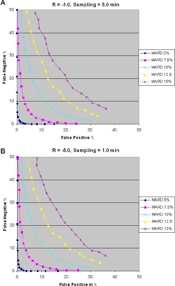
False positives vs false negatives with glucose rates of −1.0 (A) and −5.0 (B) mg/dl/min.

Next the effect of the sampling rate (sampling time) is discussed. The blood samples are not in sync with t_upper and t_lower of the “target area.” Results for a glucose rate of change of −1.0 mg/dl/min are shown in Figures 7 and 8. Results for glucose rates of change of −5.0 and −0.5 mg/dl/min are similar, but are not discussed here. The first thing to note is that there is a negative effect on false positives and false negatives when comparing Figure 7A to Figure 6A. This is because of the fact that in a real situation, and based on the initial glucose value, there is no guarantee that all patients' blood samples will hit the bottom edge of the “target area.” Some will hit beyond the bottom edge and will be considered false negatives. Figure 7A is a closer representation of the real world.

Figure 7.

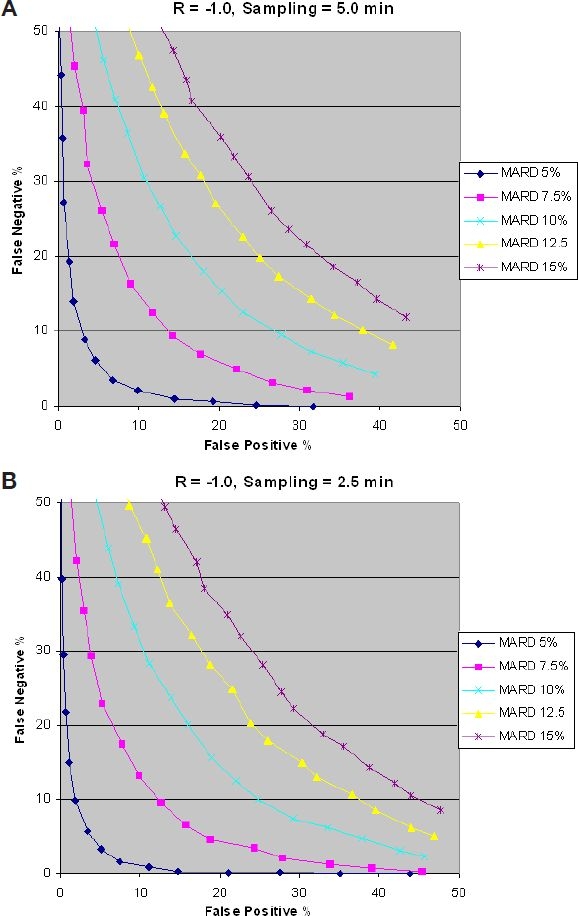
Effect of sampling time on false positives.

Figure 7 shows that increasing the sampling rate (reducing sampling time) beyond the critical sampling value increases the percentage of false positives. This can be explained by the fact that a faster sampling rate will increase the probability of intersecting the Hypo threshold level before t_lower, resulting in a false positive. In other words, results shown in Figure 7 suggest that a variable sampling rate is a better approach than a constant sampling rate. A slow sampling rate for a low glucose rate of change is more optimum and vice versa for a high glucose rate of change.

Figure 8B shows that reducing the sampling rate (increasing sampling time) increases the percentage of false negatives as compared to Figure 8A. This is explained by the fact that an increased sampling time increases the probability of reducing the number of hits in the “target area,” resulting in an increase of false negatives.

Figure 8.

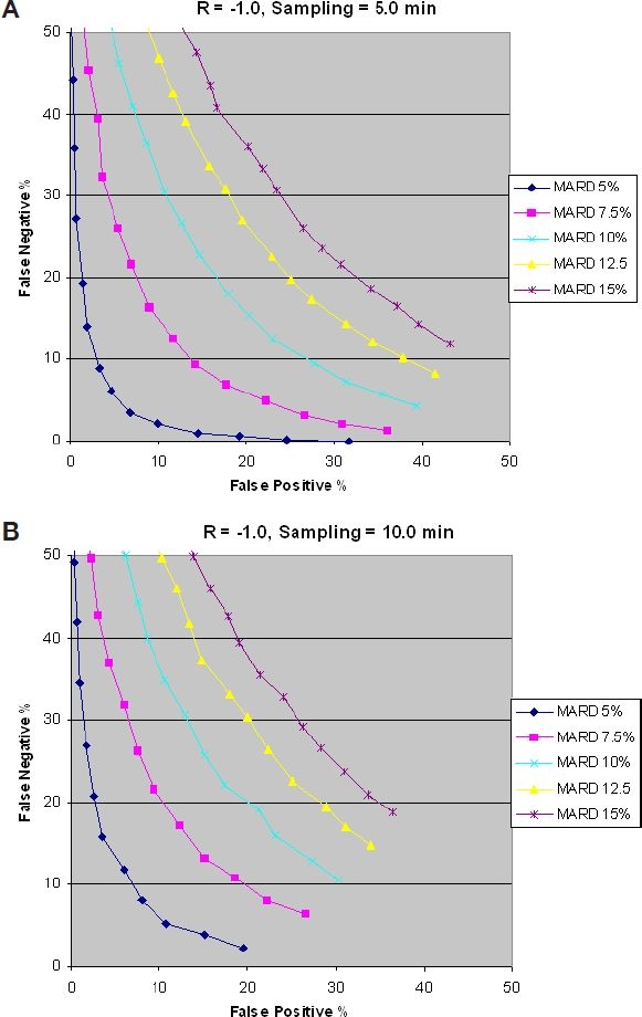
Impact of sampling time on false negatives.

Figures 7 and 8 show that for a given glucose rate of change, there is an optimum sampling rate (sampling time), a faster sampling rate from optimum increases the false positives, and a reduced sampling rate reduces the false positives while increasing the false negatives.

From Figures 5–8, we can conclude the following:

1. For a given glucose rate of change, there is an optimum sampling time.

2. The optimum sampling time as defined in the critical sampling rate section gives the best combination of low false positives and low false negatives.

3. There is a strong correlation between MARD and false positives and false negatives.

4. For false positives of <10% and false negatives of <5%, a MARD of <7.5% is needed.

Conclusions

A mathematical model has been developed to investigate the relationship between the accuracy of the continuous monitoring sensor as described by the MARD, and the number of false negatives and false positives as a function of blood glucose rate change is established. The following observations can be deduced from the mathematical derivations and the results obtained from running the simulator on N = 10,000 patients.

1. False positive and false negative ratios will vary depending on the alarm Hypo threshold set by the patient and the MARD value.

2. The sampling rate (number of hits in the “target area”) plays a key role in the number of false positives and false negatives. A variable sampling rate (slow sampling rate for slow blood glucose change and fast sampling rate for fast blood glucose change) provides lower false positives.

3. The sampling time is selected to be equal to the time base of the “target area” divided by 3.

4. To achieve a false positive ratio <10% and a false negative ratio of <5% requires an MARD of ≤7.5%.

5. There is a direct correlation between the MARD and the sensor accuracy. For a bias of zero, MARD is approximately equal to 0.8× the coefficient of variation. When the absolute of the relative bias is large compared to the coefficient of variation, the MARD is approximately equal to the absolute value of the relative bias.

6. When estimating the blood glucose rate of change using linear regression, the systematic relative bias in the estimated rate is equal to the systematic relative bias in the individual glucose measurements.

Abbreviations

Hypo

hypoglycemia

ISF

interstitial fluid

MARD

mean absolute relative difference

Appendix — Derivations

This appendix provides the technical derivations stated in the article. The notation and assumptions listed in the article are assumed in the derivation.

A.1 Estimation of the Glucose Rate of Change

Given noisy data $\left({\text{t}}_{\text{1}},\widehat{\text{G}}\left({\text{t}}_{\text{1}}\right)\right)$, …, $\left({\text{t}}_{\text{1}},\widehat{\text{G}}\left({\text{t}}_{\text{n}}\right)\right)$, it is desirable to estimate the blood glucose rate of change, $\text{bg}\widehat{\text{r}}$. Let g_i denote $\widehat{\text{G}}\left({\text{t}}_{\text{i}}\right)$. Standard linear regression yields the following estimate

$$bg\widehat{r}=\frac{{\displaystyle \sum \left(t_j-\overline{t}\right)}\times \left(g_j-\overline{g}\right)}{{\displaystyle \sum {\left(t_j-\overline{t}\right)}^2}}$$ (A.1.1)

One has

$$g_j-\left(1+\%b\right)\times G\left(t_j\right)+{\rho }_j$$ (A.1.2)

where ρ_j are independent normal random variables with mean 0 and variance ${\sigma }_{\text{j}}^{\text{2}}={\left(\%\text{cv}\times \text{G}\left({\text{t}}_{\text{j}}\right)\right)}^2$. Because it is assumed that the true blood glucose response is decreasing linearly with time at a rate bgr, one can write

$$G\left(t_j\right)=bgr\times t_j+C$$ (A.1.3)

for some intercept C. Equations (A.1.2) and (A.1.3) imply

$$\begin{array}{c}{\text{g}}_{\text{j}}-\overline{\text{g}}=\left(1+\%\text{b}\right)\times \text{bgr}\times {\text{t}}_{\text{j}}+\left(1+\%\text{b}\right)\times \text{C}+{\rho }_{\text{j}}-\left\{\left(1+\%\text{b}\right)\times \text{bgr}\times \overline{\text{t}}+\left(1+\%\text{b}\right)\times \text{C}+\overline{\rho }\right\}\\ =\left(1+\%b\right)\times bgr\times \left(t_j-\overline{t}\right)+\left({\rho }_j-\overline{\rho }\right)\end{array}$$ (A.1.4)

Substituting Equation (A.1.4) in Equation (A.1.1) yields

$$\begin{array}{l}\text{bg}\widehat{\text{r}}=\frac{{\displaystyle \sum \left({\text{t}}_{\text{j}}-\overline{\text{t}}\right)\times \left\{\left(1+\%\text{b}\right)\times \text{bgr}\times \left({\text{t}}_{\text{j}}-\overline{\text{t}}\right)+\left({\rho }_j-\overline{\rho }\right)\right\}}}{{\displaystyle \sum {\left({\text{t}}_{\text{j}}-\overline{\text{t}}\right)}^2}}\hfill \\ =\left(1+\%\text{b}\right)\times \text{bgr}\times \frac{{\displaystyle \sum {\left({\text{t}}_{\text{j}}-\overline{\text{t}}\right)}^2}}{{\displaystyle \sum {\left({\text{t}}_{\text{j}}-\overline{\text{t}}\right)}^2}}+\frac{{\displaystyle \sum \left({\text{t}}_{\text{j}}-\overline{\text{t}}\right)\times \left({\rho }_{\text{j}}-\overline{\rho }\right)}}{{{\displaystyle \sum \left({\text{t}}_{\text{j}}-\overline{\text{t}}\right)}}^2}\hfill \\ =\left(1+\%b\right)\times bgr+\frac{{\displaystyle \sum \left(t_j-\overline{t}\right)}\times \left({\rho }_j-\overline{\rho }\right)}{{{\displaystyle \sum \left(t_j-\overline{t}\right)}}^2}\hfill \end{array}$$ (A.1.5)

Because ρ_j are independent normal random variables with mean 0, the second term on the right-hand side of Equation (A.1.5) is normally distributed with mean 0. It remains to determine the variance of this term.

$$\begin{array}{l}\text{Var}\left(\frac{{\displaystyle \sum \left({\text{t}}_{\text{j}}-\overline{t}\right)}\times \left({\rho }_{\text{j}}-\overline{\rho }\right)}{{\displaystyle \sum {\left({\text{t}}_{\text{j}}-\overline{\text{t}}\right)}^2}}\right)=\text{E}{\left(\frac{{\displaystyle \sum \left({\text{t}}_{\text{j}}-\overline{\text{t}}\right)\times \left({\rho }_{\text{j}}-\overline{\rho }\right)}}{{{\displaystyle \sum \left({\text{t}}_{\text{j}}-\overline{\text{t}}\right)}}^2}\right)}^2\hfill \\ =\frac{\text{E}{\left\{{\displaystyle \sum \left({\text{t}}_{\text{j}}\times {\rho }_{\text{j}}\right)-\text{N}\times \overline{\text{t}}}\times \overline{\rho }\right\}}^2}{{\left({\displaystyle \sum {\left({\text{t}}_{\text{j}}-\overline{\text{t}}\right)}^2}\right)}^2}\hfill \end{array}$$

One has

$$=\frac{{\displaystyle {\sum }_i{\displaystyle {\sum }_j{t}_i\times t_j\times E\left({\rho }_i\times {\rho }_j\right)-2\times N\times \overline{t}}\times {\displaystyle \sum t_j\times E\left({\rho }_j\times \overline{\rho }\right)+N^2\times {\overline{t}}^2\times E\left({\overline{\rho }}^2\right)}}}{{\left({\displaystyle \sum {\left(t_j-\overline{t}\right)}^2}\right)}^2}$$ (A.1.6)

$$E\left({\rho }_i\times {\rho }_j\right)=\{\begin{array}{ll}{\sigma }_i^2\hfill & ifi=j\hfill \\ 0\hfill & otherwise\hfill \end{array}$$ (A.1.7)

$$\begin{array}{ll}\text{E}\left({\rho }_{\text{j}}\times \overline{\rho }\right)\hfill & =\frac{1}{\text{N}}{\displaystyle {\sum }_{\text{k}}\text{E}\left({\rho }_{\text{j}}\times {\rho }_{\text{k}}\right)}\hfill \\ \hfill & =\frac{{\sigma }_j^2}{N}\hfill \end{array}$$ (A.1.8)

$$\begin{array}{l}\text{E}\left({\overline{\rho }}^2\right)=\frac{1}{{\text{N}}^{\text{2}}}\times {\displaystyle {\sum }_{\text{j}}{\displaystyle {\sum }_{\text{k}}\text{E}\left({\rho }_{\text{j}}\times {\rho }_{\text{k}}\right)}}\\ =\frac{1}{N^2}\times {\displaystyle \sum {\sigma }_j^2}\end{array}$$ (A.1.9)

Substituting Equations (A.1.7)–(A.1.9) in Equation (A.1.6) results in

$$\begin{array}{l}\text{Var}\left(\frac{{\displaystyle \sum \left({\text{t}}_{\text{j}}-\overline{\text{t}}\right)\times \left({\rho }_{\text{j}}-\overline{\rho }\right)}}{{\displaystyle \sum {\left({\text{t}}_{\text{j}}-\overline{\text{t}}\right)}^2}}\right)\hfill \\ =\frac{{\displaystyle \sum \left({\text{t}}_{\text{j}}^{\text{2}}\times {\sigma }_{\text{j}}^{\text{2}}\right)-2\times \text{N}\times \overline{\text{t}}\times {\displaystyle \sum \left({\text{t}}_{\text{j}}\times \frac{{\sigma }_{\text{j}}^{\text{2}}}{\text{N}}\right)+{\text{N}}^2\times {\overline{\text{t}}}^{\text{2}}\times \frac{1}{{\text{N}}^{\text{2}}}\times {\displaystyle \sum {\sigma }_{\text{j}}^{\text{2}}}}}}{{\left({\displaystyle \sum {\left({\text{t}}_{\text{j}}-\overline{\text{t}}\right)}^2}\right)}^2}\hfill \\ =\frac{{\displaystyle \sum \left({\text{t}}_{\text{j}}^{\text{2}}\times {\sigma }_{\text{j}}^{\text{2}}\right)-2\times \overline{\text{t}}\times {\displaystyle \sum \left({\text{t}}_{\text{j}}\times {\sigma }_{\text{j}}^2\right)+{\overline{\text{t}}}^{\text{2}}\times {\displaystyle \sum {\sigma }_{\text{j}}^{\text{2}}}}}}{{\left({\displaystyle \sum {\left({\text{t}}_{\text{j}}-\overline{\text{t}}\right)}^2}\right)}^2}\hfill \\ =\frac{{\displaystyle \sum {\left(t_j-\overline{t}\right)}^2\times {\sigma }_{\text{j}}^2}}{{\left({\displaystyle \sum {\left({\text{t}}_{\text{j}}-\overline{\text{t}}\right)}^2}\right)}^2}\hfill \end{array}$$ (A.1.10)

Making the substitution ${\sigma }_{\text{j}}^{\text{2}}={\left(\%\text{cv}\times \text{G}\left({\text{t}}_{\text{j}}\right)\right)}^2$ in Equation (A.1.10) results in

$$Var\left(\frac{{\displaystyle \sum \left(t_j-\overline{t}\right)\times \left({\rho }_{\text{j}}-\overline{\rho }\right)}}{{\displaystyle \sum {\left(t_j-\overline{t}\right)}^2}}\right)={\left(\%cv\right)}^2\times \frac{{\displaystyle \sum {\left(t_j-\overline{t}\right)}^2\times G^2\left(t_j\right)}}{{\left({\displaystyle \sum {\left(t_j-\overline{t}\right)}^2}\right)}^2}$$ (A.1.11)

From Equation (A.1.3)

$$\begin{array}{l}{\text{G}}^2\left({\text{t}}_{\text{j}}\right)={\left(\text{bgr}\times {\text{t}}_{\text{j}}+\text{C}\right)}^2\hfill \\ ={\left(\text{bgr}\times \left({\text{t}}_{\text{j}}-\overline{\text{t}}\right)\text{+}\left(\text{bgr}\times \overline{\text{t}}+\text{C}\right)\right)}^2\hfill \\ =bg{r}^2\times {\left(t_j-\overline{t}\right)}^2+2\times bgr\times \left(bgr\times \overline{t}+C\right)\times \left(t_j-\overline{t}\right)+{\left(bgr\times \overline{t}+C\right)}^2\hfill \end{array}$$ (A.1.12)

Substituting Equation (A.1.12) in Equation (A.1.11) results in

$$\begin{array}{l}\text{Var}\left(\frac{{\displaystyle \sum \left({\text{t}}_{\text{j}}-\overline{\text{t}}\right)\times \left({\rho }_{\text{j}}-\overline{\rho }\right)}}{{\displaystyle \sum {\left({\text{t}}_{\text{j}}-\overline{\text{t}}\right)}^2}}\right)\hfill \\ ={\left(\frac{\%\text{cv}}{{\displaystyle \sum {\left({\text{t}}_{\text{j}}-\overline{\text{t}}\right)}^2}}\right)}^2\times \{{\text{bgr}}^2\times {\displaystyle \sum {\left({\text{t}}_{\text{j}}-\overline{\text{t}}\right)}^4+2\times \text{bgr}\times \left(\text{bgr}\times \text{t}+\text{c}\right)\times {\displaystyle \sum {\left({\text{t}}_{\text{j}}-\overline{\text{t}}\right)}^3}}\hfill \\ +{\left(bgr\times \overline{t}+C\right)}^2\times {\displaystyle \sum {\left({\text{t}}_j-\overline{\text{t}}\right)}^2}\}\hfill \end{array}$$ (A.1.13)

One notes that (bgr × t + C) is the true blood glucose level at the average time point.

Equation (A.1.13) simplifies when the observations are taken at equal time intervals Δt. Let t_j = j × Δt. Exploiting the moments of the discrete uniform distribution, one has

$$\begin{array}{ll}\overline{\text{t}}\hfill & \text{=}\frac{\text{N+1}}{\text{2}}\times \Delta \text{t}\hfill \\ {\displaystyle \sum {\left({\text{t}}_{\text{j}}-\overline{\text{t}}\right)}^2}\hfill & \text{=}\frac{{\text{N}}^{\text{2}}-\text{N}}{\text{12}}\times {\left(\Delta \text{t}\right)}^2\hfill \\ {\displaystyle \sum {\left({\text{t}}_{\text{j}}-\overline{\text{t}}\right)}^3}\hfill & =0\hfill \\ {\displaystyle \sum {\left({\text{t}}_{\text{j}}-\overline{\text{t}}\right)}^4}\hfill & =\frac{\left({\text{N}}^{\text{3}}-\text{N}\right)\times \left(3\times {\text{N}}^2-7\right)}{240}\times {\left(\Delta \text{t}\right)}^4\hfill \end{array}$$

Additionally,

$$\begin{array}{ll}\text{bgr}\times \overline{\text{t}}+\text{C}\hfill & =\frac{\text{G}\left({\text{t}}_{\text{l}}\right)+\text{G}\left({\text{t}}_{\text{n}}\right)}{\text{2}}\hfill \end{array}$$

Substituting into Equation (A.1.13) and simplifying results in the following expression for the variance:

$$\begin{array}{l}\text{Var}\left(\frac{{\displaystyle \sum \left({\text{t}}_{\text{j}}-\overline{\text{t}}\right)\times \left({\rho }_{\text{j}}-\overline{\rho }\right)}}{{\displaystyle \sum {\left({\text{t}}_{\text{j}}-\overline{\text{t}}\right)}^2}}\right)\hfill \\ =\frac{3\times {\left(\%\text{cv}\right)}^2}{N^3-N}\times \left\{\frac{\left(3\times N^2-7\right)}{5}\times {\left(bgr\right)}^2{\left(\frac{G\left(t_{\text{l}}\right)+G\left(t_{\text{n}}\right)}{\Delta t}\right)}^2\right\}\hfill \end{array}$$ (A.1.14)

A.2 Approximating the MARD

One has

$$\begin{array}{l}\text{MARD}=\frac{1}{\text{N}}{\displaystyle {\sum }_{\text{i}=1}^{\text{N}}\frac{\left|\widehat{\text{G}}\left({\text{t}}_{\text{i}}\right)\text{G}\left({\text{t}}_{\text{i}}\right)\right|}{\text{G}\left({\text{t}}_{\text{i}}\right)}}\hfill \\ =\frac{1}{\text{N}}\times {\displaystyle {\sum }_{\text{i}=1}^{\text{N}}\frac{\left|\text{G}\left({\text{t}}_{\text{i}}\right)\text{+}\%\text{b}\times \text{G}\left({\text{t}}_{\text{i}}\right)+\%\text{cv}\times \text{G}\left({\text{t}}_{\text{i}}\right)\times {\epsilon }_{\text{i}}-\text{G}\left({\text{t}}_{\text{i}}\right)\right|}{\text{G}\left({\text{t}}_{\text{i}}\right)}}\hfill \\ \text{=}\frac{1}{N}\times {\displaystyle {\sum }_{i=1}^N\left|\%\text{b}+\%cv\times {\epsilon }_{\text{i}}\right|}\hfill \end{array}$$ (A.2.1)

From the law of large numbers,

$$MARD\to E\left(|\%b+\%cv\times Z|\right)$$ (A.2.2)

where Z is a standard normal random variable. From symmetry one has

$$\text{E}\left(\left|\%\text{b}+\%\text{cv}\times \text{Z}\right|\right)=\text{E}\left(\left|-\%\text{b}-\%\text{cv}\times \text{Z}\right|\right)=\text{E}\left(\left|-\%\text{b}+\%\text{cv}\times \text{Z}\right|\right)=\text{E}\left(\left||\%\text{b}\right|+\%\text{cv}\times \text{Z|}\right)$$

If %cv = 0, then a direct consequence of Equation (A.2.1) is that = |%b|. Otherwise, let $\delta =\frac{|\%\text{b}|}{\%\text{cv}}$. Then

$$\begin{array}{ll}\text{E}\left(\left|\%\text{b}+\%\text{cv}\times \text{Z}\right|\right)& =\%\text{cv}\times \text{E}\left(\left|\delta +\text{Z}\right|\right)\\ & =\%\text{cv}\times \left\{{\displaystyle {\int }_{-\infty }^{-\delta }\left(-\delta -\text{z}\right)\times \varphi \left(\text{z}\right)\text{dz}+{\displaystyle {\int }_{-\delta }^{\infty }\left(\delta +\text{z}\right)\times \varphi \left(\text{z}\right)\text{dz}}}\right\}\\ & =\%\text{cv}\times \left\{{\displaystyle {\int }_{\delta }^{\infty }\left(-\delta +\text{z}\right)\times \varphi \left(\text{z}\right)\text{dz}+{\displaystyle {\int }_{-\delta }^{\infty }\left(\delta +\text{z}\right)\times \varphi \left(\text{z}\right)\text{dz}}}\right\}\\ & =\%\text{cv}\times \left\{{\displaystyle {\int }_{\delta }^{\infty }-\delta \times \varphi \left(\text{z}\right)\text{dz}+{\displaystyle {\int }_{-\delta }^{\infty }\delta \times \varphi \left(\text{z}\right)\text{dz}}}\right\}\\ & =\%\text{cv}\times \left\{{\displaystyle {\int }_{\delta }^{\infty }z\times \varphi \left(z\right)dz+{\displaystyle {\int }_{-\delta }^{\infty }z\times \varphi \left(z\right)dz}}\right\}\end{array}$$ (A.2.3)

The first term on the right-hand side of Equation (A.2.3) is equal to

$$\begin{array}{l}\begin{array}{ll}\%\text{cv}\times \left\{{\displaystyle {\int }_{\delta }^{\infty }-\delta \times \varphi \left(\text{z}\right)\text{dz}+{\displaystyle {\int }_{-\delta }^{\infty }\delta \times \varphi \left(\text{z}\right)\text{dz}}}\right\}\hfill & =\%\text{cv}\times \left\{-\delta \times \left(1-\Phi (\delta )\right)+\delta \times \left(1-\Phi \left(-\delta \right)\right)\right\}\hfill \\ \hfill & =\%\text{cv}\times \delta \times \left\{-1+\Phi (\delta )+1-\Phi \left(-\delta \right)\right\}\hfill \\ \hfill & =\%\text{cv}\times \delta \times \left\{\Phi (\delta )-\Phi \left(-\delta \right)\right\}\hfill \\ \hfill & =\%\text{cv}\times \delta \times \left(2\times \Phi (\delta )-1\right)\hfill \end{array}\hfill \\ \hfill =\left|\%\text{b}\right|\times \left(2\times \Phi \left(\frac{\left|\%\text{b}\right|}{\%cv}\right)-1\right)\hfill \end{array}$$ (A.2.4)

The second term on the right-hand side of Equation (A.2.3) is equal to

$$\begin{array}{l}\%\text{cv}\times \left\{{\displaystyle {\int }_{\delta }^{\infty }\text{z}\times \varphi \left(\text{z}\right)\text{dz}+{\displaystyle {\int }_{-\delta }^{\infty }\text{z}\times \varphi \left(\text{z}\right)\text{dz}}}\right\}\\ =\%\text{cv}\times \left\{{\displaystyle {\int }_{\delta }^{\infty }\text{z}\times \varphi \left(\text{z}\right)\text{dz}+{\displaystyle {\int }_{-\delta }^{\infty }\text{z}\times \varphi \left(\text{z}\right)\text{dz}}+{\displaystyle {\int }_{\delta }^{\infty }\text{z}\times \varphi \left(\text{z}\right)\text{dz}}}\right\}\\ \begin{array}{ll}\left(\text{letting\hspace{0.17em}t}=\frac{{\text{z}}^2}{\text{2}}\right)& \begin{array}{c}=\%\text{cv}\times 2\times {\displaystyle {\int }_{\delta }^{\infty }\text{z}\times \varphi \left(\text{z}\right)\text{dz}}\\ =\%\text{cv}\times \frac{2}{\sqrt{2\times \pi }}\times {\displaystyle \underset{\delta }{\overset{\infty }{\int }}\text{z}\times {\text{e}}^{\frac{{\text{z}}^{\text{2}}}{\text{2}}}\text{\hspace{0.17em}dz}}\\ =\%\text{cv}\times \sqrt{\frac{2}{\pi }}\times \frac{{\displaystyle {\int }_{{\delta }^2}^{\infty }{\text{e}}^{-1}\text{\hspace{0.17em}dt}}}{\text{2}}\\ =\%\text{cv}\times \sqrt{\frac{2}{\pi }}\times \exp \left(-\frac{{\delta }^2}{2}\right)\\ =\%cv\times \sqrt{\frac{2}{\pi }}\times \exp \left(-\frac{1}{2}\times {\left(\frac{\%b}{\%cv}\right)}^{\text{\hspace{0.17em}2}}\right)\end{array}\end{array}\end{array}$$ (A.2.5)

Combining Equations (A.2.2) through (A.2.5) yields

$$MARD\to |\%b|\times \left(2\times \Phi \left(\frac{|\%b|}{\%cv}\right)-1\right)+\%cv\times \sqrt{\frac{2}{\pi }\times \text{exp}\left(-\frac{1}{2}\times {\left(\frac{\%b}{\%cv}\right)}^2\right)}$$ (A.2.6)

The asymptotic limit of MARD can be used as an approximation. Equation (A.2.6) simplifies under two cases of interest.

Case 1: %b = 0.

$$\begin{array}{ll}\text{MARD}\hfill & \approx \text{|}0\text{|}\times \left(2\times \Phi \left(\frac{\left|0\right|}{\%\text{cv}}\right)-1\right)+\%\text{cv}\times \sqrt{\frac{2}{\pi }}\times \text{exp}\left(-\frac{1}{2}\times {\left(\frac{\%0}{\%\text{cv}}\right)}^2\right)\hfill \\ \hfill & =\%\text{cv}\times \sqrt{\frac{2}{\pi }}\hfill \\ \hfill & \approx 0.80\times \%\text{cv}\hfill \end{array}$$

Case 2: |%b|>>%cv

In this case, $\Phi \left(\frac{\text{|}\%\text{b|}}{\%\text{cv}}\right)\approx 1$ and $\text{exp\hspace{0.17em}}\left(-\frac{1}{2}\times {\left(\frac{\%\text{b}}{\%\text{cv}}\right)}^2\right)\approx 0$. Thus

$$\begin{array}{ll}\text{MARD}\hfill & \approx \text{|}\%\text{b|}\times \left(2\times \Phi \right)\left(\frac{|\%\text{b}|}{\%\text{cv}}-1\right)+\%\text{cv}\times \sqrt{\frac{2}{\pi }}\times \text{exp}\left(-\frac{1}{2}\times {\left(\frac{\%\text{b}}{\%\text{cv}}\right)}^2\right)\hfill \\ \hfill & \approx \text{|}\%\text{b|}\times \left(2\times 1-1\right)+\%\text{cv}\times \sqrt{\frac{2}{\pi }}\times 0\hfill \\ \hfill & =\text{|}\%\text{b|}\hfill \end{array}$$

A.3 Simulator Algorithm

1. 1. The simulator calculates t_upperand t_lower according to Equations (6A) and (6B)

   $${\text{t}}_{\text{upper}}=\frac{\text{Critical\hspace{0.17em}Threshold}-\text{G}\left({\text{t}}_{\text{l}}\right)}{\text{bgr}}$$ (A.3.1a)

   $${\text{t}}_{\text{lower}}=\frac{\text{Hypo\hspace{0.17em}Threshold}-\text{G}\left({\text{t}}_{\text{l}}\right)}{\text{bgr}}$$ (A.2.1b)
2. 2. The true glucose value is calculated at each time t_n using

   $$\text{G}\left({\text{t}}_{\text{n}}\right)=\text{G}\left({\text{t}}_{\text{l}}\right)+\text{bgr}\times {\text{t}}_{\text{n}},$$ (A.3.2)

   where G(t₁) is the initial glucose value.
3. 3. A standard normal random variable is generated with mean 0 and variance 1:

   $${\epsilon }_{\text{n}}=\text{norm}\left(0,1\right).$$ (A.3.3)
4. 4. The actual glucose measurement at time t_n is calculated by

   $$\widehat{\text{G}}\left({\text{t}}_{\text{n}}\right)=\text{G}\left({\text{t}}_{\text{n}}\right)+\%\text{b}\times \text{G}\left({\text{t}}_{\text{n}}\right)+\%\text{cv}\times \text{G}\left({\text{t}}_{\text{n}}\right)\times {\epsilon }_{\text{n}}.$$ (A.3.4)

5. 5. At every measurement time t_n the measured glucose value $\widehat{\text{G}}\left({\text{t}}_{\text{n}}\right)$ is compared to the alarm threshold. If $\widehat{\text{G}}\left({\text{t}}_{\text{n}}\right)$ ≤ Alarm Threshold, then the detection time t_alarm is given by t_n = t_n.

6. 6. If t_alarm > t_upper, add 1 to the false negative counter (FN).

7. 7. If t_alarm < t_lower, then add 1 to the false positive counter (FP).

8. 8. If not step 6 and not step 7, then add 1 to the true positive counter (TP).

9. 9. Steps 1 through 7 are repeated for the N patients, and the number of false positives and false negatives is accumulated.

10. 10. The percentage of false positives and false negatives is computed by dividing the counters FP and FN by N.

11. 11. MARD is calculated as

    $$MARD-\frac{1}{N}{\displaystyle {\sum }_{i=1}^N\frac{\left|\widehat{G}\left(t_i\right)G\left(t_i\right)\right|}{G\left(t_i\right)}}$$ (A.3.5)

References

- 1.Palerm CC, Willis JP, Desemone J, Bequette BW. Hypoglycemia prediction and detection using optimal estimation. Diabetes Technol Ther. 2005 Feb;7(1):3–14. doi: 10.1089/dia.2005.7.3. [DOI] [PubMed] [Google Scholar]
- 2.Bequette BW. Proceedings of the American Control Conference. Boston (MA): IEEE; 2004. Optimal estimation applications to continuous glucose monitoring; pp. 958–962. [Google Scholar]
- 3.Klonoff DC. A review of continuous glucose monitoring technology. Diabetes Technol Ther. 2005 Oct;7(5):770–775. doi: 10.1089/dia.2005.7.770. [DOI] [PubMed] [Google Scholar]
- 4.Kollman C, Wilson DM, Wysocki T, Tamborlane WV, Beck RW Diabetes Research in Children Network Study Group. Limitations of statistical measures of error in assessing the accuracy of continuous glucose sensors. Diabetes Technol Ther. 2005 Oct;7(5):665–672. doi: 10.1089/dia.2005.7.665. discussion 673-4. [DOI] [PMC free article] [PubMed] [Google Scholar]
- 5.Bode B, Gross K, Rikalo N, Schwartz S, Wahl T, Page C, Gross T, Mastrototaro J. Alarms based on real time sensor glucose values to alert patients to hypo- and hyperglycemia: the guardian continuous monitoring system. Diabetes Technol Ther. 2004 Apr;6(2):105–113. doi: 10.1089/152091504773731285. [DOI] [PubMed] [Google Scholar]
- 6.Tamada J, Eastman R, Desai S, Wei C, Lesho M. Hypoglycemia detection and prediction. Presented at the Third Diabetes Technology Meeting. 2003 Nov; San Francisco. [Google Scholar]
- 7.Kovatchev BP, Gonder-Frederick LA, Cox DJ, Clarke WL. Evaluating the accuracy of continuous glucose-monitoring sensors: continuous glucose-error grid analysis illustrated by TheraSense Freestyle Navigator data. Diabetes Care. 2004 Aug;27(8):1922–1928. doi: 10.2337/diacare.27.8.1922. [DOI] [PubMed] [Google Scholar]
- 8.Wentholt IM, Hoekstra JB, DeVries JH. A critical appraisal of the continuous glucose-error grid analysis. Diabetes Care. 2006 Aug;29(8):1805–1811. doi: 10.2337/dc06-0079. [DOI] [PubMed] [Google Scholar]
- 9.Hayter PG, Sharma M, Dunka L, Stout P, Price DA, Horwitz DL, Marhoul J, Vaez-Zadeh S. Performance standards for continuous glucose monitors. Diabetes Technol Ther. 2005 Oct;7(5):721–726. doi: 10.1089/dia.2005.7.721. [DOI] [PubMed] [Google Scholar]