Statistical Hypoglycemia Prediction

Abstract

Background

Hypoglycemia presents a significant risk for patients with insulin-dependent diabetes mellitus. We propose a predictive hypoglycemia detection algorithm that uses continuous glucose monitor (CGM) data with explicit certainty measures to enable early corrective action.

Method

The algorithm uses multiple statistical linear predictions with regression windows between 5 and 75 minutes and prediction horizons of 0 to 20 minutes. The regressions provide standard deviations, which are mapped to predictive error distributions using their averaged statistical correlation. These error distributions give confidence levels that the CGM reading will drop below a hypoglycemic threshold. An alarm is generated if the resultant probability of hypoglycemia from our predictions rises above an appropriate, user-settable value. This level trades off the positive predictive value against lead time and missed events.

Results

The algorithm was evaluated using data from 26 inpatient admissions of Navigator® 1-minute readings obtained as part of a DirecNet study. CGM readings were postprocessed to remove dropouts and calibrate against finger stick measurements. With a confidence threshold set to provide alarms that correspond to hypoglycemic events 60% of the time, our results were (1) a 23-minute mean lead time, (2) false positives averaging a lowest blood glucose value of 97 mg/dl, and (3) no missed hypoglycemic events, as defined by CGM readings. Using linearly interpolated FreeStyle capillary glucose readings to define hypoglycemic events provided (1) the lead time was 17 minutes, (2) the lowest mean glucose with false alarms was 100 mg/dl, and (3) no hypoglycemic events were missed.

Conclusion

Statistical linear prediction gives significant lead time before hypoglycemic events with an explicit, tunable trade-off between longer lead times and fewer missed events versus fewer false alarms.

Introduction

The Diabetes Control and Complications Trial¹ showed that glycemic control is critical in decreasing the severity of diabetic retinopathy, nephropathy, and neuropathy. However, the intensively treated group had a much higher incidence of severe hypoglycemia. Gabriely and Shamoon² concluded that improper insulin doses leading to hypoglycemic episodes increase the risk of severe morbidity or even death and may lead to the degradation of hypoglycemic awareness and responsiveness to future hypoglycemic episodes. Insulin therapy trades off the chronic high blood glucose consequences for the immediate dangers of hypoglycemia.

The dangers of hypoglycemia and the advent of continuous glucose monitors (CGMs) allow prediction/detection of hypoglycemia through CGM trend analysis, which could reduce the duration and severity of hypoglycemic episodes.

Biology-based patient models of diabetes can facilitate prediction by enabling simulation of blood glucose behavior from components such as insulin absorption, food ingestion, exercise, and patient-specific parameters.^3–7 We instead focus on simple statistical methods using only CGM data to predict/detect hypoglycemia. These methods require minimal sensors and patient input, making them more robust and potentially easier to implement commercially.

Early work on hypoglycemia prediction/detection analyzed daily patterns to identify high-risk times for hypoglycemia.⁸ Nguyen⁹ and Iaione and Marques¹⁰ detected hypoglycemia using an electrocardiogram and skin impedance. Palerm et al.¹¹ and DirecNet¹² not only detected but also predicted hypoglycemia from CGM data using optimal estimation and CGM built-in alarms, respectively. Choleau and colleagues¹³ took this further and implemented a simple prediction algorithm and food intervention to prevent hypoglycemia in rats. More recently, Sparacino et al.¹⁴ adapted this work to real blood glucose sensor data and used both linear and autoregressive models to state that hypoglycemia can be predicted 20–25 minutes in advance.

In this work, we extended the efforts of Sparacino et al.¹⁴ through the use of 1-minute data and by generating a hypoglycemic event-based predictive alarm. This alarm is intended to automatically shut off the insulin pump, thereby alleviating or avoiding the hypoglycemic event.

The use of statistical methods provides explicit certainty measures and enables a trade-off between lead time and positive predictive value. For example, when the alarm was set for an average of 26 minutes of lead time for hypoglycemic events, it missed no hypoglycemic events and generated false alarms only 30% of the time. Research by Buckingham and associates¹⁵ indicated that about 30 minutes of lead time is required to completely avert hypoglycemia. Less warning is less desirable, but still beneficial.

Continuous Glucose Monitor Data

Observational data comprise 26 data sets of 24 hours of 1-minute CGM readings from children with type 1 diabetes between 3 and 18 years old participating in a DirecNet study.¹⁶ Unfiltered, temperature-compensated, Navigator® data are accompanied by FreeStyle measurements, event logs, meal times, and carbohydrate content. Patients were admitted to clinical research centers after signing an informed consent. Some patients exercised for an hour on a treadmill in the afternoon and/or had their breakfast insulin bolus delayed for an hour. Data included 38,300 CGM measurements and 1347 finger stick measurements. It showed 21 hypoglycemic events (one or more successive glucose readings below 70mg/dl) determined by the sensor and 27 as determined by capillary glucose. Because the 1-minute readings of the Navigator are not calibrated, we calibrated the raw 1-minute sensor readings in each data set using a noncausal affine fit to the finger stick values.

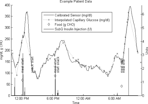
Figure 1 shows an example patient data set that illustrates the quality of data available and of calibration.

Figure 1.

Sample 24-hour patient data set. CHO, carbohydrate.

Metrics

We define our metrics in this section to explain how we quantify the performance of hypoglycemia prediction/ detection algorithms.

Different definitions of hypoglycemia have been proposed: Palerm et al.¹¹ use a threshold of 70 mg/dl; Nguyen⁹ uses a threshold of 60 mg/dl; Gabriely and Shamoon² define mild hypoglycemia as an episode that the patient can self-treat or a reading below 60 mg/dl; Miller et al.¹⁷ include cases where the patients reported typical symptoms; and the American Diabetes Association (ADA) working group on hypoglycemia in 2005 recommended a threshold of 70 mg/dl.¹⁸ We adhere to the ADA recommendations and declare readings below 70 mg/dl as hypoglycemic. CGM data and interpolated finger stick values provide two different reference measures of hypoglycemia.

Researchers assess predictive accuracy in different ways: Palerm and colleagues¹¹ use sensitivity and specificity on a minute-by-minute basis, whereas the DirecNet study group¹⁹ defines an alarm to be accurate if it occurs within ±30 minutes of hypoglycemia. Because the blood glucose readings and the effects of corrective actions are interdependent on a minute-by-minute basis, we follow DirecNet¹⁹ using event-based metrics.

Event Definitions

Corresponding to the predictive accuracy assessment of DirecNet, we define a hypoglycemic event as successive hypoglycemic reference measure readings below the hypoglycemic threshold (70 mg/dl). To prevent spurious hypoglycemic events, we require the reference value to rise above 75 mg/dl before we consider any subsequent events.

We define an alarm event as an alarm raised by a hypoglycemic prediction algorithm and the subsequent 120 minutes. This duration acknowledges the intended corrective action of turning the insulin infusion pump off for 90 to 120 minutes. Note that Buckingham and associates tested this strategy in a clinical trial.¹⁵ Additional alarms during the 120 minutes are ignored since they would be ignored in our proposed closed loop system.

Alarm Classification

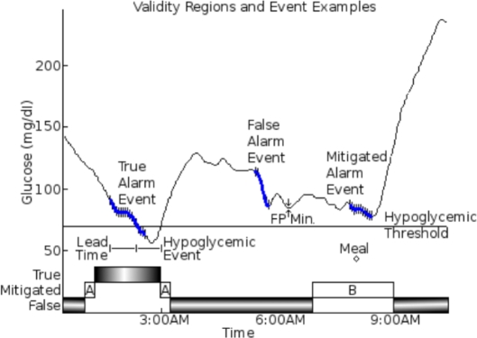
Figure 2 shows how we classify alarm events as true, mitigated, or false by when they occur relative to events. True alarm events occur during or up to 60 minutes before a hypoglycemic event.

Figure 2.

Example of true/false and mitigated temporal regions and alarm events. True alarm events start either during or up to 60 minutes before a hypoglycemic event. Type A-mitigated alarm events start where the lowest blood glucose reading in the next 60 minutes is above the hypoglycemic threshold but within 5 mg / dl. Type B-mitigated alarm events start up to 60 minutes before or 20 minutes after a meal. All alarm events that are not true or mitigated are false alarm events. The alarm events shown consist of a series of hypoglycemic alarms (vertical black lines) and a stretch of continuous alarming (thick, solid blue line) that links the hypoglycemic alarms. The continuous alarming connects consecutive hypoglycemic alarms that have no gaps larger than 15 minutes. The lead time for the true alarm event is the time difference between the start of continuous alarming and the start of the hypoglycemic event. The FP minimum for the false alarm event is the lowest reference glucose value within 60 minutes of the start of the false alarm event.

These metrics ignore nontrue alarm events when there is one of three types of mitigating factors. False alarm events within 80 minutes of the start of the data set, or within 60 minutes of the end of the data set, are ignored. If the minimum glucose level is above the hypoglycemic threshold but within 5 mg/dl of the hypoglycemic threshold, then we do not consider this a true event or a false event since it is within the glucose measurement error (this has been labeled as a type A mitigation in Figure 2). Alarm events where food intake or sensor failure occurred up to 60 minutes before or 20 minutes after the start of the alarm event are also considered inconclusive, labeled as type B mitigation in Figure 2.

False alarm events are all alarm events that are neither true nor mitigated.

Measured Quantities

The “true positive (TP) ratio” is the ratio of true alarm events to the total number of nonmitigated alarm events. The TP ratio refers to how often it was correct in predicting hypoglycemic events it alarmed for.

The “false positive (FP) minimum” measures the lowest glucose values up to 60 minutes after each false alarm event, i.e., how close the alarm was to being valid.

The “missed alarm ratio” is the percentage of hypoglycemic events that have no alarm events that overlap with them.

These metrics also report the “average lead time” between the start of continuous alarming and the start of hypoglycemic events. Here, continuous alarming refers to a stream of alarms where the maximum gap between alarms is less than 15 minutes (Table 1).

Table 1.

Definitions Summary

Events	Hypoglycemic event	Consecutive reference measure readings below 70 mg/dl
	Alarm event	The time at which an alarm is raised by a hypoglycemic prediction algorithm and the next 120 minutes. The starting alarm must not be in the 120-minute extension of a previous alarm event
Alarm event classification regions	True	The start is during or up to 60 minutes before a hypoglycemic event
	Mitigated	Not true, but the start is up to 60 minutes before a reading below 75 mg/dl (type A)
		or up to 60 minutes before or 20 minutes after a mitigating event (type B)
		or in the first 80 minutes of a data set
		or in the last 60 minutes of a data set
	False	All nontrue, nonmitigated regions
Metrics	True positive ratio	Number of true alarm events over number of nonmitigated alarm events
	False positive average minimum	Minimum value within 60 minutes of a false alarm event
	Lead time	Time between the threshold crossing and the start of the continuous alarming that overlap with a hypoglycemic event
	Missed event ratio	Number of hypoglycemic events with no associated true or false alarm events relative to the number of hypoglycemic events

Methods and Equations

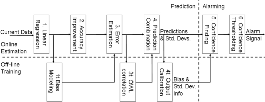
Figure 3 shows the steps in the statistical hypoglycemia algorithm. The steps are divided into three distinct sections. The online prediction steps transform real-time data into predictions of the future blood glucose values and estimates of the predictive accuracy. The online alarming steps convert the results of online prediction into a hypoglycemic alarm. The off-line prediction steps generate the empirical, statistical information used in the online steps from training data. We implemented this algorithm with discrete 1-minute time steps.

Figure 3.

Flowchart for statistical hypoglycemia algorithm. The process is divided into three sections. Online prediction steps are performed on real-time data to get predictions of the future blood glucose values and estimates of the predictive accuracy. Online alarming steps convert the results of online prediction into a hypoglycemic alarm. Off-line prediction training data are used to generate the empirical, statistical information used in the online steps.

The following equations and methodology are used for the steps just outlined.

Online Prediction

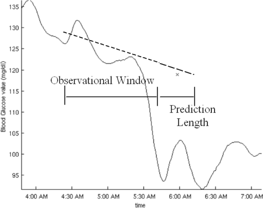
Input to the online prediction step is a history of realtime blood glucose data and empirical, statistical data from off-line training. Looking back several distances in time, we use lines fitted to real-time blood glucose data to generate one prediction of the future blood glucose trajectory for each distance. The distances we look back at are referred to as observational window lengths (OWLs, denoted mathematically as w); the distances forward that we predict are called prediction lengths (PLs, denoted mathematically as h) (Figure 4).

Figure 4.

An example of observational window length and prediction length with associated linear regression and linear prediction. The OWL is the time horizon back from now over which the regression is formed. The PL is the time horizon between now and the prediction.

The remaining steps use empirical, statistical data from the off-line prediction steps to remove prediction bias and harness extra information. Step 2 in Figure 3 improves the accuracy of all predictions for each PL and OWL, first by removing prediction bias against PL, OWL, and the standard deviation (SD) of the regression residuals and second, by harnessing the correlation between past, known residuals and the future, unknown prediction. Step 3 estimates the predictive accuracy for each PL and OWL using the PL, OWL, and SD of the regression residuals. Step 4 removes prediction bias versus OWL and PL, combines the predictions from different OWLs into one prediction per PL, and then removes any remaining prediction bias versus PL.

Linear Regression. We extrapolate lines fitted to current and past CGM values over the observational windows, g(τ) ∀τ∈ {t− w…t}, to estimate blood glucose trajectories, ĝ^t,W(t). The exponents w and t indicate that the estimated trajectories are calculated specifically for this time step, t, and this observational window length, w. (y) denotes that this quantity is a smooth function of time and is evaluated at time y. The line is fitted to recent glucose values by choosing the least-squares fit of an affine function in time:

$$\begin{array}{l}{\left[a^{t,w},b^{t,w}\right]}^{\text{T}}\equiv {\left[a,b\right]}^{\text{T}}\hspace{0.17em}s.t.\Vert A^w{[a,b]}^{\text{T}}-G^{t,w}\Vert =\underset{a,b}{\min }\Vert A^w{[a,b]}^{\text{T}}-G^{t,w}\Vert \\ {\left[a^{t,w},b^{t,w}\right]}^{\text{T}}={\left(A^{wT}{A}^w\right)}^{-1}{A}^{w\text{T}}{G}^{t,w}\end{array}$$

$$A^w\equiv {\left[\begin{array}{cccc}\hfill 0\hfill & \hfill -1\hfill & \hfill \dots \hfill & \hfill -w\hfill \\ \hfill 1\hfill & \hfill 1\hfill & \hfill \dots \hfill & \hfill 1\hfill \end{array}\right]}^{\text{T}}$$

$$G^{t,w}\equiv {\left[g(t),g(t-1),\dots g(t-w)\right]}^{\text{T}}.$$

We then use the time step and OWL-specific slope a^t,w, to estimate glucose values at PLs, h, in the future:

$${\widehat{g}}^{t,w}(t+h)=a^{t,w}h+g(t).$$

The result is a blood glucose prediction for each PL, h, OWL, w, and time step, t, where there were no sensor dropouts in the observational window.

Accuracy Improvement. The linear assumption does not reflect the true complexity of the blood glucose signal. For now, we mitigate this in two ways for each prediction. First, we use training data to remove the prediction residual bias versus PL, OWL, and SD of the regression residual. Second, we use known, past residuals and their off-line estimated covariance with the future prediction residual.

To use the off-line information, we first calculate the SD, σ^t,w, of the regression residuals, ${\overrightarrow{r}}^{t,w}$, for the current linear fits:

$${\sigma }^{t,w}\equiv \sqrt{\frac{1}{w+1}}\Vert {\overrightarrow{r}}^{t,w}\Vert$$

$${\overrightarrow{r}}^{t,w}\equiv g(t,\tau )-{\widehat{g}}^{t,w}(t+\tau )\forall \tau \in \left\{-w,-w+1,\dots 0\right\}.$$

We previously calculated the SDs for all possible line fits on training data. These SDs were sorted and grouped into 10 quality levels, ql. The mean SD for each quality level is denoted d^ql,w. For each quality level, we calculated the mean prediction residual bias for each PL, μ^ql,w(h), as well as the correlation coefficients between past and future prediction residuals, χ^ql,w. Using these, we can calculate a prediction improvement, Δ^ql,t,w(t + h), based on the PL, ql, and OWL:

$${\Delta }^{ql,t,w}(t+h)\equiv -{\mu }^{ql,w}(h)+{\chi }_{h,resids}^{ql,w}\hspace{0.17em}\hspace{0.17em}{\chi }_{resids,resids}^{ql,w}{\hspace{0.17em}}^{-1}({\overrightarrow{r}}^{t,w}-{\mu }^{h,ql,w}).$$

The first term removes the prediction residual bias, while the second term uses the correlation between the known regression residuals and the future prediction residual.

In practice, σ^t,w will fall between two quality levels, ql⁻, and ql⁺, such that d^ql−,w < σ^t,w < d^ql+,w. We consider σ^t,w a linear interpolation between the two means, with weights ρ^t,w and 1 − ρ^t,w:

$${\sigma }^{t,w}={\rho }^{t,w}{d}^{q{l}^{-},w}+(1-{\rho }^{t,w})d^{ql+,w}.$$

The improved prediction, ${\widehat{g}}_{imp}^{t,w}\left(t+h\right)$, is then the old prediction, ${\widehat{g}}^{t,w}\left(t+h\right)$, plus the weighted improvements:

$${\widehat{g}}_{imp}^{t,w}(t+h)\equiv {\widehat{g}}^{t,w}(t+h)+{\rho }^{t,w}{\Delta }^{q{l}^{-},t,w}(t+h)+(1-{\rho }^{t,w}){\Delta }^{q{l}^{+},t,w}(t+h).$$

Should σ^t,w fall outside the available means, d^ql,w, we use the improvement corresponding to the nearest one.

Error Estimation. For each quality level, we also calculate ${\widehat{\sigma }}^{ql,t,w}\left(t+h\right),$ the estimated SD for each PL, taking into account our knowledge of the regression residuals:

$${\widehat{\sigma }}^{ql,t,w}(t+h)\equiv {\chi }_{h,h}^{ql,w}-{\chi }_{h,resids}^{ql,w}\hspace{0.17em}\hspace{0.17em}{\chi }_{h,resids}^{ql,w}{\hspace{0.17em}}^{-1}{\chi }_{h,resids}^{ql,w}{\hspace{0.17em}}^{\text{T}}.$$

We use the same weights as in the previous section to get the standard deviation estimate for the specific σ^t,w:

$${\widehat{\sigma }}_{imp}^{t,w}(t+h)\equiv {\rho }^{t,w}{\widehat{\sigma }}^{q{l}^{-},t,w}(t+h)+(1-{\rho }^{t,w}){\widehat{\sigma }}^{q{l}^{+},t,w}(t+h).$$

Prediction Combination + Correction. At this stage, we have calculated a prediction, ${\widehat{g}}_{imp}^{t,w}\left(t+h\right)$ and SD,${\widehat{\sigma }}_{imp}^{t,w}\left(t+h\right)$, for each PL, time step, and sensor dropout-free OWL. We combine these into a single prediction, ${\widehat{g}}_{comb}^t\left(t+h\right)$, and estimated SD, ${\widehat{\sigma }}_{comb}^t\left(t+h\right)$, per PL using estimated covariance matrices, ${\widehat{\chi }}^t\left(t+h\right)$, and means, ${\widehat{\text{μ}}}^t\left(t+h\right)$, across all available OWLs.

The covariance matrix, $\widehat{\chi }\left(h\right)$, and mean prediction bias, $\widehat{\text{μ}}\left(h\right)$, were calculated off line for each PL using prediction residuals across OWLs normalized by their corresponding ${\widehat{\text{σ}}}_{imp}^{t,w}\left(t+h\right)$. To recover ${\widehat{\chi }}^t\left(t+h\right)$ and ${\widehat{\text{μ}}}^t\left(t+h\right)$ for the current time, we scale the elements of $\widehat{\chi }\left(h\right)$ and $\widehat{\text{μ}}\left(h\right)$ by the current ${\widehat{\sigma }}_{imp}^{t,w}\left(t+h\right)$ for each corresponding OWL:

$$\begin{array}{lll}{\widehat{\chi }}_{i,j}^t(t+h)\hfill & \equiv \hfill & {\overline{\chi }}_{i,j}(h){\widehat{\sigma }}^{t,w=i}(t+h){\widehat{\sigma }}^{t,w=j}(t+h)\hfill \\ {\widehat{\mu }}_i^t(t+h)\hfill & \equiv \hfill & \overline{\mu }(h){\widehat{\sigma }}^{t,w=i}(t+h).\hfill \end{array}$$

We then remove the prediction bias, ${\widehat{\text{μ}}}^t\left(t+h\right)$, from ${\widehat{g}}_{imp}^{t,w}\left(t+h\right)$ for each OWL and combine the results according to ${\widehat{\chi }}^t\left(t+h\right)$ to get ${\widehat{g}}_{comb}^t\left(t+h\right)$:

$$\begin{array}{ccc}{\widehat{g}}_{comb}^t(t+h)\hfill & \equiv \hfill & {\left({\overrightarrow{\mathbf{1}}}^T{\left[{\widehat{\chi }}^t(t+h)\right]}^{-1}\overrightarrow{\mathbf{1}}\right)}^{-1}{\overrightarrow{\mathbf{1}}}^{\text{T}}{\left[{\overrightarrow{\chi }}^t(t+h)\right]}^{-1}({\overrightarrow{\widehat{g}}}_{imp}^t-{\overrightarrow{\widehat{\mu }}}^t)\hfill \\ {\widehat{g}}_{imp}^t\hfill & \equiv \hfill & {\left[{\widehat{g}}_{imp}^{t,w=1}(t+h),{\widehat{g}}_{imp}^{t,w=2}(t+h),\dots ,{\widehat{g}}_{imp}^{t,w=w_{\max }}(t+h)\right]}^{\text{T}}.\hfill \end{array}$$

Here, $\overrightarrow{1}$ is a column vector of ones. The resultant uncertainty, ${\widehat{\text{σ}}}_{comb}^t\left(t+h\right)$, becomes

$${\widehat{\sigma }}^t{(t+h)}_{comb}\equiv {\left({\overrightarrow{\mathbf{1}}}^{\text{T}}{\left[{\widehat{\chi }}^t(t+h)\right]}^{-1}\overrightarrow{\mathbf{1}}\right)}^{-1}.$$

These equations provide more certainty when there are more sensor dropout-free OWLs available. Consequently, after a single sensor dropout, it takes as long as the shortest OWL to start predicting and as long as the longest OWL to regain complete predictive power.

Finally, we use training data to remove prediction biases for each PL and to calibrate the estimated SDs. We calibrate the resultant estimated SDs, ${\widehat{\text{σ}}}_{corr}^t\left(t+h\right)$, to be exact at the 75% confidence level. The 75% confidence level is midway between the two singularities of 50 and 100% confidence.

Similar to $\widehat{\chi }\left(h\right)$ and $\widehat{\text{μ}}\left(h\right)$ the prediction bias, ${\widehat{\text{μ}}}_{corr}\left(h\right)$, and SD scale factor, ${\overline{k}}_{corr}\left(h\right)$, were calculated using residuals normalized by ${\widehat{\sigma }}_{comb}^t\left(t+h\right)$. The corrected prediction, ${\widehat{g}}_{corr}^t\left(t+h\right)$, and estimated SD, ${\widehat{\sigma }}_{corr}^t\left(t+h\right)$, are

$$\begin{array}{ccc}{\widehat{g}}_{corr}^t(t+h)\hfill & \equiv \hfill & {\widehat{g}}_{comb}^t(t+h)-{\overline{\mu }}_{corr}(h){\widehat{\sigma }}_{comb}^t(t+h)\hfill \\ {\widehat{\sigma }}_{corr}^t(t+h)\hfill & \equiv \hfill & {\widehat{\sigma }}_{comb}^t(t+h){\overline{k}}_{corr}(h).\hfill \end{array}$$

Online Alarming

The alarming steps convert the predictions and error bounds into hypoglycemic alarms. We first generate probabilities of hypoglycemia, step 5 in Figure 3, and then threshold those probabilities and alarm, step 6 in Figure 3.

Confidence Finding. To relate the interdependent predictions and find an overall probability of hypoglycemia at any time during the total prediction horizon, we model the blood glucose behavior as a process, adding Gaussian noise between PLs:

$$g_{sim}(t+h_{i+1})\equiv g_{sim}(t+h_i)+N\left({\widehat{g}}^t(t+h_{i+1})-{\widehat{g}}^t(t+h_i),\sqrt{{\widehat{\sigma }}^t{\left(t+h_{i+1}\right)}^2-{\widehat{\sigma }}^t{\left(t+h_i\right)}^2}\right)$$

The Gaussian noise means and SDs are chosen so that the expected mean and SD match the predictions, ${\widehat{g}}_{corr}^t\left(t+h\right)$, and estimated SDs, ${\widehat{\sigma }}_{corr}^t\left(t+h\right)$. Using this model, we cannot analytically calculate the probability of hypoglycemia, so we simulate 500 trajectories. The ratio between the number of hypoglycemic trajectories and the total number of trajectories is then an estimate of the probability that the real trajectory will go hypoglycemic:

$${\widehat{P}}_{\text{hypoglycemia}}\equiv \frac{\#\text{hypoglycemic trajectories}}{\#\text{trajectories}}$$

Confidence Thresholding. We introduce a user-settable confidence threshold that allows real-time adjustment of the aggressiveness of the alarm. An alarm is triggered if the probability of hypoglycemia exceeds the confidence threshold.

Off-line Training

The algorithm harnesses the statistical properties of the various predictions to improve performance. These statistical properties are collected off line using training data. They are calculated in three distinct steps matching the online procedure. From linear regression we model the bias of our predictions. From error estimation we model the relation between predictions from different OWLs. From prediction combination we model the bias and error of the whole process.

Bias Modeling. We assess the accuracy of the linear regression-based predictions on training data. With this information, we first assign each regression to a quality level, ql, according to its SD. Here, each quality level has a mean SD of d^ql,w and contains a tenth of the training data.

Second, for the regressions in each quality level we calculate the mean, ${\overrightarrow{\text{μ}}}^{ql,w}$, and covariance, ${\overrightarrow{\text{χ}}}^{ql,w}$, of the past and future residuals, ${\overrightarrow{r}}_{comp}^{t,w}$:

$$\begin{array}{ll}{\overrightarrow{\mu }}^{ql,w}\equiv mean\left({\overrightarrow{r}}_{comp}^{t,w}\right)\hfill & \forall ts.t.\text{Quality}\left({\sigma }^{t,w}\right)=ql\hfill \\ {\overrightarrow{\chi }}^{ql,w}\equiv mean\left({\overrightarrow{r}}_{comp}^{t,w}{\left[{\overrightarrow{r}}_{comp}^{t,w}\right]}^{\text{T}}\right)\hfill & \forall ts.t.\text{Quality}\left({\sigma }^{t,w}\right)=ql\hfill \\ {\overrightarrow{r}}_{comp}^{t,w}\equiv g\left(t+\tau \right)-{\widehat{g}}^{t,w}(t+\tau )\hfill & \forall \tau \in \left\{-w,-w+1,\dots ,h_{\max }\right\}\hfill \end{array}.$$

The logical expressions on the right of the first two equations simply select cases matching the desired quality level.

Observational Window Length Correlation. To facilitate combining predictions for different OWLs, we use training data to determine the accuracy and correlation of results across OWLs. Since we already have estimated SDs, ${\widehat{\sigma }}_{imp}^{t,w}\left(t+h\right)$, we normalize the residuals by them before collecting them into covariance matrices, ⁻(h), and mean vectors, ⁻(h):

$$\begin{array}{ll}\overrightarrow{\mu }\left(h\right)\equiv mean\left({\overrightarrow{r}}^t\left(t+h\right)\right)\hfill & \forall t\hfill \\ \overrightarrow{\chi }(h)\equiv mean\left({\overrightarrow{r}}^t\left(t+h\right){\left[{\overrightarrow{r}}^t(t+h)\right]}^{\text{T}}\right)\hfill & \forall t\hfill \\ {\overrightarrow{r}}^t(t+h)\equiv \left({\widehat{g}}^{t,w}(t+h)-g(t+h)\right)/{\widehat{\sigma }}_{imp}^{t,w}(t+h)\hfill & \forall w\in \left\{w_{\text{min}},\dots ,w_{\text{max}}\right\}.\hfill \end{array}$$

Output Calibration. As a final correction we use training data to remove any remaining bias and misscaling of the estimated SDs. To find the prediction bias and corrective scale factor for ${\widehat{g}}_{comb}^t\left(t+h\right)$ and ${\widehat{\sigma }}_{comb}^t\left(t+h\right)$, we normalize the prediction residuals by ${\widehat{\sigma }}_{comb}^t\left(t+h\right)$. The mean prediction bias, ${\mu }_{corr}(h)$, is then

$${\mu }_{corr}(h)\equiv \text{mean}\left(\left[{\widehat{g}}_{comb}^t\left(t+h\right)-g\left(t+h\right)\right]/{\widehat{\sigma }}_{comb}^t(t+h)\right)\forall t.$$

For the correction factor, $k_{corr}(h)$, we use the 75th percentile of the normalized residual, correcting the 75% confidence level:

$$k_{corr}\left(h\right)\equiv as.t.a>\left|\left({\widehat{g}}_{comb}^t\left(t+h\right)-g\left(t+h\right)\right)/{\widehat{\sigma }}_{comb}^t\left(t+h\right)\right|in75\%ofcases$$

Results

The results shown here are trained on 13 of the insertions and validated on the other 13 insertions. We have chosen a representative split of the data sets.

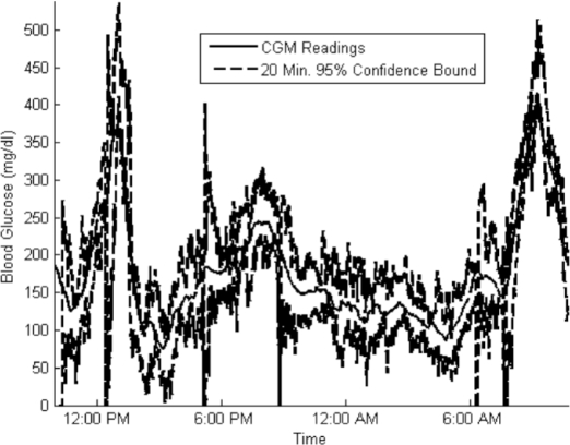
The alarm signal is generated using PLs of between 0 and 20 minutes and OWLs between 5 and 75 minutes. For PLs of 5, 10, 15, and 20 minutes, the 95% confidence bounds all contained 93, 94, 94, and 94%, respectively, of the CGM readings.

Interestingly, lead times far exceed the maximum prediction length of 20 minutes. This occurs because the prediction algorithm is trained over the full range of blood glucose values and does not model the autonomic response or user interventions that occur at low blood glucose values. As a result, predictions during descending, low blood sugar are consistently below true values. See Figure 5 for examples. This in turn causes the hypoglycemic alarm to trigger early. We expect to further improve results with more selective training and superior models in future research.

Figure 5.

Actual CGM readings and 95% confidence bounds on a 20-minute prediction for a sample patient admission. For validation data, 95% confidence bounds contained 93% of the CGM readings.

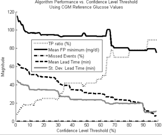
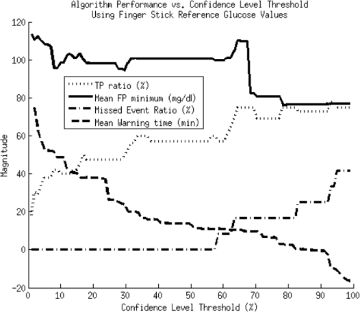
This algorithm has a tunable confidence threshold that determines how confident we need to be before triggering an alarm. We show result plots for two different reference glucose values, finger stick and CGM measurements (Figure 6 and 7).

Figure 6.

Performance metrics vs confidence level threshold using CGM readings as the reference blood glucose measure for determining when hypoglycemic events have occurred. No hypoglycemic events were missed.

Figure 7.

Performance metrics vs confidence level threshold using capillary glucose values as the reference blood glucose measure for determining when hypoglycemic events have occurred.

The plots in Figures 6 and 7 show two expected trends. First, with an increasing confidence level, there is a rise in the TP ratio and missed event ratio, with a concomitant drop in lead time, and FP minimum. This is consistent with what we expect since the higher the required confidence level, the more conservative the alarm algorithm. Because the alarm is more conservative, it both is less likely to alarm for dips that will not actually go hypoglycemic and will wait longer on real hypoglycemic events, thereby reducing the lead time.

Second, by using finger stick instead of CGM data as the reference measure, we see more missed alarms and lower maximum TP ratios for given lead times. This trend is a consequence of the disagreement between finger stick and CGM measurements. Finger stick measurements lead CGM measurements, causing them to dip further down and earlier during hypoglycemia, which both reduces lead time and potentially allows hypoglycemia to occur according to the finger stick values and not due to the CGM measurements. Also, the finger stick readings are infrequent and potentially miss hypoglycemic events caught by the more frequent CGM measurements.

The standard deviation of the lead time in Figure 6 is nearly as large as the average lead time itself. This is because some hypoglycemic events are characterized by a slow steady fall in blood glucose that makes them easy to predict, whereas others have sharp, quick drops that make them hard to predict. The lead times vary according to the difficulty of predicting the hypoglycemic event, giving a large lead-time variance. The average lead-time for the finger stick reference values was omitted because the errors in calibration overly distorted this metric.

Table 2 shows a small sample of the results from Figure 6 and 7 that we believe are representative values.

Table 2.

Results Summary

Confidence level (%)	Reference measure	TP ratio (%)	Mean lead time (min)	FP minimum (mg/dl)	Missed alarm event ratio (%)
64	Sensor	60	23	97	0
65	Sensor	70	23	100	0
93	Sensor	80	8.3	78	0
35	Finger stick	60	17	100	0
63	Finger stick	70	11	105	17
93	Finger stick	78	-9.3	77	33

Conclusion

Predictive alarming has the potential to allow corrective actions to mitigate and/or avoid hypoglycemia. We have shown a statistical algorithm that uses only blood glucose readings to predict and alarm before hypoglycemia occurs. Along with the algorithm, we have described a set of event-based metrics pertinent to hypoglycemic alarming.

The algorithm uses statistical methods to create predictions with error and confidence information. Statistical information obtained from training data improves the accuracy and removes residual bias. A user-settable minimum confidence level for the alarms provides a trade-off between true positive ratio vs lead time and missed events. This trade-off can be adjusted to match changing needs, such as greater lead during the day and more confidence during the evening.

Future work may allow for an improved training process by incorporating more complete models involving insulin, food, or exercise. We also plan to extend the algorithm to predict the severity of hypoglycemic events and predict more accurately in the presence of sensor dropouts. Using the existing model, our algorithm provides about a 23-minute lead time prior to a hypoglycemic event with a 70% TP ratio. We believe that this lead time can significantly benefit people with diabetes and help prevent dangerous hypoglycemic episodes.

Abbreviations

ADA

American Diabetes Association

CGM

continuous glucose monitor

FP

false positive

OWL

observational window length

PL

prediction length

SD

standard deviation

TP

true positive

Funding

Funding was made available from the Juvenile Diabetes Research Foundation.

References

- 1.The Diabetes Control and Complications Trial Research Group. The effect of intensive treatment of diabetes on the development and progression of long-term complications in insulin-dependent diabetes mellitus. N Engl J Med. 1993;329(14):977–986. doi: 10.1056/NEJM199309303291401. [DOI] [PubMed] [Google Scholar]
- 2.Gabriely I, Shamoon H. Hypoglycemia in diabetes: common, often unrecognized. Cleve Clin J Med. 2004;71(4):335–342. doi: 10.3949/ccjm.71.4.335. [DOI] [PubMed] [Google Scholar]
- 3.Parker R, Doyle FJ, 3rd, Peppas NA. A model-based algorithm for blood glucose control in type I diabetic patients. IEEE Trans Biomed Eng. 1999;46(2):148–157. doi: 10.1109/10.740877. [DOI] [PubMed] [Google Scholar]
- 4.Romero JS, Pastor FF, Payá A, Chamizo JG. Fuzzy logic-based modeling of the biological regulator of blood glucose. Lecture Notes Comput Sci. 2004;3066:835–840. [Google Scholar]
- 5.Karim EA. Neural network modeling and control of type I diabetes mellitus. Bioprocess Biosyst Eng. 2005;27:75–79. doi: 10.1007/s00449-004-0363-3. [DOI] [PubMed] [Google Scholar]
- 6.Santoso L, Mareels IM. Markovian framework for diabetes control. Proc 40th IEEE Conference on Decision and Control; Dec 2001. [Google Scholar]
- 7.Yamaguchi M, Kaseda C, Yamazaki K, Kobayashi M. Prediction of blood glucose level of type I diabetics using response surface methodology and data mining. Med Biol Eng Comput. 2006;44(6):451–457. doi: 10.1007/s11517-006-0049-x. [DOI] [PubMed] [Google Scholar]
- 8.Cavan DA, Hovorka R, Hejlesen OK, Andreassen S, Sönksen PH. Use of the DIAS model to predict unrecognised hypoglycaemia in patients with insulin-dependent diabetes. Comput Methods Programs Biomed. 1996;50(3):241–246. doi: 10.1016/0169-2607(96)01753-1. [DOI] [PubMed] [Google Scholar]
- 9.Nguyen HT. Neural-network detection of hypoglycemic episodes in children with type 1 diabetes using physiological parameters. Proceedings of the 28th IEEE Engineering in Medicine and Biology Society International Conference; 2006. [DOI] [PubMed] [Google Scholar]
- 10.Iaione F, Marques JL. Methodology for hypoglycaemia detection based on the processing analysis and classification of the electroencephalogram. Med Biol Eng Comput. 2005;43(4):501–507. doi: 10.1007/BF02344732. [DOI] [PubMed] [Google Scholar]
- 11.Palerm CC, Willis JP, Desemone J, Bequette BW. Hypoglycemia prediction and detection using optimal estimation. Diabetes Technol Ther. 2005;7(1):3–14. doi: 10.1089/dia.2005.7.3. [DOI] [PubMed] [Google Scholar]
- 12.Tsalikian E, Kollman C, Mauras N, Weinzimer S, Buckingham B, Xing D, Beck R, Ruedy K, Tamborlane W, Fiallo-Scharer R. Diabetes Research in Children Network (DirecNet) Study Group. GlucoWatch G2 Biographer alarm reliability during hypoglycemia in children. Diabetes Technol Ther. 2004;6(5):559–566. doi: 10.1089/dia.2004.6.559. [DOI] [PMC free article] [PubMed] [Google Scholar]
- 13.Choleau C, Dokladal P, Klein J, Ward WK, Wilson GS, Reach G. Prevention of hypoglycemia using risk assessment with a continuous glucose monitoring system. Diabetes. 2002;51(11):3263–3273. doi: 10.2337/diabetes.51.11.3263. [DOI] [PubMed] [Google Scholar]
- 14.Sparacino G, Zanderigo F, Corazza S, Maran A, Facchinetti A, Cobelli C. Glucose concentration can be predicted ahead in time from continuous glucose monitoring sensor. IEEE Trans Biomed Eng. 2007;54(5):931–937. doi: 10.1109/TBME.2006.889774. [DOI] [PubMed] [Google Scholar]
- 15.Buckingham BA, Cobry E, Clinton P, Gage V, Caswell K, Cameron F, Chase HP. Preventing hypoglycemia using predictive alarm algorithms and insulin pump suspension. Submitted to Diabetes Technology and Therapeutics; 2008 April; [DOI] [PMC free article] [PubMed] [Google Scholar]
- 16.Diabetes Research in Children Network (DirecNet) Study Group. Buckingham B, Beck RW, Tamborlane WV, Xing D, Kollman C, Fiallo-Scharer R, Mauras N, Ruedy KJ, Tansey M, Weinzimer SA, Wysocki T. Continuous glucose monitoring in children with type 1 diabetes. J Pediatr. 2007;151(4):388–393. doi: 10.1016/j.jpeds.2007.03.047. [DOI] [PMC free article] [PubMed] [Google Scholar]
- 17.Miller CD, Phillips LS, Ziemer DC, Gallina DL, Cook CB, El-Kebbi IM. Hypoglycemia in patients with type 2 diabetes mellitus. Arch Intern Med. 2001;161(13):1653–1659. doi: 10.1001/archinte.161.13.1653. [DOI] [PubMed] [Google Scholar]
- 18.Defining and reporting hypoglycemia in diabetes: a report from the American Diabetes Association Workgroup on Hypoglycemia. Diabetes Care. 2005;28(5):1245–1249. doi: 10.2337/diacare.28.5.1245. [DOI] [PubMed] [Google Scholar]
- 19.The Diabetes Research in Children Network (DirecNet) Study Group. Accuracy of the GlucoWatch G2 Biographer and the continuous glucose monitoring system during hypoglycemia: experience of the Diabetes Research in Children Network. Diabetes Care. 2004;27(3):722–726. doi: 10.2337/diacare.27.3.722. [DOI] [PMC free article] [PubMed] [Google Scholar]