Attentional Modulation of Adaptation in V4

Abstract

Adaptation and visual attention are two processes that alter neural responses to luminance contrast. Rapid contrast adaptation changes response size and dynamics at all stages of visual processing while visual attention has been shown to modulate both contrast gain and response gain in macaque extrastriate visual cortex. Since attention aims to enhance behaviorally relevant sensory responses while adaptation acts to attenuate neural activity, the question we asked is, how does attention alter adaptation? We present here single-unit recordings from V4 of two rhesus macaques performing a cued target detection task. The study was designed to characterize the effects of attention on the size and dynamics of a sequence of responses produced by a series of flashed oriented gratings parametric in luminance contrast. We found that the effect of attention on the response dynamics of V4 neurons is inconsistent with a mechanism that only alters the effective stimulus contrast, or only rescales the gain of the response. Instead, the action of attention modifies contrast gain early in the task, and modifies both response gain and contrast gain later in the task. We also show that responses to attended stimuli are more closely locked to the stimulus cycle than unattended responses, and that attended responses show less of the phase lag produced by adaptation than unattended responses. The phase advance generated by attention of the adapted responses suggests that the attentional gain control operates in some ways like a contrast gain control utilizing a neural measure of contrast to influence dynamics.

INTRODUCTION

Visual stimuli that rapidly change in luminance or contrast can activate rapid adaptation mechanisms that allow the retina and cortex to avoid saturation and preserve relative sensitivity (Shapley & Enroth-Cugell, 1986; Müller et al., 1999). Sequences of such stimuli, produced either by a scan path or by time-varying exogenous stimuli, will elicit sequences of responses that become progressively more attenuated and delayed (Motter, 2006). This rapid adaptation may, however, improve pattern discrimination (Müller et al., 1999) and render visual neurons more sensitive to changes in input statistics (Laughlin, 1981; Wark et al, 2009).

Attention, on the other hand, has a wide range of effects on the response properties of neurons in the visual cortex (reviewed in Reynolds and Heeger, 2009; Ghose, 2009). Different modes of attentional modulation can be demonstrated in macaque visual cortex depending on the type, number, size and spatial arrangement of visual elements in the task, the problem presented by the task and the strategy used to solve it, and the temporal structure of the behavioral trials (Ghose and Maunsell, 2002).

Two forms of response modulation, contrast gain (Reynolds et al., 2000) and response gain (Williford and Maunsell, 2006) appear to dominate under different conditions of task and strategy (Reynolds and Heeger, 2009; Ghose, 2009). Reynolds and Heeger (2009) propose that a normalization mechanism incorporates receptive field surround suppression into the strength of the divisive gain factor, and an attentional field that modifies both the stimulus and suppressive drives. Behavioral strategies that recruit surround suppression, coupled with visual stimuli that do not, increase sensitivity to low and intermediate contrasts (contrast gain). Larger visual stimuli that engage surround suppression, coupled with more narrowly focused deployments of attention, promote response gain. In another model (Ghose, 2009), the attentional field itself has a center-surround organization and depending on its tuning, and how it is positioned in visual space with respect to the sensory receptive field, attention can act by enhancing contrast gain, response gain or a combination of the two.

Thus, a growing consensus amongst investigators, reflected in the two models discussed above, holds that attention provides a flexible mechanism for enhancing neural activity from selected receptive fields that are encoding particular locations in space or features in a scene. The range of contrasts over which this enhancement occurs can depend on how the visual scene is constructed and the visually guided behavior interrogating that scene.

Real-world events worthy of attention often appear in sequences and develop over several seconds. Thus, attentional mechanisms must compete with changes in gain and dynamics in the feedforward pathways produced by rapid contrast adaptation. Here, we focus on this interaction, and show that attention counters some of the reduction in gain and phase distortion produced by adaptation. The phase lag produced by adaptation also allows us to show that attention produces a phase advance much like a contrast gain mechanism, lending support to the view that that attention utilizes a neural measure of contrast to adjust gain (Reynolds et al., 2000).

MATERIALS and METHODS

Behavioral Task

All animal-related procedures complied with National Institutes of Health guidelines and were approved by the Weill Cornell Medical College Institutional Animal Care and Use Committee. We recorded extracellularly from neurons in V4 of two male rhesus macaques (Macaca mulatta) performing a cued visual discrimination task. While the monkeys maintained central fixation, two circular grating patches flashed on a mean-luminance gray background. The monkeys released a bar when they detected a change in the contrast of either of the grating patches.

The structure of a single trial is illustrated in Figure 1. The monkey initiated a trial by fixating a central white cursor. After a short delay (50 ms), the grating patches appeared. The grating stimuli flashed on the screen with a temporal frequency of 2.087 Hz (46 frames per stimulus cycle at 96 frames per second) for the remainder of the trial. Another 40 ms after the grating patches first appeared, the fixation point changed color to cue the monkey as to which grating patch was the most likely to increase in contrast. The cue color indicated which stimulus was the likely target (blue indicated that the target would appear on the left, and yellow indicated that the target would appear on the right). Trials were run in blocks so that 12 trials in a row shared the same cue; blocking the cue resulted in the largest effect of the cue on animal behavior. Although initially the intent was to vary the cue randomly from trial-to-trial, pilot studies showed that the monkeys ignored the spatial cue with this approach. However, blocking trials resulted in a robust and consistent cueing effect, consistent with the selective allocation of attention to the cued stimulus. The cue predicted the location of the target in 95% of trials. Trials in which the cue correctly indicated the subsequent location of the target are called valid trials; trials in which the cue did not indicate the subsequent location of the target are called invalid trials. The block length and percentage of valid trials were chosen empirically to maximize the effect of the cue on the behavior of the animals.

Figure 1. Trial Layout.

(A) The temporal layout of a single experimental trial. First, a white fixation cursor appears. After the monkey fixates the cursor for 50 ms, two grating stimuli appear on the screen. The gratings flash at 2.1 Hz in an appearance-disappearance fashion for the duration of the trial. 40 ms after the initial appearance of the visual stimuli, the fixation cursor changes color to indicate that the trial has started. After a variable delay, one of the two grating stimuli increases in contrast. If the monkey releases a bar within 1 s of the target appearance, the monkey is rewarded.

(B) A typical example of the relationship between the visual stimuli, the fixation cursor, and the receptive field of a recorded neuron is shown. Blocks of 12 trials share the same cue, which is indicated by the color of the cursor. If the cursor becomes yellow, the left grating is most likely to be the target. If the cursor becomes blue, the right grating is most likely to be the target. The dotted red box indicates the receptive field of the neuron schematically; the boundary is not actually drawn on the screen. The size and location of the grating patch are those that elicit the largest response to a 100% contrast grating.

The target contrast step occurred between 1 and 4 seconds after the cue appeared; the target appearance coincided with the onset of the stimulus flash, and hence on an integer multiple of 479.2 (= 46/96) milliseconds. The first two flashes of the stimulus (“Period 1” and “Period 2”) never contained a target; all flashes that could be targets occurred during the “Target Period”. We base our analyses on these different stimulus periods to allow for the detection of time-varying response parameters arising from the action of contrast-gain adaptation processes.

The distribution of delay periods between the start of a trial and the appearance of the target approximated a discretely sampled exponential distribution; this choice was made to flatten the hazard function for the target contrast step (Luce, 1986), so as to maximally reward the animals for distributing their attention uniformly in time to the cued hemifield and grating during the “Target Period”. Under these conditions, the monkeys will typically adjust their attentional effort to be nearly constant (Ghose & Maunsell, 2002; Williford & Maunsell, 2006). In our study, the mean for the exponential distribution of delay times was 2.25 stimulus cycles, or 1.0781 seconds after the presentation of the second stimulus.

In our study, however, three factors made constructing a flat hazard function impossible: (1) no targets occurred with less than a 2 flash delay (958 ms); (2) targets only occurred at the onset of a stimulus flash, and hence were discretely distributed with corresponding peaks in the hazard function; and (3) the maximum target delay used was limited to 4 seconds, so that a peak in the hazard function just before the last possible target time was unavoidable (very few 4s trials were ever completed correctly, however, so this point may be less of an issue than the others).

Our analyses were designed to examine the variation of attentional effects with time and how attention interacts with adaptation. As described below, for every analysis where it was feasible, we considered the response to the grating stimuli as a function of cue and time. To parameterize the responses by time, we analyzed the response to the stimulus indexed by the presentation period: the first presentation of the stimulus is Period 1, the second presentation is Period 2, and subsequent presentations (when each stimulus could be a target) are the Target Period.

To complete a trial successfully, the monkey had to release a bar within 1 second after the contrast step occurred. All correctly completed trials were rewarded with a sip of juice, water, or diluted dietary supplement shake (Ensure, Abbott Laboratories, Abbott Park, IL), according to animal preference. Incorrect trials were followed by a 1 second “time-out” period in addition to the variable inter-trial interval of 500 – 750 ms. If three trials in a row were incorrect, the time-out increased to two seconds, and if five trials in a row were incorrect, the time-out increased to seven seconds.

A video eye tracker (Applied Science Laboratories, Bedford, MA) sampled the eye position at 120 Hz (approximately 8.3 ms per sample frame), with an accuracy of 0.5 degrees. High-frequency content of saccades extended up to approximately 100 Hz (Harris et al., 1990). When sampling at 120 Hz, high frequency content can be aliased downwards; in practice this means that we tended to overestimate the duration of the saccades, which made our estimates of fixation intervals conservative.

The horizontal and vertical eye positions were streamed to disk at 20 KHz. The system was calibrated on a daily basis to ensure accurate estimation of gaze position from gaze angle (see Supplemental Materials, 2 for more details). Each recording session began with the animal performing a fixation task. This simple fixation task with known fixation positions was used to build up a correspondence table between the eye tracker signal voltage and the corresponding eye positions onscreen. Eye positions that did not fall on the grid of points defined by the correspondence table were interpolated using a thin-plate approximating spline (Mazer & Gallant, 2003). Trials containing saccades or excessive noise due to a transient degradation in signal quality were marked as incorrect and not analyzed further. Thus, only trials in which the animals held fixation are included in these analyses (see Supplemental Materials 2 for more details).

Visual Stimuli

The contrast, orientation, spatial frequency, and size of the two sine-wave grating patch stimuli were the same, with one patch positioned within the receptive field of the neuron under study. Both stimuli initially appeared with the same contrast, flashed on the screen with an appearance-disappearance square wave temporal profile, and, after a variable delay, one stimulus increased its contrast. To span the range of a given neuron’s contrast response, five different initial Michelson contrasts were used: 4%, 8%, 16%, 32%, and 64%. We also included a blank stimulus to determine the neuron’s undriven activity level. The target stimulus to be detected was always the next highest contrast in the set, so that blank stepped to 4%, 8% stepped to 16%, etc. The 64% contrast stimulus stepped to 99% contrast, as by definition contrast cannot exceed 100%. Hence, for all but the blank and 64% stimuli, the target was twice the contrast of the preceding stimulus. This was intended to make the task equivalently difficult across the range of employed contrasts. The target was always an increasing contrast step to allow analysis of response transients to the target presentation (not presented in this report).

After a preliminary receptive field mapping with oriented bar stimuli, the location, orientation, size, and spatial frequency of a 100% contrast grating patch that maximally drove the neuron, and produced the best isolated single-unit waveform, were determined. Typical spatial frequencies used ranged from 0.8 to 1.5 cycles per degree, which corresponds with published data for spatial frequency tuning in V4 (Desimone & Schein, 1987; Gallant et al., 1996). These parameters were then used for the duration of the experiment, with the second stimulus placed symmetrically opposite the vertical meridian from the stimulus in the neuron’s receptive field. The spatial phase within each patch was randomized for each trial, to randomize the effects of subtle differences in eye position from trial to trial. The receptive fields for all neurons in this study fell in the ventral visual field with a typical eccentricity of 4 – 8 degrees of visual angle, consistent with recording locations in dorsal V4. As indicated above, grating patch size was chosen, along with a number of other parameters, to maximize the response of the isolated single-unit. Thus, an effort was made to reduce the contribution of the suppressive surround to the studied neural activity. Since the receptive field centers of V1 neurons dilate at lower contrasts (Sceniak et al., 1999), and our estimates of optimal stimulus size were made with 100% contrast gratings, the neural activity in this study was probably not influenced significantly by surround suppression.

Stimulus Generation System

A VSG 2/3 system (Cambridge Research Systems, Cambridge, UK) generated the visual stimuli using custom written software under real-time control of a second computer responsible for coordinating the behavioral protocol (TEMPO, Reflective Computing, St. Louis, MO). A 403.8 mm wide × 302.2 mm high CRT (Sony GDM-F520) presented the visual stimuli 57 cm from the monkey. The display resolution was 1024 by 768 pixels, running at a 96.0 Hz frame rate. The screen luminance at mean gray was 78cd/m² and the CRT output was linearized over its full range using the VSG gamma correction routines calibrated with the Opti-Cal system (Cambridge Research Systems). All visual stimuli were presented with the VSG in pseudo-12 bit mode to allow accurate presentations of gratings at 4% contrast. In addition to the communication with the behavioral control computer, four state bits from the VSG were streamed to disk at 20 KHz to accurately log the timing of the frame rate and to signal changes in the visual display.

Electrophysiologic Methods

In each animal, a craniotomy was centered on the lunate sulcus to provide chronic access to V4, as in Purpura et al. (2003). Briefly, a craniotomy was made with aseptic technique under gas anesthesia. A 19 mm inner diameter CILUX plastic cylinder (Crist Instrument Company, Inc., Hagerstown, MD) was positioned over the craniotomy with several titanium screws (Veterinary Orthopedic Implants, Inc., South Burlington, VT) around its base for support against sheer forces. The exposed skull and attached hardware were covered in dental acrylic (Ortho-Jet, Lang Dental Mfg Co., Inc., Wheeling, IL). A custom-made titanium socket was embedded in the dental acrylic, so that a post could lock the head in a stable position during recording sessions.

Craniotomy placement was chosen based upon a preoperative structural MRI with the monkey in the same stereotaxic frame used in the surgical procedure. The resulting structural images were compared against a standard rhesus macaque stereotaxic atlas (Paxinos et al., 1999) scaled to the size of the calvarium. The dorsal region of V4 on the lateral prelunate gyrus was the principal target for these studies, and the craniotomies were positioned to access a large region of dorsal V4. Post-operatively, either a structural MRI or CT with a tungsten microelectrode in situ confirmed craniotomy positioning over the prelunate gyrus. The location was confirmed as V4 by isolating neurons with receptive field sizes, locations, and response properties consistent with the known properties of V4 neurons (Desimone & Schein, 1987; Gattass et al., 1988; Gallant et al., 1996). Placement for both animals was further confirmed post hoc by gross anatomy and histology.

Sharp monopolar tungsten microelectrodes with epoxy insulation (FHC Inc, Bowdoin, ME; nominal impedance: 1.2-4 MOhm at 1 KHz) were used to record extracellular neuronal activity in these experiments. A plastic grid (Crist Instrument Company) inserted into the chamber provided a reproducible coordinate system for sub-millimeter consistency in electrode placement from day-to-day. A guide tube was used to penetrate the dura and provide mechanical stability. After insertion, the electrodes were advanced at least 1 millimeter beyond the tip of the guide tube using a modified hydraulic microdrive (Narashige International USA, East Meadow, NY), traveling tangentially down the anterior bank of the lunate sulcus. The electrode was connected to two optically isolated amplifier channels (TDT System 2, Tucker-Davis Technologies, Alachua, FL). One channel was high-pass filtered at 300 Hz for online detection of action potentials, while the other channel had no high-pass filtering. The channel with no high-pass filtering was streamed to disk and used for off-line spike isolation and analysis. Both channels were low-pass filtered at 7 KHz with a second-order Butterworth filter (12 dB per octave) to prevent aliasing of high frequency noise when sampled at 20 KHz.

Data Logging

Following amplification and filtering, the voltage signals from the amplifiers were sampled at 20 KHz using a 12-bit data acquisition card (NIDAQ-6071E, National Instruments Corporation, Austin, TX) and streamed to disk for later offline analysis. This data-streaming computer ran a custom-coded program for data logging in LabView (National Instruments) under Windows 2000 (Microsoft Corporation, Redmond, WA). This data-logging program simultaneously recorded the neuronal activity, the state of the visual stimulus generator, the voltage output of the infrared eye tracker, and the state of the behavioral control computer. This system allowed spikes to be clustered offline based upon size and waveform. We used an online waveform discriminator to perform the initial mapping of receptive fields with bars and gratings in real time under manual control. However, this online analysis was not used for any other purpose, as offline discrimination of activity was more reliable.

Spike Sorting

Our spike detection algorithm applied the nonlinear energy operator (NEO) of Kim & Kim (2000) to high-pass filtered voltage tracings to increase the signal to noise ratio of spikes for detection. (The NEO combines the frequency content and amplitude of the signal to give a single, scalar measure of the “spikiness” of the data, making spike detection substantially easier with fewer artifacts than a threshold applied directly to the high-pass filtered data.) The resulting measure was thresholded at 5 standard deviations above the mean, and the voltage peak nearest each threshold crossing was identified as a potential spike. Spikes were subsequently sorted using an algorithm based upon that proposed by Fee et al. (1996) with an additional principal components based dimensionality reduction step (Abeles & Goldstein, 1977). (See Supplementary Materials 1, for more information.)

Analytic Approaches

We developed several analytic approaches to maximize our ability to study the time-varying nature of neuronal responses given the data limitations present when working with an awake behaving animal. First, we parameterized the contrast response function in a standard fashion with a Naka-Rushton model. We also developed two other approaches to characterizing the response that offered more rapid convergence than traditional techniques for studying time-varying responses to periodic stimulation, namely local regression estimates of firing rates and harmonic stacking.

Contrast Response Function Model Fitting

We modeled a neuron’s response at time t_i with a thresholded energy model (Heeger, 1992) as:

$$f\left(t_i\right)=M+R_{\max }\frac{\max {\left(c\left(t_i\right)-T,0\right)}^2}{c_{50}^2+c{\left(t_i\right)}^2}$$ (1)

where f(t_i) is the firing rate of the neuron, c(t_i) is the contrast of the stimulus at time t_i, M is a parameter governing the undriven firing rate, R_max is the asymptotic high-contrast firing rate limit, c₅₀ is the contrast at which the response is 50% saturated (also known as the contrast gain), and T is a threshold. All nonlinear model fitting was performed by iteratively alternating Levenberg-Marquardt and Nelder-Mead algorithms until there was no improvement in the residual sum of squares. This process was repeated multiple times with random perturbations in the initial seed to avoid local minima, and the best performing model parameters were selected.

Other investigators (Williford & Maunsell, 2006; Reynolds et al., 2000) working in V4 have chosen to fit V4 responses with a Naka-Rushton type of model. The two models produce similar fits, and changes in the threshold in the above equation can result in effects that look very much like changes in the exponent of a Naka-Rushton model (Heeger, 1992). However, the strong suggestion of a threshold in some of our neuron’s responses, as in Figures 6 and 10, led us to adopt the thresholded energy model as a better fit to our data.

Figure 6. Example single unit CRF.

Spike count CRFs. Panels A-C (“Period 1”) contain the responses to the first stimulus presentation; panel A is the CRF when the stimulus is cued (“Attended”); panel B the CRF when the distractor stimulus is cued (”Unattended”), and panel C is the ratio of the Attended to the Unattended CRFs. The shaded area indicates the 95% confidence interval for the ratio as determined by 10,000 bootstrap replications.

Panels D-F (“Period 2”) contain the responses to the second stimulus presentation. Panel D is the Attended response, Panel E is the Unattended response, and F contains the ratio of panel D: panel E. Panel G plots the ratio of panel A to panel D, and Panel H plots the ratio of Panel B to panel E. Panels I-K (“Target Period”) contain the responses to all subsequent stimulus presentations. Targets could only appear in the “Target Period”. Panel I is the Attended response, Panel J is the Unattended response, and Panel K contains the ratio of panel I: panel J. Panel L plots the ratio of panel A to panel I, and Panel M plots the ratio of Panel B to Panel J.

Figure 10. Example F1 response magnitude.

The magnitudes of the F1 component of the responses are plotted as a function of contrast. Responses are separated into columns by attentional state and into rows by time period. The abscissa represents the stimulus contrast and the heavy black lines represent the magnitude of the F1 response (see text for calculation) to that stimulus contrast. Error bars are ± 2 jackknife standard errors. Panels G & H plot the ratio of the Period 1 to Period 2 responses, Panels L & M plot the ratio of the Period 1 to Target Period response, and Panels C, F, and K plot the ratio of the Attended to Unattended responses. Ratios of the F1 magnitudes are plotted on a log axis. Ratio plot 95% confidence regions are determined by 10,000 permutations of the two ratio populations.

An additional feature of the data captured by the thresholded energy model is the increase to a maximal firing rate before a decline to the asymptotic high contrast firing limit. This can be seen in the fit to the Period 1 attended condition, where the 32% contrast response appears larger than the 64% contrast response. While in this instance the difference appears to be within the variance of our measurements, similar effects were seen in multiple neurons, and examples can be seen in Figures 3 and 5 of Williford & Maunsell (2006). This strongly suggests that this feature of the responses of V4 neurons is real.

Figure 3. Accuracy by Contrast.

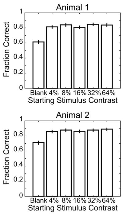
Each animal’s accuracy in trials where fixation was held is plotted as a function of stimulus contrast. Error bars indicate 95% confidence intervals. This figure is generated from the behavior during recording sessions for the neurons included in this report.

Figure 5. Population mean ring rates.

The mean firing rate response from 33 well-isolated single units recorded in V4 is shown. Each row of plots corresponds to a single stimulus contrast, indicated along the left margin. The left column contains the responses to Period 1, the center column to Period 2, and the right column to the Target Period. Firing rates are local regression estimates of the firing rate: the thick line indicates the mean attended firing rate, the thin line indicates the mean unattended firing rate, and the shaded region indicates the jackknifed 95% confidence limits for the unattended firing rate. The vertical scale is the normalized mean firing rate over the population.

Local Regression Estimates of Firing Rates

We treated the neuron’s firing behavior as a point process. In this view, a neuron’s firing probability is the marginal intensity function for that point process. The most common approach to estimate a time-varying marginal intensity function is the peristimulus time histogram. The peristimulus time histogram has relatively poor convergence properties when the marginal intensity varies rapidly, such as with initial response transients. This is because narrow bins must be used to capture rapidly varying signals. Narrow bins require a very large number of trials to provide a precise and accurate estimate of the marginal intensity function. Better estimates of the marginal intensity function can often be obtained by smoothing. Here we do this by generalizing the Parzen kernel-smoothing approach, which convolves spike times with a (usually Gaussian) kernel of fixed bandwidth to compute what is known as a spike density function (Levick & Zacks, 1970; Richmond et al, 1987; Schall et al., 1995; Szücs, 1998).

The Parzen kernel smoothing approach can be formulated more generally as a local likelihood regression problem (Loader, 1999). The local likelihood regression uses a low-order polynomial to approximate the marginal intensity function within a local neighborhood (a kernel function defines the size of the neighborhood). [The Parzen estimator, or spike density function, is the analytic solution when a constant is used as the approximating polynomial]. If the regression uses a linear or quadratic polynomial as the local approximation, similar convergence properties can be obtained with less bias at the extreme values of the density estimate for a given number of data points. We used a quadratic polynomial because curvature in the data can be exploited in the fitting while retaining a wider bandwidth reducing the variance in the resulting estimate. The local regression algorithms used are publicly available in the locfit library (Loader, 1999) and have been implemented in MATLAB as a part of the Chronux project (available for download at http://www.chronux.org). Our local regression estimates used a variable bandwidth that includes the larger of 150 nearest-neighbors’ spikes or 15% of the data, so regions of high firing rate had finer time resolution than those with low firing rates. We computed 95% confidence limits by jackknife, successively recomputing each estimate while leaving each trial out in turn.

Harmonic Stacking

Since our neuronal data were collected in response to periodic stimulation, we used a frequency-domain approach to quantify the response dynamics efficiently. In situations in which it is reasonable to assume that the response has reached a steady state (as it would in anesthetized, paralyzed preparations with extended stimulus presentations) the standard method of calculating Fourier components (e.g., Skottun et al., 1991) suffices. However, because of the limited duration of each period of interest here (~480 ms), and our desire to capture the dynamic effects of attention and adaptation, we did not want to make the steady-state assumption. We therefore used an approach that extends the standard Fourier components approach to these responses. Our particular approach was inspired by the “harmonic stacking” technique of Sornborger and coworkers (Sornborger et al., 2005) for analyzing optical imaging experiments.

We made the simplifying assumption that once an optimal orientation had been determined, the only parameters of the visual stimulus that affected the responses were the contrast of the stimulus and the stimulus period (whether the flash was the first, the second, etc., within a trial). That is, we ignored systematic dependence on the contrast presented on the previous trial (which is randomized) and variability due to the spatial phase of the grating stimulus (which was shuffled from trial-to-trial and further jittered by small differences in fixation position over trials). Analogously, we assumed that the only parameters of internal state that systematically affected the visual system were the attentional state (which we altered using the cue), the state of adaptation (which progressed across the duration of a trial), and the motivational state (reflected in the correct or incorrect performance of the trial). Other sources of variation were likely present, but we assumed that they were distributed randomly over all the trials.

To quantify the dynamics of the response that was time locked to the stimulus presentation for a particular set of parameters (cue, contrast, and stimulus period), we synthesized a signal from our data by first extracting the data segments from correct trials that have those parameters. Each of those segments, equal in duration to the inverse of the stimulation rate i.e. 1/2.087 Hz = 0.4792 seconds, was then placed head-to-tail, creating a synthetic time series by “cutting and pasting” individual segments of the data with identical parameters. The resulting synthetic time series could be considered “cyclostationary,” in that the same set of stimulus and internal state parameters governed the response on every presentation. We then calculated the Fourier components of this synthetic signal.

To calculate these Fourier components, we used the regression technique developed by Thomson (1982) to determine the best fitting sinusoid at each harmonic of the fundamental stimulation frequency. This multi-taper approach provides multiple independent estimates of the amplitude and phase of the sinusoid at each harmonic of the stimulus frequency. This approach is particularly advantageous because it does not require the spectrum of the spike train to be white. Confidence intervals for each component are determined by jackknifing the regression estimate over the trials (Thomson & Chave, 1991).

RESULTS

Behavioral Confirmation of Attentional Allocation

Cueing Effects on Performance Accuracy

We begin by demonstrating that spatial attention was linked to the cued target by showing that accuracy was higher in validly cued trials than in invalidly cued trials, as seen in humans performing a similar type of task (Posner, 1980). This was true in both animals. Animal 1 correctly completed 79.7% of validly cued trials (95% Confidence Interval, CI: 78.7% - 80.7%), and only 68.7% of invalidly cued trials (95% CI: 63.4% - 73.7%). Thus, the cue significantly altered Animal 1’s accuracy, with his accuracy on invalidly cued trials 11.0% lower than his performance on validly cued trials. Animal 2 completed 84.7% of validly cued trials (95% CI: 83.7% - 85.6%), and 73.1% of invalidly cued trials (95% CI: 67.6% - 78.2%). Hence, Animal 2 demonstrated a significant 11.5% drop in accuracy for invalidly cued trials, similar to Animal 1’s 11.0% performance accuracy drop, although Animal 2’s performance was better than Animal 1’s for both cue conditions. (Animal 2 broke fixation more frequently than Animal 1. If fixation breaks are scored as errors, the two monkeys’ accuracies are equivalent.)

In a 2-way linear ANOVA that includes the validity of the cue and the animal identity as factors, both factors exert a highly significant (P<0.001) effect on the performance accuracy; the interaction between animal cue and validity is borderline nonsignificant, with a P ~ 0.08. This result corroborates the above analysis: both animals made use of the cue to improve their performance on validly cued trials, and the two monkeys had different overall performance levels.

Cueing Effects on Reaction Time

We next present the reaction time distributions as further evidence that the cue modulated the animals’ allocation of spatial attention. In addition to effects on accuracy, cued target detection paradigms often show a decreased reaction time to a validly cued target (Posner, 1980). That is, correct responses to a validly cued target tend to be faster than responses to an invalidly cued target. This speeded response is often attributed either to a decrease in the difficulty of the task when uncertainty has been diminished, or to a cost paid for disengaging from the cued stimulus before responding to the uncued target (Posner, 1978). In humans, this difference in reaction time is often largest for simple tasks, and may decline below detection for difficult tasks (Posner, 1980).

Both animals showed an increased reaction time for invalidly cued correct trials (Figure 2). The shape of both reaction time distributions is roughly similar: nearly unimodal with a long tail. The qualifier ‘nearly’ is appropriate given that a second mode appears around 750 - 800 ms, especially for Animal 1, but also for Animal 2 in the invalid trials. This second mode corresponds to trials in which the animal missed the first appearance of the target, but detected the change with the subsequent flash and released the bar within the one-second reaction time window. As a result, of Animal 1’s secondary reaction time mode, the size of the tail depends on the animal, with Animal 2’s distribution biased to shorter reaction times than Animal 1. Correspondingly, while the median reaction time for the two distributions differs by only 8 ms, the mean reaction time for Animal 2 is 41 ms shorter than Animal 1.

Figure 2. Reaction Time Distributions by Cue Condition.

Data from correctly performed trials are plotted. Responses to validly cued trials are in the upper histogram, responses to invalidly cued trials are in the lower histogram. While Animal 1 does not show a significant shift in median reaction time (ΔRT_median = 10ms, P<0.46, Wilcoxon Rank Sum Test), Animal 2 shows a significantly slower reaction time in invalidly cued trials (ΔRT_median = 43 ms, P<0.001, Wilcoxon Rank Sum Test). This figure is generated from the behavior during recording sessions for the neurons included in this report.

We are safe in concluding that one of our animals completed validly cued trials faster than invalidly cued trials. Animal 2’s median reaction time for correct trials was 43 ms slower for invalidly cued trials, which is highly significant (P<0.001, Wilcoxon Rank Sum Test; one can also reject the hypothesis of equal distributions by a two-sample Kolmogorov-Smirnov test). The size of this cueing effect is comparable with those reported in the literature for humans and rhesus macaques performing similar tasks (Witte, et al., 1996). Animal 1’s median reaction time for correct trials is 10 ms slower for the invalidly cued trials, which is not significant (P<0.46, Wilcoxon Rank Sum Test).

Contrast Effects on Accuracy

Finally, we consider whether the effect of the cue was consistent over the range of contrasts employed in this study to see whether the attentional demands of the task changed with stimulus contrast. While response accuracy was largely unaffected by the contrast of the stimulus, as seen in Figure 3, both animals’ accuracy was significantly lower for trials that started with a blank stimulus and then transitioned to 4% contrast during the target period. The difference in performance appears to be due to the greater number of false alarms for the blank trials than for the trials that began with a visual stimulus. While for the nonblank trials the majority of errors (62.0% of the errors for Animal 1 and 58.2% of the errors for Animal 2) were misses, on blank trials only 39.2% of the errors for Animal 1 and 41.1% of the errors for Animal 2 were misses. This suggests that, at the eccentricities and sizes employed in this study, the 4% contrast target was near the animals’ behavioral threshold (here threshold is for the “average” contrast gain state of the animal after stimulation by the preceding trial of random contrast). However, part of this performance difference might be attributable to the greater temporal uncertainty in the blank trials. The animals’ accuracies on all other trials were nearly independent of contrast, with consistent fractions of misses and false alarms. This suggests that the animals’ strategies, and by extension, the attentional requirements of the task, were consistent over the range of contrasts employed in this study.

Electrophysiological Data

We recorded activity from 81 neurons in V4 from two animals. The data were first grouped by performance. Only correct trials were retained for analysis on the assumption that the animals’ motivational states were roughly comparable in these trials. At least six correctly performed repeats of each stimulus condition are required for successful application of the analytical methods described above. While a 10-repeat threshold is a more typical cutoff, the 6-repeat threshold was chosen because two units did not have at least 10 repeats for one stimulus-cue condition, despite having at least 10 repeats for the other 11 stimulus-cue conditions. In practice the 6-repeat threshold yielded tolerable error limits, with signal-to-noise ratios for the underrepresented conditions >= 2. However, omitting the two 6-repeat units from an analysis that included only units with >10 repeats did not substantially alter our conclusions. We recorded enough trials in all stimulus and cue combinations for 49 of these neurons. The typical dataset contained between 15 and 40 repeats of each stimulus in both cue conditions. Of these 49 neurons with sufficient trial numbers, 33 showed a clear visual response (spike count ANOVA with contrast as a factor is significant at a level P<.05). Only the data from these 33 visually responsive, well-isolated single units are presented in this report.

An example dataset for a single neuron is shown in Figure 4. The mean firing rates for correct trials are grouped according to the contrast of the stimulus and the time of the trial (“Period 1”, “Period 2”, or “Target Period”, as indicated in Figure 1). The timing of the stimulus cycle is indicated by the panels marked “On” and “Off” directly below the firing rate panels. Mean firing rates from trials in which the animal was cued towards the receptive field of the neuron (i.e., the “Attended” case) are indicated by the heavy black line; the mean firing rates from trials in which the animal was cued away from the receptive field of the neuron (i.e., the “Unattended” case) are indicated by the thin black line with the associated gray region indicating a 95% confidence interval computed by jackknife. As can be seen, this neuron is minimally responsive to the 4% contrast stimuli, but begins to develop a response to the 8% contrast stimulus. The 16% and 32% contrast stimuli show elevations in the mean of the firing rate in the attended case in the Period 1, Period 2, and Target Period responses. For the 64% contrast stimulus, however, the firing rate mean in the attended case exceeds the 95% confidence interval for the unattended case only for the Period 2 and Target Period responses. Note that the trend is for the difference to appear late in the response, while the trajectory of the initial transient is similar in both cue conditions. That is, it takes ~150 milliseconds for the significant cue-dependent differences in firing rate to appear in most of these conditions.

Figure 4. Example single unit ring rate response.

Correct trials are plotted from a well-isolated single unit recorded in V4. Each row of plots corresponds to a single stimulus contrast, indicated along the left margin. The left column contains responses from Period 1, the center column contains responses from Period 2, and the right column contains responses from the Target Period. Firing rates are calculated as local regression estimates: the thick line indicates the attended firing rate, the thin line indicates the unattended firing rate, and the shaded region indicates the jackknifed 95% confidence limits for the unattended firing rate. Vertical scale is in impulses per second (ips).

The population analog for Figure 4 is shown in Figure 5. The means of the firing rates are plotted by stimulus contrast (rows) and time period (columns), with the attended case indicated by the heavy line and the unattended case indicated by the thin line with 95% confidence limits shown as the shaded areas. Again, the population is minimally responsive to the Blank and 4% contrast stimuli. The population does show a response to the stimuli at 8 or 16% contrast, but it does not show an effect of cueing for these stimulus contrasts that exceeds the 95% confidence interval. Finally, there are clear responses to the 32% and 64% contrast stimuli that are accompanied by a significant cueing effect. Analogous with the single unit presented in Figure 4, the population shows more of an effect of the cue after the initial transient of the response.

Contrast response functions — Spike count

Several prior studies (Reynolds et al., 2000; Williford & Maunsell, 2006) have focused on the contrast response function (CRF) computed from the spike count in order to assess the effect of attention on firing rate in V4. We began this analysis with an approach inspired by these studies to quantify the effect of attention on our population of neurons. To compute our CRFs, we calculated the mean spike count at each contrast during each different cue condition and time period in the trial.

The results for the example neuron shown in Figure 4 are plotted in Figure 6. The two cue conditions are plotted in separate columns (headed by panels A and B), while the three time periods are plotted in separate rows (beginning with panels A, D, and I; recall that targets do not appear in the first two time-periods). Within each panel, the CRF is plotted as the number of spikes elicited by one cycle of the stimulus (0.4792 seconds in duration) as a function of increasing contrast. Error bars indicate 95% confidence limits on the mean spike count by jackknife. The smooth curves indicate the best fitting thresholded energy function for that condition. Comparing the Period 1 responses (Panels A and B), it can be seen that most of the difference between the CRFs is an increased response to the 32% contrast stimulus in the attended case. To facilitate the comparison, the ratio of the responses plotted in Panels A and B is shown in Panel C. Here, the point-by-point ratio of the mean response is indicated by the circles, the curve indicates the ratios of the respective fits, and the gray shaded area indicates the pointwise 95% confidence interval determined by 10,000 permutation shuffles of the two conditions. Hence, circles that fall outside of the shaded region indicate points at which the ratio exceeds what would be expected if the contrast response functions to the two attentional conditions were the same. Note that the only point in Panel C to fall outside of the 95% confidence range is at 32% contrast, in accordance with our visual assessment of the contrast response functions.

The Period 2 contrast response functions are shown in Panels D and E of Figure 6. Here there is a clear diminution in size of the unattended CRF compared both to the Period 2 attended case (Panel D) and to the Period 1 unattended case (Panel B). The ratio of the Period 2 attended to unattended CRFs is shown in Panel F. The Attended response (response to “Attended” stimuli) is ~50% larger than the Unattended response (response to “Unattended” stimuli) for all but the blank stimulus. The ratios of the Period 1 to Period 2 responses are shown in Panels G and H. Panel G illustrates that the only significant difference between the Period 1 and 2 Attended responses is an increase in the number of spikes in the 4% contrast case. Panel H indicates a decrease in response magnitude for the 8-64% contrast stimuli, with the decrease in the 32% and 64% response reaching point-wise significance.

In the Target Period, contrast adaptation and attention were likely to be approaching a steady-state — since the Target Period was always at least three periods into the stimulus presentation. The contrast response functions for the Target Period are shown in Panels I and J. In the attended case shown in panel I, the maximum firing rate is still approximately the same as in earlier periods, but the blank response has decreased and the 16% contrast response has increased, as illustrated in panel L. In the unattended case shown in panel J, the contrast response remains decreased relative to the Period 1 Unattended response, with the largest decrease occurring in the 64% contrast case, as illustrated in panel M. Finally, the cueing effect during the target period is illustrated in panel K, with no difference in the 4% and 8% responses, with the attended case showing a nonsignificant elevation of the 16% response, and a significant elevation of the 32% and 64% responses.

The fits plotted in Figure 6 (and Figure 10) were performed independently for the six sets of cue and stimulus period. However, it seems reasonable that certain parameters of the model might be the same across conditions, and might not change with the cue or with repeated presentations of the stimulus. Other parameters might be affected exclusively by the cue, or by the flash index. Following this intuition, we fitted the data from Figure 6 with 48 different potential candidate models, and used Mallow’s C_P (Mallows, 1973) to compare their performance objectively. For Mallow’s C_P, the goodness-of-fit is penalized by the number of free parameters in the model. Details of this analysis are presented in Supplemental Materials, 3.

Among the models we considered, the model with the single best C_P value for this neuron (C_P = 21.21) allowed R_max to vary independently between the six cue / period combinations, with the contrast gain determined by the cue (labeled R(q,f)c₅₀(q) in Table S1, Supplemental Materials, 3). This suggests that the six contrast responses are scaled versions of one another, shifted to the left or right by the cue. While this model has the best performance of those we considered, several models had nearly comparable performance by the C_P criterion: threshold independent (C_P = 22.88), contrast gain independent (C_P = 22.85), and response magnitude independent with threshold set by cue (C_P = 21.98). A different model-selection criterion, while regarding each of these models as “good” models for the data, might rank these models differently. (In this case, the ranking of their reduced χ² values —an alternative goodness-of-fit metric— agrees with the ranking of their C_P values, but in principle this might not be the case.) Nevertheless, all of these models represent substantial improvements over the common model (C_P = 39.17, with 4 free parameters), even though they each have 3-4 extra free parameters. These models also have significantly fewer parameters than the independent model, whose 16 parameters cause the goodness-of-fit measure to be heavily penalized (C_P = 31.00). The important point, however, is that all of the good models incorporate a shift in one of the nonlinear parameters of the model with attention: either the threshold or the contrast gain.

We applied our C_P analysis to all 33 neurons. No single model had a clearly best C_P, which suggests that the data did not constrain the model choices very tightly. The best models were tightly clustered with median C_P values slightly greater than 20. The two models with 5 parameters that performed well were: 1) contrast gain set by cue (c₅₀(q)); 2) response gain set by cue (R(q)). The models that had comparable performance mixed the contrast and response gain effects: R(f)c₅₀(q,f), R(q,f)c₅₀(q) and R(f)c₅₀(q). Those models appeared to be indistinguishable within the population, and bootstrap resampling of the C_P values showed that the confidence regions for the five best models all overlapped. It was difficult to distinguish a dominant model, particularly given the spread in the data, which appeared to be largest for the low-parameter models.

The common model, which fits all parameters simultaneously to the four cue and flash combinations, has 4 free parameters (see Table S1 in Supplemental Materials 3). The neurons for which the common model performed poorly were, in some sense, complicated (All four of the example neurons, Figures 4 and Supplemental Figures S4, S5 and S6 were from this class). For those neurons, essentially the same models that performed well in the population performed well, but mixed models were an improvement over the single effect models. That is, models that mixed response gain and contrast gain effects performed better. For those neurons, the two best 5 parameter models were still the contrast gain set by cue (c₅₀(q)) and response gain set by cue (R(q)); bootstrap resampling suggested that their median performance could not be distinguished (10,000 bootstrap resamplings of the difference between the median Cp values placed 0 at the 43.4^th percentile, for a one-tailed boostrap P = 0.434). The difference between the R(f)c₅₀(q) model and the c₅₀ (q) model was borderline significant (one-tailed bootstrap P = 0.047). The difference between the R(f)c₅₀(q) model and the R(q) model was not significant (bootstrap P = 0.151). The difference between the models with more than 5 parameters was not significant (bootstrap P = 0.32-0.84).

The low parameter models better described the neurons for which the common model performed well. However, even for those neurons, a mixed model, R(f)c₅₀(q) performed best. Its performance advantage over the common model was not significant enough to survive the bootstrapping procedure (P = 0.24). Inspection of these neurons suggested that the simple models were better for these neurons because the neurons had lower firing rates, and were therefore less well sampled. That is, the variance in the responses obscured any interesting adaptation or attentional effects that might have required several free parameters to accommodate. Despite this, two of these neurons were among those with a spike count that was significantly modulated by the cue.

The conclusion of Williford & Maunsell (2006) is a good one: several models can account for the effects of attention on the mean spike count contrast response functions. Their population-based argument was that the simplest explanation of the effects of attention on V4 responsiveness was a linear, multiplicative change. Note also that, of the 5 parameter models listed in Table S1 (Supplemental Materials, 3), the R(q) model has the best C_P, arguing that if you restrict attention to affect a single parameter, the best choice is R_max.

However, our analysis is fundamentally different than Williford and Maunsell’s in two respects. Their analysis did not allow for any mixed models that could combine effects, and their approach combined responses to repeated, randomly spaced presentations of stimuli, averaging temporal adaptation effects in with cueing effects. By modeling the temporal evolution of the response, and allowing mixed linear-nonlinear effects, our analysis indicates that single neurons can demonstrate changes of their contrast response functions with attention that can best be described as a mixed effects of response gain and contrast gain.

Because the ratio plots in Figures 6 and 10 are intended as exploratory devices to allow detection of point-wise differences between CRFs of two conditions (time period or cue), they do not correct for multiple comparisons. The 7 ratio plots each have 6 points in them, each of which has a 5% chance of falling outside of the confidence interval due to chance alone; hence we would expect ~2 points total from all of the ratio plots to fall outside of the confidence intervals due to chance alone. However, this neuron showed 13 points outside of the confidence limits, well above what would be expected by chance. As a more rigorous control for multiple comparisons that assess the significance of modulation effects due to the cue and time period, we performed a three-way ANOVA that includes the stimulus contrast, cue, and time-period as factors. This analysis confirms that the mean spike count is significantly modulated by the contrast of the stimulus (P < 0.001) and the cue (P < 0.002), but not time period (P > 0.12). This agrees with our qualitative assessment of the firing rate behavior, where contrast and attention both dramatically alter the firing patterns of the neuron. The time period effect did not reach significance, which can be attributed to the relative lack of an effect in the attended case.

Figure 7 shows the population average contrast response functions plotted by condition and time period, as in Figure 6. The shaded gray areas indicate the point-wise 95% confidence interval for the population means. As was suggested in the population mean firing rate data shown in Figure 5, the ratio plots show significant differences in the ratios of attended to unattended spike counts for the 32% and 64% contrast stimuli, with the magnitude of the attentional effect trending towards higher values over the course of the trial. The attentional enhancement of the population mean response to the 32% contrast stimulus is 24.4% during Period 1, increasing to 27.1% during Period 2 and 29.8% during the Target Period. The attentional enhancement of the population mean response to the 64% contrast stimulus is 22.4% during Period 1, increasing to 30.5% during Period 2 and 37.9% during the Target Period.

Figure 7. Population Spike Count CRF.

The population mean contrast response functions are separated into columns by attentional state and into rows by time period. The abscissa represents the stimulus contrast and the lines represent the normalized mean spike count in response to that contrast. Confidence intervals are ± 2 jackknife standard errors. Panels G & H plot the ratio of the Period 1to Period 2 responses, Panels L & M plot the ratio of the Period 1 to Target Period response, and Panels C, F, and K plot the ratio of the Attended to Unattended responses. Ratios of the CRFs are plotted on a linear axis. Confidence intervals are ±2 jackknife standard errors of the mean.

The data from all 33 neurons were each subjected to a three-way ANOVA that included the stimulus contrast, cue, and time period as factors (see Table 1). The mean spike count was significantly modulated by the contrast of the stimulus for 93% of the neurons, with the two neurons that were are not significantly modulated by contrast just missing the significance criterion (both are P < 0.10). The cue was a significant factor for slightly less than half (42%) of the neurons, while the stimulus period was a significant factor for 21% of the neurons. The fraction of neurons whose response size was significantly affected by cue is comparable to the 37% reported by Williford & Maunsell (2006) and the 46% reported by Reynolds, et al. (2000). However, as we will see below, the fraction of neurons whose response dynamics were affected by cue or time period is a much larger number.

Table 1.

	Contrast	Cue	Stimulus Period
Spike Count	31/33 (93.4%)	14/33 (42.4%)	7/33 (21.2%)
F1	33/33 (100%)	27/33 (81.8%)	32/33 (97.0%)

Response gain and contrast gain across the trial

If we restrict the curve fitting of Eq. 1 to the CRFs of each time-period (Period1, Period 2, and Target Period) in isolation with all 16 parameters fit independently for each cue condition and time-period, we can examine the progress of contrast gain and response gain across the trials. In Figure 8A, the mean and 95% confidence intervals (extrapolated from standard errors calculated by jackknife) are shown for ratios of C50 values across the three time-periods. The ratios are formed from the C50 parameter fits for the Unattended responses (numerator) and the Attended responses (denominator). Since C50 is the value of luminance contrast for which the CRF has attained 50% of its maximum value, a ratio of greater than 1 indicates that C50 Unattended is at higher contrast values than C50 Attended; the corresponding CRF for Attended responses is shifted to lower contrasts than the CRF for the Unattended responses. A ratio of 1 would imply that the CRFs for the unattended and attended data are not shifted along the contrast axis with respect to each other. For Figure 8A, the C50 ratios in Period 1 have a range of values that do not include the value of 1. The 95% confidence interval does include 1 for Period 2, but the ratios for the Target Period are again significantly different from 1. Thus, contrast gain appears to be a significant factor influencing neural responses during Period 1, less so in Period 2 and becomes a stronger influence again in the Target Period.

Figure 8. Progression of contrast gain and response gain across the stimulus cycles of the task.

(A) Ratios of C50 values across three stimulus cycles, Period 1 (left), Period 2 (middle), Target Period (right). The C50 values were obtained by fitting the CRFs with Eq. 1 with all parameters restricted to fit each condition of time-period and attentional cue separately. The ratio is formed between the C50 values for the Unattended responses and the values for the Attended responses. The mean ratio is plotted for each stimulus cycle (time-period) as is the 95% confidence interval for the mean.

(B) Ratios of Rmax values across three stimulus cycles. The Rmax values were obtained by separate fits of Eq. 1 to each time-period and cue condition. For each neuron, the Rmax value for the Eq. 1 fit to the Unattended CRF is divided by the Rmax value for the Eq. 1 fit to the Attended CRF. The mean of the ratios for all the neurons and the 95% confidence interval for the mean are plotted for Period 1 (left), Period 2 (middle) and Target Period (right).

In Figure 8B, ratios of the fitted parameter values for Rmax are plotted for the three time periods. Here, the ratio of Rmax Unattended to Rmax Attended is a measure of the strength of the response gain introduced by attention. If the Rmax ratio is 1, then the Rmax for the CRF of the Unattended responses is equivalent to that of the CRF for the Attended responses and hence response gain would not be considered a significant factor. On the other hand, an Rmax ratio less than 1 would indicate that Rmax Attended is larger than Rmax Unattended implying that response gain plays a significant role in shaping those responses. For Figure 8B, the 95% confidence interval for the Rmax ratios from Period 1 brackets the value of 1 indicating that response gain is probably not a significant factor as the trials begin. However, Rmax ratios significantly less than 1 are seen for Period 2 and the Target Period. Thus, the conclusions we can make from Figure 8 are that as a trial begins, attention modulates contrast gain, but that by the second flash (Period 2), response gain dominates. Finally, during the following Target Period, attention modulates both contrast gain and response gain.

Quantifying Cue Effects on Response Dynamics

While the spike count measures show significant modulation with attention, this is not uniform over the entire response interval of 480 ms. As discussed in the initial presentation of Figure 5, the populations’ initial response transients tend to be the same regardless of the cue, with the attentional effect emerging later during the sustained component of the response. This later emergence of the attentional effect was previously mentioned by Reynolds et al. (2000), but not analyzed in detail. To analyze this aspect of the effect of attention on the firing rate dynamics, we developed a method analogous to the computation of the Fourier components used with steady-state stimulation (see Methods: Harmonic Stacking). We focus in this report on the analog of the first Fourier component of the response, which we call the F1 component. The F1 component is a complex number that represents the magnitude and phase of the best fitting sinusoid with a frequency identical to the fundamental stimulation frequency used for these experiments (i.e., 2.087 Hz). Similar results were obtained with higher-order harmonics, F2, F3, F4 and F5 and the sum of the higher-order odd harmonics (Hudson et al., 2005). The F1 component captured most of the power in the response waveform so it was used as the measure to summarize the response characteristics in our analysis of dynamics.

The F1 components for the example neuron are plotted in the complex plane in Figure 9. Panels A-C show responses in Period 1, Period 2, and the Target Period, respectively. For each period, each of which represents a different sample from the time-evolving attentional and adaptation processes shaping the neural responses in these trials, the contrast response function is shown as a trajectory in which the distance from the origin indicates the magnitude of the best fitting sinusoid, and its phase as the angle from the positive x-axis. The attended condition is plotted in black, the unattended condition in gray. The ellipsoids represent 95% confidence limits as determined by bootstrapping over trials (10,000 replications). For the first stimulus period (Panel A), the trajectories are nearly overlapping; they are progressively more separated in subsequent periods (Panels B and C), especially at the higher contrasts. Note that as the responses progress from Panels A and B to C, the trajectories of the contrast response functions in the complex plane tilt closer to the left side of the real axis; the responses all develop more phase lag as contrast adaptation increases into the Target Period. At 64% contrast in the Target Period, the phase of the Unattended responses (gray) are at a larger phase angle than the phase of the Attended responses (black).

Figure 9. Example of F1 Responses.

(A-C) F1 contrast response function plotted for three different time periods. The F1 component at each contrast is plotted as a number in the complex plane. The responses to neighboring contrasts are connected by line segments. Panel A (“Period 1”) is the response to the first stimulus presentation, Panel B (“Period 2”) is the response to the second stimulus presentation, and Panel C (“Target Period”) is the response to all subsequent presentations. Targets could only appear in the “Target Period” condition. Ellipses denote bootstrap 95% confidence areas. The attended condition is plotted in black, the unattended condition in gray.

We can see from Figure 9 that as one moves from A to C, there is a decrease in response magnitude for both the Attended and Unattended responses (contrast adaptation) but that decrease is less pronounced for the Attended than Unattended responses. Notice also that for Figures 9A-C, the error ellipses for the second highest contrast level (for example) decrease in size for the Attended response from A-C illustrating the effect of contrast adaptation to limit response magnitude but also the effect of attention, which appears to reduce dispersion.

Quantifying Cue Effects on Response Dynamics: F1 Magnitude

The data in Figure 9 are replotted in Figure 10 to show the magnitude of the F1 responses in a layout directly analogous to the plot used for the spike counts in Figure 6. The magnitudes of the F1 components are expressed in impulses per second (ips). In this layout, the ratio plots are on a decibel scale to better capture the large effect of cue on the F1 component. As in Figure 6, the F1 CRF is approximated with a Naka-Rushton curve. As indicated in Figure 10, the Period 1 responses show clear CRFs (Panels A and B) without much systematic difference between the cue conditions (Panel C). By Period 2, however, there is clear separation between the Attended and Unattended conditions, with the attended condition having a substantially higher response magnitude at 16% and 32% contrasts; this is visible in Panel F as the bowing of the ratio function at middle contrasts; the maximum effect of the cue is a factor of 2.04 enhancement seen at 16% contrast, which corresponds to an increase of 6.2 dB of power in the F1 component. Note that this attentional effect is significantly larger than the attentional effect on the spike count (Figure 6). Most of this effect of the cue is due to the diminished magnitude of the CRF in panel E; as shown in Panel H, the Unattended response during Period 2 is significantly smaller than the Unattended response in Period 1 (contrast adaptation). The Attended response shows only borderline differences between Period 1 and Period 2 (Panel G). Finally, the Target Period responses are roughly similar to the Period 2 responses, but the Unattended response to the 64% contrast stimulus has declined further (Panel J). As a result, the effect of cue on the F1 magnitudes exceeds that expected by chance for the 4%, 16%, 32%, and 64% responses (Panel K). Again, while the Attended response shows some minor attenuation (Panel L), most of this effect is due to attenuation of the Unattended response (Panel M).

The population analog for Figure 10 is shown in Figure 11. For the population as a whole, the effect of the cue on the contrast response is present even within the Period 1 responses, where the 95% confidence limits for the ratios of the 32%, and 64% mean F1 contrast responses exclude the value of one (Panel C). The largest enhancement is for 64% contrast stimuli, where the F1 component is 41% larger, corresponding to an average 3 dB (i.e., a factor of two) increase in power in the F1 component. The ratio of the Period 2 responses shows a 42% increase at 32% contrast and a 45% increase at 64% contrast (Panel F). The ratio of the Target Period responses shows a 48% increase at 32% contrast and a 44% increase at 64% contrast (Panel K). Again, these are substantially larger modulations than the 20 – 30% increases seen in the spike count. Because the difference between F1 magnitudes is already present during Period 1, the temporal evolution of the effect is not as marked; however, there are two consistent features in the ratio plots when compared over time. The attended conditions show an increase in the F1 magnitude (compared with Period 1) for the 4% contrast stimuli for Period 2 (Panel G), while the unattended condition shows a substantial decrease in the F1 magnitude (again, compared with Period 1) for the 32% contrast stimuli in Period 2 (Panel H) and the Target Period (Panel M). Adaptation still attenuates the Attended responses at 16% and 32% contrast (Panel L), but compared with the Unattended responses during the Target Period, the Attended responses at 32% and 64% contrast are substantially larger (Panel K).

Figure 11. Population F1 response magnitude.

The magnitudes of the F1 component of the responses are plotted as a function of contrast. Responses are separated into columns by attentional state and into rows by time period. The abscissa represents the stimulus contrast and the heavy black lines represent the magnitude of the F1 response (see text for calculation) to that stimulus contrast. Confidence intervals are ± 2 jackknife standard errors. Panels G & H plot the ratio of the Period 1 to Period 2 responses, Panels L & M plot the ratio of the Period 1 to Target Period response, and Panels C, F, and K plot the ratio of the Attended to Unattended responses. Ratios of the F1 magnitudes are plotted on a log axis. Error bars are ±2 jackknife standard errors of the mean.

Because the ratio plots are point-wise significant, we followed up with an ANOVA to confirm significant modulation effects (Table 1). Of the 33 neurons examined, the F1 responses of all 33 neurons are significantly affected by contrast (P < 0.05), and > 80% of the neurons are significantly affected by both the cue and stimulus period. This is significantly larger than the fraction of neurons whose overall response size as measured by spike count was affected by cue (42%) and stimulus period (21%).

Quantifying Cue Effects on Response Dynamics: F1 Phase and Response locking

The population estimates for the effect of cue on the phase distribution of the F1 component are shown in Figure 12, broken out by contrast and time period. Significant deviations of the attended F1 phase distribution from a uniform phase distribution (P < 0.05) are indicated by an asterisk in the upper right hand corner of the panel (Mardia & Jupp, 2000). While Figure 11 clearly shows a population effect of attention on the F1 magnitude, Figure 12 shows that the effect of attention on the F1 phase also depends upon the time-period during the task. In general, the concentration of the phase distribution, reflected in the height of the maximal peak, increases with increasing stimulus contrast; the contrast gain sharpens the time course of transient responses at higher contrasts. A second trend is that, within a given stimulation period, the phase of the response shifts to the left with increasing stimulus contrast; this effect saturates. It would be misleading to suggest that the shift to lower values of phase at higher contrasts necessarily demonstrates that the more intense stimuli produce shorter response latencies; phase is not equivalent to latency. Latency can only be derived directly from phase under certain conditions, but this evidence is consistent with a shortening of response latencies.

Figure 12. Population F1 phase distributions.

The distribution of F1 phases over the population for each time period and stimulus is plotted. The attended condition is plotted with a single heavy black line, the unattended condition is plotted with a thinner black line and shaded 95% confidence region estimated by jackknife. The population densities are normalized so that the area under each curve is 1. An asterisk (*) in the upper right corner indicates that the phase distribution for the attended condition deviates from a uniform phase distribution (P<0.05). A dagger (†) in the upper right hand corner indicates that the phase distribution for the attended and unattended conditions significantly differ (P<0.05 by two-sample Kolmogorov-Smirnov test).

Across the time periods, the distribution of phases of the F1 component moves to larger values. This shift is more extreme for the Unattended responses (Figure 12, thin lines, with 95% CIs) than for the Attended responses (thick lines). This phase-offset is most apparent at contrasts 8%, 16%, and 32 % for all time periods, and also at 4% for Period 1 and Target Period. At 64% contrast, attention does not decrease the phase lag introduced by successive time-periods into the trial.

As was already mentioned, the concentration of the phase values, that is, the full width at half-height of the distributions (Figure 12), is modulated by the luminance contrast in each time-period. The concentrations are plotted in Figure 13.

Figure 13. Population F1 phase distribution width and location.

Plotting the full width at half maximum and the center-of-mass in the left and right columns, respectively, summarizes the population phase distributions from Figure 12. Data from Attended responses are plotted in black, unattended in gray. Confidence limits are 95% by bootstrap. Points where the attended and unattended phase distributions differ significantly (P < 0.05 by permutation testing) are indicated by an asterisk at the bottom of each panel.

As seen in Figure 13 (left column), the distribution of phases in Period 1 in response to the 4% and 8% stimuli is narrower (more concentrated, P<0.05) for Attended responses (black) than the Unattended responses (gray) as reflected in the smaller values of full width at half-maximum. This greater concentration of phase values can be interpreted as greater phase locking of the responses to the stimulus in the population when attention is active. In Period 2, the attended condition has a greater phase concentration for the 8% and 32% stimuli, and the unattended condition has a more concentrated phase distribution for the 16% contrast stimuli (P<0.05; note that there is no clear peak in the phase response for the unattended 4% stimulus, and hence the full-width at half maximum is undefined for that contrast). In the Target Period, however, the Attended response phase distribution is more tightly concentrated for the 8%, 16%, 32% and 64% stimuli (P<0.05, again, with no clear phase concentration for the 4% unattended stimulus).

Across time periods, the width of the distribution of phase values shows a trend towards slightly larger values for Unattended responses, suggesting more dispersion due to contrast adaptation in the absence of attention (compare the gray curves in Figure 13, left at 16%, 32% and 64%). For most of the contrasts for the Attended responses, however, concentration varies little from Period 1 (top row) to the Target Period (bottom row). Some of these trends were already seen in the error ellipses of the contrast response functions in Figure 9.

DISCUSSION

This report focuses on the interactions between attention, contrast and adaptation. To do this, we analyzed how attention affects spike count and response time course (as isolated in the F1 component) across the progress of a contrast-jump detection task.

The main features of attentional gain modulation in V4 that we observed include: (1) the gain of the Unattended response is generally smaller than that of the Attended response, as has been previously reported; (2) spatial attention produces a change in the contrast response function that can best be modeled as an increase in contrast gain at the beginning of the task, and an increase in response gain later in the task; (3) adaptation produces a reduction in amplitude and an increasing phase lag over the course of the behavioral task, but attention reduces both of these effects; and (4) the Attended responses are more closely locked to the stimulus cycle than the Unattended responses, and adaptation has little impact on the sharpening of response time by attention.

Contrast gain and response gain

Two recent reports give excellent overviews of the efforts to understand the mechanisms of visual attention in the extrastriate cortex (Reynolds and Heeger, 2009; Ghose, 2009). As discussed in those papers, contrast gain and response gain are viewed as two modes of modulation that can emerge from one mechanism depending on the structure of the visual stimuli and the behavioral strategies employed to solve a task. For example, contrast gain appears to be the dominant mode of modulation of single-unit activity when the visual stimulus activates only the excitatory center mechanism of the receptive field but attention is widely deployed across the visual display (Reynolds et al., 2000). With attention nearly uniform across the receptive field, and without the recruitment of the suppressive surround into the divisive normalization, the contrast gain of Eq. 1 is scaled by a constant (depending on the ‘strength’ of attention); this results in a shift of the CRF along the contrast axis. This mode has the largest fractional effect on the responses to low and intermediate contrasts. Response gain, the other mode of attentional modulation, becomes dominant when the stimulus is large enough to activate the suppressive surround but attention is focused within the receptive field and scales only the gain of the center mechanism. With response gain, responses to low contrasts are scaled by the strength of attention, the contrast of the stimulus, and the contrast gain while at high contrasts the responses are independent of contrast (saturated) but still scaled by the strength of attention. Under conditions that promote response gain, the CRF only moves up and down along the response axis. Larger attentional fields, equal in size to the receptive field, produce mixed effects of contrast gain and response gain (Williford & Maunsell, 2006); the CRF can move both along the contrast axis and the response axis with changes in attentional state.

Similar to Williford and Maunsell’s study (Williford & Maunsell, 2006) our results indicate that attention does not multiplicatively rescale the response or shift the contrast gain in isolation. Instead, a full account of the effects of attention on V4 receptive fields requires both kinds of shifts. This concordance may in part be due to the similarities in experimental approach between the two studies. In both studies, the monkeys had to maintain fixation on a spot in the screen center while preparing a saccade to a target that was sized to fill the center mechanism of the receptive field. As pointed out by Reynolds and Heeger (2009), the need to saccade accurately to a target in order to successfully complete a trial may have encouraged the monkeys to shrink their attentional field to the size of the visual stimulus. These experimental details would promote the response gain mode of attentional modulation.

As we show in Figure 8, however, the response gain mode may not have dominated the V4 population at the beginning of our trials. The ratio of Unattended contrast gain to Attended contrast gain is significantly >1 for Period 1 (Figure 8A), but the ratio of Unattended response gain to Attended response gain is not (Figure 8B). Thus, contrast gain may have been more active than response gain early in the trials. But why would there be any allocation of attention at all during Periods 1 and 2 if the contrast jump could only appear during the Target Period?

We found that in order to maximize the behavioral effect of the cue, it was necessary to structure this task into blocks of trials where the instructional cue was the same for 12 trials in a row before shifting in meaning for the next 12 trials, etc. Thus, the observed attentional effects may have been composed of two components: a baseline expectation that would be constant for an entire block, and a second component that was elaborated over each trial and mirrored the hazard function for target appearance (Ghose & Maunsell, 2002). The baseline expectation may have been capable of influencing the responses to the earliest flashed stimuli in each trial through a wide spatial deployment of attentional resources at the beginning of each trial. Reynolds and Heeger (2009) point out that behavioral tasks utilizing a wide attention field are associated with contrast gain modulation of CRFs. The presence of the contrast gain mode of attention in the early phase of our trials suggests that the monkeys’ attention fields were deployed fairly widely at the beginning of the trials.

By the time of the Target Period, however, the monkeys’ directed visual attention appears to have been fully deployed since the reaction times (Figure 2) and accuracy (Figure 3) tied to the cue and target followed the performance characteristics of both human (Posner, 1980) and non-human primate subjects (Ghose & Maunsell, 2002) executing simple spatial attention tasks. The transition between an attentional mechanism dominated more by contrast gain than response gain at the beginning of the trial to a more mixed mechanism by the Target Period demonstrates that the mechanism can exhibit its own temporal evolution. The time-dependent nature of visual attention has been well documented in human psychophysics (Weichselgartner & Sperling, 1987) and in a monkey V4 study (Ghose & Maunsell, 2002).

The mixing of contrast gain and response gain modes of visual attention may reflect the nature of modulatory inputs in visual cortex. The mixed effect observed within our population is similar to the modulating effect of nicotine on contrast response functions in primary visual cortex (Disney et al., 2007). Our results are thus potentially consistent with a role for cholinergic modulation in sustained, selective attention tasks (reviewed in Sarter et al., 2005).

Attention and adaptation

The relationship between contrast and contrast gain changes over time, such that the half-saturation point of the CRF shifts in the direction of the average recent contrast in a neuron’s receptive field. The processing of contrast history takes place at multiple time scales in multiple stages in the visual system. On a fast time-scale (hundreds of milliseconds to several seconds) contrast gain control, which is almost certainly retinal in origin, modifies both sensitivity and dynamics (Shapley & Victor, 1978, 1979; Ohzawa, Sclar & Freeman, 1985; Victor, 1987; Bonds, 1991; Reid, Victor, & Shapley, 1992; Kaplan & Bernardete, 2001; Hawken et al., 2001; Baccus & Meister, 2002; Wark et al., 2009). Contrast gain control is broadly tuned for stimulus attributes like orientation, spatial frequency, and direction of motion. A stimulus history with contrast changes occurring with a slower time-scale (many seconds to minutes) engages contrast adaptation, which can also shift the CRF, but unlike contrast gain control, is tuned for orientation and spatial frequency and is cortical in origin (Maffei, Fiorentini, & Bisti, 1973; Movshon & Lennie, 1979; Ohzawa, Sclar & Freeman, 1985; Sclar et al., 1989; Carandini et al., 1997). Finally, operating on a faster time scale than retinal contrast gain control, but which is tuned for stimulus attributes like orientation, is rapid cortical contrast adaptation which has been identified in V1 (Müller et al, 1999) and V4 (Motter, 2006) of monkeys. Initial response transients can be attenuated by rapid adaptation in less than 100 milliseconds in V1 (Müller et al, 1999) and V4 (Motter, 2006), but the sustained component of V4 responses is less labile (Motter, 2006). Several features of our data suggest that attention rolls back some of the changes introduced into the response sequence by rapid contrast adaptation. This action of attention is seen in the 40 individual spike count CRFs of Figure 6 (compare panels G and H for 32% and 64% contrast, panels L and M for 64% contrast), and more prominently, in the individual magnitude (Figure 10) and population magnitude (Figure 11) and phase (Figures 12 and 13) portraits of the F1 response components. Similar results were obtained with higher-order harmonics, F2, F3, F4 and F5 and the sum of the higher-order odd harmonics (Hudson et al., 2005).

The responses in Figure 4 have rising phases (more rapid at contrasts 32% and 64%) and decay phases that often extend into the off-phase of the stimulation cycle. [For comparison, raster plots for the Period 1 and Period 2 responses are presented for three additional single-units in Supplementary Materials, 4.]. The rate of the decay is modulated by both contrast level and the action of attention. For the Unattended responses, rapid adaptation forces a consistent trend across the time-periods, reducing the peak amplitude of the firing rate (obliterating it in the Target Period for 8% and 16% contrasts) and shifting the peak to later times. Attention recovers the response in the Target Period at 16% contrast and enhances the amplitude and the area under the firing rate curve for a number of the other responses. Unlike in earlier studies where attention does not influence the initial response generated by high contrast stimuli (Reynolds et al., 1999), here for Period 2 and the Target Period, for 32% and 64% contrast, attention can add to the initial response transients. Rapid cortical adaptation in V1 and subcortical contrast gain control probably both play a role in attenuating the Unattended responses produced in V4. The response gain afforded by focused attention at high contrasts (Reynolds & Heeger, 2009) can apparently act on the reduced afferent drive produced by adaptation to restore activity back to near saturation for the neuron in V4. In the absence of adaptation, during Period 1, and in the low to intermediate contrast regime, attention can actually produce more sustained responses with respect to the Unattended responses. This trend is seen in the population phase data in Figures 12 and 13 suggesting that there are sets of conditions for which attention does not operate like a contrast gain control. However, as pointed out earlier, the attention field may be set to cover a wide swath of the display at the beginning of each trial during the blocked trials, and this behavioral strategy may have an impact on the neural activity during Period 1.

If attention does work to oppose rapid cortical adaptation and perhaps retinal contrast gain control as well, why would this be of any advantage to behavior? One view holds that rapid adaptation decorrelates and increases the discriminability of sequences of similar images (Barlow et al., 1976; Müller et al, 1999). Adaptation decreases the number of spikes following the initial response transient so that spikes are not wasted on a stimulus that is no longer changing. Returning the neuron back to a low mean firing rate also aids in reestablishing sensitivity to small changes in the stimulus. Attention slows the decay of the initial transient allowing more spikes to be issued into the local cortical circuit but at some metabolic cost and with some loss in information channel capacity. Perhaps the benefit of attention is to re-correlate, to provide enough spikes to flood the local network to create associations with neurons encoding other stimulus features and spatial positions, and thereby ensure transmission.

Response locking to the Stimulus

For many neurons, we detected a statistically significant change in the F1 response harmonics even when the mean spike count did not significantly differ between cue conditions. This dissociation suggests that attention may alter the temporal distribution of spike times within a stimulation cycle without changing the number of spikes. We saw in Figure 9 that phase dispersion could decrease for higher contrast stimuli, suggesting that there is more ‘locking’ to the timing of the stimulus.

A narrowing of the population phase distributions for the Attended responses further corroborates the effect of attention on stimulus locking (see Figures 12 and 13, Left). Such a change in the timing of the stimulus-response relationship could result in population-level synchronization effects of attention (Fries et al., 2001). The decrease in response jitter produced by attention mimics the effects of contrast on spike timing (Reich et al., 1997). Recent studies by Reinagel and coworkers (Gaudry & Reinagel, 2007) suggest that spike timing and the information transmitted by spike trains is adjusted for different levels of luminance contrast to stabilize the amount of information transmitted per spike at all contrasts. Our results suggest that a similar form of information normalization may be taking place when spatial attention is engaged. To counter the inevitable spike rate reduction and smearing of spike timing introduced by contrast adaptation, spatial attention appears reduce the spike jitter in the responses of V4 single-units as a means of recapturing the amount of information that was being transmitted per spike during the initial response.

Attention as a Gain control mechanism

It is tempting, and intuitively appealing, to think that attention acts “like contrast”. This proposal was suggested by Reynolds et al. (2000), who argued that the best description of attention’s modulation of contrast-response functions is to change the half-saturation contrast parameter, resulting in a shift of the contrast response function to lower contrasts. One key feature of the Reynolds et al. (2000) report, however, was that the observed neuronal responses did not become more high-pass with attention; the sustained components of the response were preserved or strengthened. Since higher contrasts always make ganglion cell responses in the retina more high-pass (more 43 transient, and with a phase advance) (Shapley & Victor, 1979; Victor, 1987), the action of attention in V4 could not be a standard contrast gain control mechanism. Reynolds et al. (2000) proposed that a novel “effective contrast” mechanism controlled the response dynamics in V4 under attention.

As we see in Figures 12 and 13, however, attention shifts the distribution of phase values for the F1 components from the population to smaller values and this offset becomes more apparent for the later time-periods. Thus, against the backdrop of contrast adaptation, which imposes its own rightward shift on the phase distributions, a phase advance produced by attention becomes readily apparent. This phase advance is ~36% of the phase advance produced by a change in contrast from 8% to 16% (Figure 12, Right, Target Period) suggesting that like contrast gain control and adaptation, attention may also utilize a neural measure of contrast to adjust sensitivity and dynamics.

References

- Abeles M, Goldstein MH. Multispike Train Analysis. Proc. IEEE. 1977;65:762–773. [Google Scholar]
- Barlow HB, Macleod DI, van Meeteren A. Adaptation to gratings: no compensatory advantages found. Vision Res. 1976;16:1043–1045. doi: 10.1016/0042-6989(76)90241-8. [DOI] [PubMed] [Google Scholar]
- Baccus SA, Meister M. Fast and slow contrast adaptation in retinal circuitry. Neuron. 2002;36:909–919. doi: 10.1016/s0896-6273(02)01050-4. [DOI] [PubMed] [Google Scholar]
- Bonds AB. Temporal dynamics of contrast gain in single cells of the cat striate cortex. Vis. Neurosci. 1991;6:239–255. doi: 10.1017/s0952523800006258. [DOI] [PubMed] [Google Scholar]
- Carandini M, Ferster D. A tonic hyperpolarization underlying contrast adaptation in cat visual cortex. Science. 1997;276:949–952. doi: 10.1126/science.276.5314.949. [DOI] [PubMed] [Google Scholar]
- Desimone R, Schein SJ. Visual properties of neurons in area V4 of the macaque: sensitivity to stimulus form. J. Neurophysiol. 1987;57:835–868. doi: 10.1152/jn.1987.57.3.835. [DOI] [PubMed] [Google Scholar]
- Disney AA, Aoki C, Hawken MJ. Gain modulation by nicotine in macaque V1. Neuron. 2007;56:701–713. doi: 10.1016/j.neuron.2007.09.034. [DOI] [PMC free article] [PubMed] [Google Scholar]
- Fee MS, Mitra PP, Kleinfeld D. Automatic sorting of multiple unit neuronal signals in the presence of anisotropic and non-Gaussian variability. J Neurosci Methods. 1996;69:175–188. doi: 10.1016/S0165-0270(96)00050-7. [DOI] [PubMed] [Google Scholar]
- Fries P, Reynolds JH, Rorie AE, Desimone R. Modulation of oscillatory neuronal synchronization by selective visual attention. Science. 2001;291:1560–1563. doi: 10.1126/science.1055465. [DOI] [PubMed] [Google Scholar]
- Gallant JL, Connor CE, Rakshit S, Lewis JW, Van Essen DC. Neural responses to polar, hyperbolic, and Cartesian gratings in area V4 of the macaque monkey. J. Neurophysiol. 1996;76:2718–2739. doi: 10.1152/jn.1996.76.4.2718. [DOI] [PubMed] [Google Scholar]
- Gattass R, Sousa AP, Gross CG. Visuotopic organization and extent of V3 and V4 of the macaque. J. Neurosci. 1988;8:1831–1845. doi: 10.1523/JNEUROSCI.08-06-01831.1988. [DOI] [PMC free article] [PubMed] [Google Scholar]
- Gaudry KS, Reinagel P. Benefits of contrast normalization demonstrated in neurons and model cells. J. Neurosci. 2007;27:8071–8079. doi: 10.1523/JNEUROSCI.1093-07.2007. [DOI] [PMC free article] [PubMed] [Google Scholar]
- Ghose GM. Attentional modulation of visual responses by flexible input gain. J. Neurophysiol. 2009;101:2089–2106. doi: 10.1152/jn.90654.2008. [DOI] [PMC free article] [PubMed] [Google Scholar]
- Ghose GM, Maunsell JH. Attentional modulation in visual cortex depends on task timing. Nature. 2002;419:616–20. doi: 10.1038/nature01057. [DOI] [PubMed] [Google Scholar]
- Harris CM, Wallman J, Scudder CA. Fourier analysis of saccades in monkeys and humans. J. Neurophysiol. 1990;63:877–886. doi: 10.1152/jn.1990.63.4.877. [DOI] [PubMed] [Google Scholar]
- Hawken MJ, Shapley RM, Sceniak MP, Ringach DL, Johnson EN. Contrast gain, area summation and temporal tuning in primate visual cortex. In: Jenkin M, Harris L, editors. Vision and Attention. Springer-Verlag; New York: 2001. pp. 41–62. [Google Scholar]
- Heeger DJ. Normalization of cell responses in cat striate cortex. Vis Neurosci. 1992;9:181–197. doi: 10.1017/s0952523800009640. [DOI] [PubMed] [Google Scholar]
- Hudson AE, Schiff ND, Purpura KP. Response time course and magnitude are both modulated by attention in monkey V4. Society for Neuroscience 35th Annual Meeting; Washington, D.C.. 2005. Program No. 286.12. [Google Scholar]
- Kaplan E, Benardete E. The dynamics of primate retinal ganglion cells. Prog. Brain Res. 2001;134:17–34. doi: 10.1016/s0079-6123(01)34003-7. [DOI] [PubMed] [Google Scholar]
- Kim KH, Kim SJ. Neural spike sorting under nearly 0-dB signal-to-noise ratio using nonlinear energy operator and artificial neural-network classifier. IEEE Trans Biomed Eng. 2000;47:1406–1411. doi: 10.1109/10.871415. [DOI] [PubMed] [Google Scholar]
- Laughlin S. A simple coding procedure enhances a neuron’s information capacity. Z. Naturforsch. [C] 1981;36:910–912. [PubMed] [Google Scholar]
- Levick WR, Zacks JL. Responses of cat retinal ganglion cells to brief flashes of light. J. Physiol. 1970;206:677–700. doi: 10.1113/jphysiol.1970.sp009037. [DOI] [PMC free article] [PubMed] [Google Scholar]
- Loader C. Local Regression and Likelihood. Springer; New York: 1999. [Google Scholar]
- Luce RD. Response Times: their role in inferring elementary mental organization. Oxford UP; New York: 1986. [Google Scholar]
- Maffei L, Fiorentini A, Bisti S. Neural correlate of perceptual adaptation to gratings. Science. 1973;182:1036–1038. doi: 10.1126/science.182.4116.1036. [DOI] [PubMed] [Google Scholar]
- Mallows CL. Some comments on Cp. Technometrics. 1973;15:661–675. [Google Scholar]
- Mardia KV, Jupp PE. Directional Statistics. John Wiley & Sons Ltd.; West Sussex, England: 2000. [Google Scholar]
- Mazer JA, Gallant JL. Goal-related activity in V4 during free viewing visual search. Evidence for a ventral stream visual salience map. Neuron. 2003;40:1241–1250. doi: 10.1016/s0896-6273(03)00764-5. [DOI] [PubMed] [Google Scholar]
- Motter BC. Modulation of transient and sustained response components of V4 neurons by temporal crowding in flashed stimulus sequences. J. Neurosci. 2006;26:9683–9694. doi: 10.1523/JNEUROSCI.5495-05.2006. [DOI] [PMC free article] [PubMed] [Google Scholar]
- Movshon JA, Lennie P. Pattern-selective adaptation in visual cortical neurones. Nature. 1979;278:850–852. doi: 10.1038/278850a0. [DOI] [PubMed] [Google Scholar]
- Müller JR, Metha AB, Krauskopf J, Lennie P. Rapid adaptation in visual cortex to the structure of images. Science. 1999;285:1405–1408. doi: 10.1126/science.285.5432.1405. [DOI] [PubMed] [Google Scholar]
- Ohzawa I, Sclar G, Freeman RD. Contrast gain control in the cat’s visual system. J. Neurophysiol. 1985;54:651–667. doi: 10.1152/jn.1985.54.3.651. [DOI] [PubMed] [Google Scholar]
- Paxinos G, Huang XF, Toga AW. The Rhesus Monkey Brain in Stereotaxic Coordinates. Academic Press; New York: 1999. [Google Scholar]
- Posner MI. Chronometric Explorations of Mind. Lawrence Erlbaum Associates; Hillsdale, N.J.: 1978. [Google Scholar]
- Posner MI. Orienting of attention. Q. J. Exp Psychol. 1980;32:3–25. doi: 10.1080/00335558008248231. [DOI] [PubMed] [Google Scholar]
- Purpura KP, Kalik SF, Schiff ND. Analysis of perisaccadic field potentials in the occipitotemporal pathway during active vision. J. Neurophysiol. 2003;90:3455–3478. doi: 10.1152/jn.00011.2003. [DOI] [PubMed] [Google Scholar]
- Reich DS, Victor JD, Knight BW, Ozaki T, Kaplan E. Response variability and timing precision of neuronal spike trains in vivo. J. Neurophysiol. 1997;77:2836–2841. doi: 10.1152/jn.1997.77.5.2836. [DOI] [PubMed] [Google Scholar]
- Reid RC, Victor JD, Shapley RM. Broadband temporal stimuli decrease the integration time of neurons in cat striate cortex. Vis. Neurosci. 1992;9:39–45. doi: 10.1017/s0952523800006350. [DOI] [PubMed] [Google Scholar]
- Reynolds JH, Heeger DJ. The normalization model of attention. Neuron. 2009;61:168–185. doi: 10.1016/j.neuron.2009.01.002. [DOI] [PMC free article] [PubMed] [Google Scholar]
- Reynolds JH, Pasternak T, Desimone R. Attention increases sensitivity of V4 neurons. Neuron. 2000;26:703–714. doi: 10.1016/s0896-6273(00)81206-4. [DOI] [PubMed] [Google Scholar]
- Reynolds JH, Chelazzi L, Desimone R. Competitive mechanisms subserve attention in macaque areas V2 and V4. J. Neurosci. 1999;19:1736–1753. doi: 10.1523/JNEUROSCI.19-05-01736.1999. [DOI] [PMC free article] [PubMed] [Google Scholar]
- Richmond BJ, Optican LM, Podel M, Spitzer H. Temporal encoding of two-dimensional patterns by single units in primate inferior temporal cortex. I. Response characteristics. J. Neurophysiol. 1987;57:132–146. doi: 10.1152/jn.1987.57.1.132. [DOI] [PubMed] [Google Scholar]
- Sarter M, Hasselmo ME, Bruno JP, Givens B. Unraveling the attentional functions of cortical cholinergic inputs: interactions between signal-driven and cognitive modulation of signal detection. Brain Res Brain Res Rev. 2005;48:98–111. doi: 10.1016/j.brainresrev.2004.08.006. [DOI] [PubMed] [Google Scholar]
- Sceniak MP, Ringach DL, Hawken MJ, Shapley R. Contrast’s effect on spatial summation by macaque V1 neurons. Nat Neurosci. 1999;2:733–739. doi: 10.1038/11197. [DOI] [PubMed] [Google Scholar]
- Schall JD, Hanes DP, Thompson KG, King DJ. Saccade target selection in frontal eye field of macaque. I. Visual and premovement activation. J. Neurosci. 1995;15:6905–18. doi: 10.1523/JNEUROSCI.15-10-06905.1995. [DOI] [PMC free article] [PubMed] [Google Scholar]
- Sclar G, Lennie P, DePriest DD. Contrast adaptation in striate cortex of macaque. Vision Res. 1989;29:747–755. doi: 10.1016/0042-6989(89)90087-4. [DOI] [PubMed] [Google Scholar]
- Shapley RM, Victor JD. The effect of contrast on the transfer properties of cat retinal ganglion cells. J. Physiol. 1978;285:275–298. doi: 10.1113/jphysiol.1978.sp012571. [DOI] [PMC free article] [PubMed] [Google Scholar]
- Shapley RM, Victor JD. Nonlinear spatial summation and the contrast gain control of cat retinal ganglion cells. J. Physiol. 1979;290:141–161. doi: 10.1113/jphysiol.1979.sp012765. [DOI] [PMC free article] [PubMed] [Google Scholar]
- Shapley R, Enroth-Cugell C. Visual Adaptation and Retinal Gain Controls. In: Osborne N, Chader G, editors. Progress in Retinal Research. Pergamon; London: 1984. [Google Scholar]
- Sornborger A, Yokoo T, Delorme A, Sailstad C, Sirovich L. Extraction of the average and differential dynamical response in stimulus-locked experimental data. J. Neurosci. Methods. 2005;141:223–229. doi: 10.1016/j.jneumeth.2004.06.012. [DOI] [PubMed] [Google Scholar]
- Szücs A. Applications of the spike density function in analysis of neuronal firing patterns. J. Neurosci. Methods. 1998;81:159–167. doi: 10.1016/s0165-0270(98)00033-8. [DOI] [PubMed] [Google Scholar]
- Thomson DJ. Spectrum estimation and harmonic-analysis. Proc. IEEE. 1982;70:1055–1096. [Google Scholar]
- Thomson DJ, Chave AD. Jackknifed error estimates for spectra, coherences, and transfer functions. In: Haykin S, editor. Advances in Spectrum Analysis and Array Processing. Prentice Hall; Englewood Cliffs, NJ: 1991. [Google Scholar]
- Victor JD. The dynamics of the cat retinal X cell centre. J. Physiol. 1987;386:219–246. doi: 10.1113/jphysiol.1987.sp016531. [DOI] [PMC free article] [PubMed] [Google Scholar]
- Wark B, Fairhall A, Rieke F. Timescales of inference in visual adaptation. Neuron. 2009;61:750–761. doi: 10.1016/j.neuron.2009.01.019. [DOI] [PMC free article] [PubMed] [Google Scholar]
- Weichselgartner D, Sperling G. Dynamics of automatic and controlled visual attention. Science. 1987;238:778–780. doi: 10.1126/science.3672124. [DOI] [PubMed] [Google Scholar]
- Williford T, Maunsell JH. Effects of spatial attention on contrast response functions in macaque area V4. J. Neurophysiol. 2006;96:40–54. doi: 10.1152/jn.01207.2005. [DOI] [PubMed] [Google Scholar]
- Witte EA, Villareal M, Marrocco RT. Visual orienting and alerting in rhesus monkeys: comparison with humans. Behav Brain Res. 1996;82:103–112. doi: 10.1016/s0166-4328(97)81113-8. [DOI] [PubMed] [Google Scholar]
Associated Data
This section collects any data citations, data availability statements, or supplementary materials included in this article.