REMO: A New Protocol to Refine Full Atomic Protein Models from C-alpha Traces by Optimizing Hydrogen-Bonding Networks

Abstract

Protein structure prediction approaches usually perform modeling simulations based on reduced representation of protein structures. For biological utilizations, it is an important step to construct full atomic models from the reduced structure decoys. Most of the current full-atomic model reconstruction procedures have defects which either could not completely remove the steric clashes among backbone atoms or generate final atomic models with worse topology similarity relative to the native structures than the reduced models. In this work, we develop a new protocol, called REMO, to generate full atomic protein models by optimizing the hydrogen-bonding network with basic fragments matched from a newly constructed backbone isomer library of solved protein structures. The algorithm is benchmarked on 230 non-homologous proteins with reduced structure decoys generated by I-TASSER simulations. The results show that REMO has a significant ability to remove steric clashes, and meanwhile retains good topology of the reduced model. The hydrogen-bonding network of the final models is dramatically improved during the procedure. The REMO algorithm has been exploited in the recent CASP8 experiment which demonstrated significant improvements of the I-TASSER models in both atomic-level structural refinement and hydrogen-bonding network construction.

Introduction

Determining the 3-dimentional coordinates of every atom in protein molecules from the amino acid sequences is the central theme in structural biology. The ideal method for protein folding and protein structure prediction is to search through the conformational phase space and identify the lowest free-energy states under given force fields¹. However, due to the astronomical number of possible conformational states, it is usually not feasible to fold normal-size proteins in full atomic representation. Instead, most of the protein structure prediction methods represent protein chains in a reduced model. In UNRES², for example, a residue is represented by three points of C-alpha (Cα), side-chain center, and a virtual peptide group; in ROSETTA³, it is by backbone heavy atoms and C-beta (Cβ); in TASSER⁴ and I-TASSER⁵, a residue is represented by two points of Cα and the side-chain center of mass. Since the biological use of the structure predictions (e.g. ligand docking and drug screening) usually requires full atomic coordinates, an important intermediate step in protein structure prediction is to construct appropriate full atomic models from the reduced models following the reduced modeling simulations.

There are several issues which need to be addressed in the full atomic model reconstruction:

1. For models generated in reduced representation, most of the virtual points (e.g. Cα and side-chain centers) have to be moved around so that physical full atomic models with regular bond-length and bond-angle could be constructed. It is a significant challenge to move the Cα atoms in a correct direction so that the global topology of full atomic models is better (or at least not worse) than the initial reduced model. This can be quantitatively judged by the Cα-RMSD⁶ and TM-score⁷ relative to the native structure.

2. In the Monte Carlo based simulations^2-5, the conformation with the most structure neighbors, i.e. the largest structure cluster, corresponds to the lowest free-energy state⁸. Consequently, many structure prediction approaches select the final models by clustering the structure decoys^4,9,10. The best structure, i.e. the cluster centroid generated by averaging all clustered decoys, usually has numerous non-physical steric clashes. If we start the model reconstruction from the cluster centroid, how to efficiently remove the steric clashes is a non-trivial problem.

3. Except for the correct topology, biological use of protein models depends on the subtleness of local structures of the models. Therefore, the final full atomic models should be built so that the correct hydrogen-bonding networks and the native-like secondary structures are kept optimal. This can be partially assessed by HB-score which is defined as the fraction of the native conserved hydrogen-bonds appearing in the model^11,12.

There are several programs in literatures which are devoted to transferring reduced models to full atomic coordinates, e.g. PULCHRA¹³, NEST¹⁴, and MAXSPROUT¹⁵. The homologous modeling tool of MODELLER¹⁶ is also frequently exploited to generate full atomic models using the reduced model as templates. However, none of these programs can efficiently remove the steric clashes if the reconstruction procedure starts from structure cluster centroids⁸. Since these methods were not designed for optimizing the hydrogen-bonding network, the HB-score is usually low and the local structure of the full atomic models can be distorted if initial reduced models are seriously clashed. More importantly, the final models are often drawn further away from the native structure than the reduced models during the full atomic model reconstruction.

In this paper, we work on developing a new algorithm, called REMO (REconstruct atomic MOdel from reduced representation), to generate full atomic model from C-alpha traces. The goal is to generate the final atomic model with optimized hydrogen-bonding (HB) networks and free of steric clashes. In the meantime, we are testing the ability of refining the reduced models closer to the native structure.

Materials and Methods

Although REMO can be applied to generate full atomic models from any reduced models, we test the method mainly on the I-TASSER decoys in this paper. The detail of the I-TASSER algorithm has been described elsewhere^4,5,17,18; here we give a brief outline of the method. Starting from a query sequence, I-TASSER first threads the sequence through the PDB to identify possible template structures¹⁹. The continuously-aligned fragments are excised from the templates and used to reassemble the full-length models in a reduced model (based on Cα and side-chain center of mass), with the threading unaligned region built by ab initio simulation^5,20. The reassembly procedure is implemented by the replica-exchange Monte Carlo simulation²¹. After the simulation, SPICKER⁸ is used to cluster the simulation trajectories in low-temperature replicas in order to identify the lowest free-energy states.

To find structure clusters, SPICKER first identifies a decoy structure as the cluster center which has the maximum number of structure neighbors under a given RMSD cutoff. A cluster centroid is then obtained by averaging the Cα coordinates of all the structure decoys in the cluster. A close-D is defined as the individual decoy which is structurally closest to the cluster centroid. It has been shown⁸ that the cluster centroid is on average the closest to the native structure in the sense of RMSD and TM-score; but it usually has hundreds of non-physical steric clashes among Cα atoms. A close-D structure is on average closer to native than the cluster center and has reasonable local structures. Therefore, we usually generate full atomic models by PULCHRA¹³ based on the close-D structures, followed by SCWRL3.0²² to optimize the side-chain rotamers. This procedure has been used in the CASP7 experiment¹⁸, and referred as “I-TASSER standard” in the paper.

REMO constructs atomic models from the SPICKER cluster centroid which includes three steps: removing steric clash, backbone construction, and hydrogen-bonding network optimization. Finally, SCWRL3.0 is used to add the side chain atoms. A flowchart of REMO is presented in Figure 1.

Figure 1.

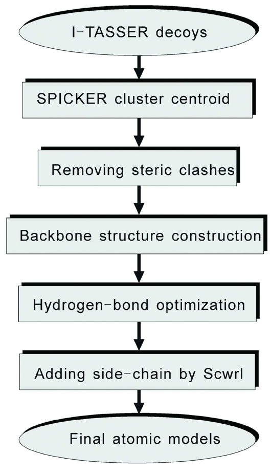
The REMO protocol for constructing full atomic models starting from the I-TASSER cluster centroids.

An on-line server as well as the source code and the executable programs of the REMO algorithm are freely available for academic users at our website: http://zhang.bioinformatics.ku.edu/REMO.

Removing steric clashes

According to the standard in CASP experiment²³, a steric clash is defined as a pair of Cα atoms whose distance is less than 3.6 Å. To remove the steric clashes in the cluster centroids, REMO scans the protein chain and move around each of the Cα atoms that clash with other residues. The direction and magnitude of the movement for ith Cα atom in clash is determined by

$${\stackrel{\rightharpoonup }{v}}_{i,\text{clash}}=c\sum _{j,j\ne i}^L\frac{r_{ij}-r_{\text{c}}}{r_{ij}}\cdot {\stackrel{\rightharpoonup }{r}}_{ij},\forall r_{ij}<r_{\text{c}}$$ (1)

where c is a pre-defined parameter to control the distance of movement; L is the number of residues in the protein chain; r⃑_ij is the vector from the ith to the jth Cα atoms and r_ij is their distance. r_c equals to 3.6 Å in general, but for the residues connected with cis-proline, r_c is set to 2.9 Å. In this way, the two Cα atoms involved in a clash will be directly moved away along the opposite direction.

The purpose of the movement as defined in Eq. (1) is to reduce the clashes of ith Cα with other residues, which, however, may induce new clashes with other groups in the protein chain. To speed up the convergence, we only accept the movements which lead the total “clash energy” E_clash decreasing, i.e.

$$E_{\text{clash}}=|\sum _{i=1}^L{\stackrel{\rightharpoonup }{v}}_{i,\text{clash}}|$$ (2)

The clash removing procedure is iterated by a number of times with a gradually decreasing value of c. Although the clash relaxation uses a steepest-descent minimization procedure which may have danger to trap in local minimum, it actually works surprisingly well and the clashes can be completely removed within 100 iterations which cost only several seconds of the CPU time. The trick here is to carefully tune the parameter of c so that the clashes can be removed quickly but the RMSD between the structures before and after the clash-removal maintains minimum. In our case, by trial and error, we found it works the best when c changes with the number of iterations n in the format of

$$c=\{\begin{array}{ll}0.9u,\hfill & n<32\hfill \\ {(u+0.19)}^2,\hfill & 32\le n<62\hfill \\ 0.79e^{-(u+1)},\hfill & 62\le n<82\hfill \\ 5u^2,\hfill & 82\le n<100\hfill \end{array}$$ (3)

where u=0.7(1−0.01n). In our test, when starting from seriously clashed structures, e.g. the cluster centroid, the RMSD aroused in the clash-removing procedure is less than 1.9 Å; for those with regular local structures, e.g. the close-D, it is almost always less than 0.9 Å. We also attempted to remove the steric clashes by Monte Carlo (MC) simulations. But the MC procedure is less efficient than the presented method in the consideration of the CPU time cost and the number of remaining clashes; this is probably because the Cα clash-removal is essentially a local minimization problem in our formula.

The same idea is also used to eliminate Cα breaks along the initial model. When the distance of a pair of neighboring Cα atoms is larger than 4.1Å, the involved Cα atoms will be moved towards their midpoint.

Backbone isomer library

Starting from the Cα traces with clashes removed, we will build up the backbone heavy atoms by scanning a backbone isomer library collected from the solved high-resolution structures in the PDB library. To construct the isomer library, following filter is used to select a pool of the protein chains: The number of residues in each chain is between 40 and 500; the pair-wise sequence identity between any two chains is lower than 90%; only X-ray structures with a resolution better than 1.6Å are used. Finally, 2,561 protein chains are selected, and 528,798 fragments with four consecutive residues are collected from these protein chains.

We use 6 indices to record the feature of the fragments in our fragment library: (1) residue type of the second residue (labeled as ith residue); (2) secondary structure type of the ith residue (i.e. alpha-helix, beta-strand, coil as defined by Stride²⁴); (3) dihedral angle of the four consecutive Cα atoms which are split into 40 bins in [-180°, 180°]; (4-6) Cα distance of r_i-1,i+1, r_i,i+2, and r_i-1,i+2, where r_i-1,i+1 and r_i,i+2 are split into 10 bins in [4.8Å, 7.3Å] and r_i-1,i+2 into 25 bins in [4.3Å, 10.8Å]. Finally, a 6-dimensinal grid system with 6,000,000 (20*3*40*10*10*25) grid sites is set up and each grid site corresponds to a given 4-residue Cα frame. The positions of the backbone heavy atoms C, N in the second peptide plane are specified in an internal Cartesian coordinates system of (X′, Y′, Z′) (Figure 2):

Figure 2.

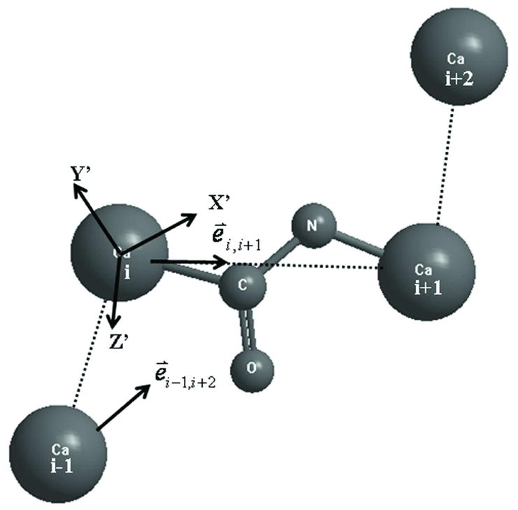
The schematic diagram of internal coordinates system in the backbone isomer library.

$$\{\begin{array}{c}\stackrel{\rightharpoonup }{\text{X}}\text{'}={\stackrel{\rightharpoonup }{e}}_{i-1,i+2}+{\stackrel{\rightharpoonup }{e}}_{i,i+1}\\ \stackrel{\rightharpoonup }{\text{Y}}\text{'}={\stackrel{\rightharpoonup }{e}}_{i-1,i+2}-{\stackrel{\rightharpoonup }{e}}_{i,i+1}\\ \stackrel{\rightharpoonup }{\text{Z}}\text{'}=\stackrel{\rightharpoonup }{\text{X}}\text{'}\times \stackrel{\rightharpoonup }{\text{Y}}\text{'}\end{array}$$ (4)

where e⃑_i−1,i+2 and e⃑_i,i+1 are unit vectors from the (i-1)th to the (i+2)th Cα atom and ith to the (i+1)th Cα atom, respectively.

Because of the regularity of protein local structures, the backbone fragments are highly unevenly distributed in the 6-dimensional grid system, i.e. some grids have multiple redundant fragments and some grids may be empty. To reduce the library size and speed up the backbone construction, we further cluster the backbone conformations of C and N in each grid site based on the pair-wise RMSD of C and N atoms. The RMSD cutoff is selected so that the maximum number of backbone isomers on each grid site is not more than 10. This results in very tight RMSD cutoffs of the isomer clusters. Actually, the maximum RMSD cutoff is <0.05 Å which indicates that all the backbone isomers in the cluster are very close. For each cluster, the cluster centroid is used to represent the backbone isomer. Because of the convergence of the clustered isomers, this choice of cluster centroid does not lead obvious atom clashes. At each grid site, the backbone isomers are deposited in the order of cluster size. Overall, 68,206 non-redundant backbone isomers, which include 19,763 single isomers and 48,443 multiple isomers belonging to 13,150 grid sites, are deposited in our backbone isomer library. Here, our isomer library only records the conformation of Cα, C, and N atoms while the coordinates of O and H are rebuilt based on the conformation of Cα, C, and N atoms using the standard CHARMM22 parameters²⁵.

Predicting hydrogen-bonding network

The hydrogen-bonding network, i.e. a list of hydrogen-bonding donor-acceptor atom pairs, is constructed based on the predicted secondary structure distribution and the global structure of the reduced model. The procedure includes two steps.

In the first step, we generate the secondary structure assignment based on PSI-PRED prediction²⁶ and an initial full atomic model. To construct the initial full atomic model, we thread each of the 4-residue fragments of the reduced model (from the N- to the C-terminal) through the backbone isomer library and pick up the Cα frame which has the lowest RMSD of Cα atoms matching the structure of the reduced model. The first backbone isomer in the matched grid site is used to decide the C and N positions in the second peptide plane of the 4-residue fragment; and then the O and H atoms in this peptide plane are added using the bond length and bond angle from CHARMM22 force field²⁵. If the matched grid site in the backbone isomer library is empty, the isomer closest to the matched grid site will be used. After the construction of the initial full atomic model, a structure-based secondary structure assignment is obtained by running Stride²⁴. The final secondary structure assignment is determined by the consensus of the structure-based secondary structure assignment and a sequence-based secondary structure prediction from PSI-PRED²⁶, i.e. for the regions where the two secondary structure assignments are consistent, the final secondary structure are the same; for the region where the secondary structure assignments are inconsistent, the final secondary structure will be taken from the structure-based assignment for the targets that are classified as “easy” targets in threading^19,27 or from the sequence-based secondary structure predictions otherwise. Finally, a smoothening process is performed to remove the islanded secondary structures which have isolated secondary structure status different from neighboring residues. In detail, if the two neighboring residues in both sides of the ith residue have an identical secondary structure which is different to that of the ith residue, the ith residue will be re-assigned a secondary structure same as its neighbors; while the two residues in both sides of the ith residue have non-identical secondary structures and are also different to that of the ith residue, the ith residue will be re-assigned as coil.

In the second step, following the secondary structure assignment, the detailed hydrogen-bonding network is constructed using the rule as outlined in Figure 3. For the residues in alpha helix, the hydrogen-bonding network is regular and the donor (N) in the (i+4)th residue is always hydrogen-bonded with the acceptor (O) in the ith residue (Fig. 3A).

Figure 3.

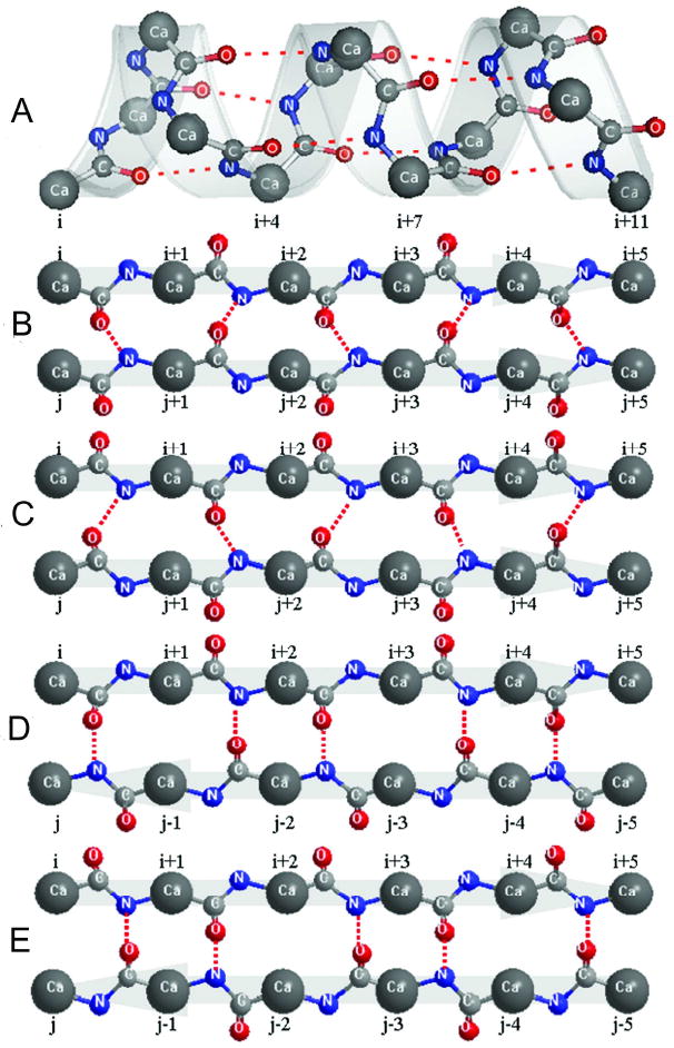
Illustrations of the hydrogen-bonding network in alpha-helix and beta-sheet secondary structures. (A) Hydrogen-bonding network in alpha-helix; (B and C) possible hydrogen-bonding networks in the same parallel beta-sheet; (D and E) possible hydrogen-bonding networks in the same anti-parallel beta-sheet. Dotted lines denote the hydrogen bonds.

To define the hydrogen bond network in beta-sheet, we first decide which strands will form parallel- or anti-parallel beta sheets. For a give pair of strands, we calculate the maximum number of continuous Cα pairs (N_pair) along two strands (including both parallel and anti-parallel directions) which has a spatial distance below L_cut. If N_pair ≥3, the pair of strands are considered as forming a beta-sheet. The value of L_cut depends on whether the considered beta-sheet is parallel or anti-parallel. According to the PDB statistics shown in Figure 4A, we choose L_cut=6.8 Å for parallel and 6.1 Å for anti-parallel beta sheets.

Figure 4.

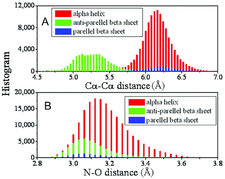
Histogram of distances between atoms in two hydrogen-bonded residues. (A) Cα-Cα distance; (B) the distance of the donor (N) and the acceptor (O) atoms. Different colors indicate the data from different secondary structures.

For a given pair of beta strands, there are always two possible ways to form HB network. For parallel beta sheet with a residue pair list of [(Cα_i, Cα_j), (Cα_i+1, Cα_j+1), (Cα_i+2, Cα_j+2), …], both HB networks of [(O_i, N_j+1), (N_i+2, O_j+1), (O_i+2, N_j+3), …] (Fig. 3B) and [(N_i+1, O_j), (O_i+1, N_j+2), (N_i+3, O_j+2), …] (Fig. 3C) are possible. Similarly, for anti-parallel beta sheet with a residue pair list of [(Cα_i, Cα_j), (Cα_i+1, Cα_j-1), (Cα_i+2, Cα_j-2), …], both HB networks of [(O_i, N_j), (N_i+2, O_j-2), (O_i+2, N_j-2), …] (Fig. 3D) and [(N_i+1, O_j-1), (O_i+1, N_j-1), (N_i+3, O_j-3), …] (Fig. 3E) are possible. For selecting the appropriate network, we calculate the average distance of all donor (N)-acceptor (O) pairs in both possible HB networks based on the initial full atomic model built as above, and then select the one which has the minimum deviation from the experimental distance of 3.2 Å (see Figure 4B). After all the hydrogen bonds in the secondary structure are determined, an expected hydrogen bond list with all donor-acceptor pairs along the chain is generated.

Hydrogen-bonding enriched backbone structure refinement

With the purpose of having more hydrogen-bonds in the structural models that are consistent with the expected backbone hydrogen-bonding list, we optimize the backbone hydrogen-bonding network in two steps.

Step1, maximizing HB-network with Cα fixed

We first calculate hydrogen-bonds in the initial full atomic model. For the regions where the expected hydrogen bonds are satisfied, all the backbone atoms are frozen; for other regions, we sample the conformation of the peptide plane by randomly adopting the conformation from the backbone isomers in the library which belong to the same Cα-frame (i.e. the same grid site in the 6-dimensional backbone isomer system) or near the matched grid site, trying to maximize the number of hydrogen-bonds. It's worthy to emphasize that this isomer swap do not change the position of any Cα atoms. If a new conformation of the peptide plane satisfies the expected hydrogen-bonding list, the new conformation will be accepted and all the backbone atoms in this peptide plane will be fixed.

Step2, Monte Carlo optimization with Cα flexible

The energy of our Monte Carlo simulation is defined as

$$E_{\text{opt}}=w_1{E}_{\text{res}}+w_2{E}_{\text{clash}}+w_3{E}_{\text{Hbond}}+w_4{E}_{\text{RMSD}}$$ (5)

E_res counts for the spatial restraints collected from multiple threading templates²⁷ which include Cα and side-chain contacts, and Cα distance map, i.e.

$$E_{\text{res}}=\sum _{i>j}\Theta (r_{ij}-6)+\sum _{k>l}\Theta (R_{kl}-d_0)-\sum _{m>n}\frac{1}{\Delta (|r_{mn}-r_{mn}^0|)}$$ (6)

where r_ij is the distance of Cα atoms in the model and the sum of i and j goes through the residue pairs with Cα atoms predicted in contact; R_kl is the distance of side-chain centers in the model and k and l goes through residue pairs with side-chains predicted in contact; $r_{mn}(r_{mn}^0)$ is the actual (predicted) distances between Cα atoms; d₀ is an amino-acid specific distance cutoff for side-chain contacts²⁰; Θ(x) equals -1 if x < 0, otherwise equals 0; Δ(x) equals 1 if x < 1, otherwise equals x. This term is the same as that used in the I-TASSER simulations.

E_clash in Eq. (5) is the summation of the steric clash energy for each residue as defined in Eq. (2). E_Hbond counts for the hydrogen bond energy which equals to the sum of the number of total backbone hydrogen-bonds plus the number of hydrogen-bonds which satisfy the expected backbone HB-list. This term encourages all the hydrogen-bonds with the expected hydrogen-bonds double counted. E_RMSD equals to the Cα RMSD between the current conformation and the initial structure. The purpose of this term is to keep the global topology of the model near the initial structure. The weight factors of w₁, w₂, w₃ and w₄ are tuned by hand and taken as L^-0.5, 5.0, -1.0 and 10.0, respectively, where L is the number of residues in protein chain.

The movement of our simulations depends on the current conformations. For the ith residue, the expected motion of the Cα atom is defined as (see Figure 5)

Figure 5.

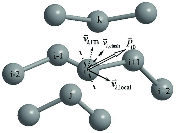
The schematic illustration for determining the expected movement P⃑_i0 of the ith Cα atom. The dashed, dotted, and solid vectors show the contributions from steric clash (from j), hydrogen-bonding (with k), and irregular local structure (from i-1) to the expected movement, respectively. The dashed-dotted line is vertical to P⃑_i0 and random movements always point to the same side of P⃑_i0.

$${\stackrel{\rightharpoonup }{P}}_{i0}={\stackrel{\rightharpoonup }{v}}_{i,\text{clash}}+{\stackrel{\rightharpoonup }{v}}_{i,\text{HB}}+{\stackrel{\rightharpoonup }{v}}_{i,\text{local}}$$ (7)

where v⃑_{i, clash} is defined in Eq. (2) in the direction to eliminate steric clashes. v⃑_i,HB denotes the expected motion for the Cα to follow the expect hydrogen-bonding, i.e.

$${\stackrel{\rightharpoonup }{v}}_{i,\text{HB}}=\sum _j^{N_{HB}^i}\frac{r_{ij}-r_0}{r_{ij}}{\stackrel{\rightharpoonup }{r}}_{i,j},\forall |r_{ij}-r_0|>{\sigma }_0$$ (8)

where r₀ and σ₀ are the average Cα-Cα distance and the statistical deviation for hydrogen-bonds at each type of secondary structure (as listed Table 1). $N_{HB}^i$ is the number of expected hydrogen-bonds whose donor or acceptor is from the ith residue. The form of v⃑)_i,local, which counts for the local Cα-distances of residues i with i±1 and i±2, has a similar form as Eq. (8). For i and i±1, r₀=3.8 Å and σ₀ = 0.2 Å; for i and i±2, the distance parameters are listed in the right two columns in Table 1.

Table 1.

Parameters used in Monte Carlo simulations to refine backbone hydrogen bonding network. Equilibrium Cα distances (r₀) and the deviation (σ₀) are used in guiding the Cα movements as described in Eqs. (7) and (8). “HB” indicates that for the hydrogen-bonded atoms and “Local” for the distance of i to i±2th residues.

Secondary structures	HB		Local
	r0 (Å)	σ0 (Å)	r0 (Å)	σ0 (Å)
Alpha-helix	6.15	0.53	5.55	0.55
Parallel beta-sheet	6.20	0.50	6.60	0.80
Anti-parallel beta-sheet	5.20	0.60	6.60	0.80

The vector of real movement of the Cα atoms in our simulation is defined as

$${\stackrel{\rightharpoonup }{P}}_i=\text{ran}{d}_1\ast P_{i0,x}\ast \stackrel{\rightharpoonup }{x}+\text{ran}{d}_2\ast P_{i0,y}\ast \stackrel{\rightharpoonup }{y}+\text{ran}{d}_3\ast P_{i0,z}\ast \stackrel{\rightharpoonup }{z}$$ (9)

where rand_1,2,3 are random numbers between 0 and 1, (P_i0,x, P_i0,yP_i0,z) is the projection of P⃑_i0 in absolute coordinates system with x⃑, y⃑, z⃑ as unit vectors. This movement will be always oriented towards the same side of the expected motion vector P⃑_i0.

Following each movement of the Cα atoms, the conformation of C, N and O in the same residue of the Cα atoms will be translated by a displacement of P⃑_i. If any of the bond length or bond angles in the new conformation has a violation of 10% from the CHARMM22 parameters, the peptide atoms will be reconstructed from our backbone isomer library following the procedure in Step 1.

The trail movement will be accepted or rejected based on the Metropolis criterion²⁸ with the energy function defined as Eq. (5). It is worth to note that our simulation is not identical to the conventional Metropolis Monte Carlo simulation because our movements are anisotropic with bias to the direction to reduce steric clash, enhance hydrogen-bonding and regularize local structure. This may have the danger in violating the ergodicity which is important in global minimization search. In our case of structure refinement which is essentially a local minimization, we find that it converges faster than the isotropic movements.

After a set of 100L attempted movements in Cα relocations, we readjust the full atomic conformation with Cα fixed as described in Step 1. The iteration of Step 1 and Step 2 will be repeated for a number of times till the E_opt versus the simulation time converged, which normally take the CPU time less than 10 minutes at a 2.6 GHz AMD processor. The final model will be selected based on the highest combined hydrogen-bond score which is defined as the number of backbone hydrogen bonds plus the backbone hydrogen bonds that is in the expected hydrogen bond list.

Evaluation criterions

For the evaluation of global topology of the final models, we use both RMSD and TM-score to relative to the native structure. While RMSD can give an explicit concept of modeling errors, a local error (e.g., tail misorientation) can cause a large RMSD value although the global topology is correct. TM-score is defined as⁷

$$\text{TM}-\text{score}=\frac{1}{L}\sum _{i=1}^L\frac{1}{1+{(d_i/d_0)}^2}$$ (10)

where d_i is the distance of the ith Cα pair between model and the native after superposition, and $d_0=1.24\sqrt[3]{L-15}-1.8$. Since TM-score weights small distances stronger than the larger distances, it is more sensitive to the global topology than RMSD. According to Zhang and Skolnick⁷, TM-score=1 indicates two identical structures, TM-score<0.17 indicates random structure pairs, and TM-score>0.5 indicates two structures have approximately the same fold.

To evaluate the secondary structure, the hydrogen-bonding score (HB-score) is defined

$$\text{HB}-\text{score}=\frac{\text{number of consensus hydrogen bonds in model and native}}{\text{number of hydrogen bonds in the native structure}}$$ (11)

The hydrogen bonds in full atomic structures are defined by Hbplus ¹².

Results

Dataset and reduced models

A non-redundant set of 230 proteins are collected from the PDB library which have a length ranging from 80 to 300 residues. The sequence identity of any two proteins in this set is lower than 30% and all are solved by X-ray crystallography with a resolution better than 1.6 Å. There are overall 39 alpha-, 44 beta- and 147 alpha/beta-proteins in the test set.

The reduced models are generated by the I-TASSER simulations⁵ with threading templates identified by MUSTER¹⁹ where all homologous templates with sequence identity to the target higher than 30% are excluded. Forty replicas have been used in the I-TASSER simulation and the trajectories in 8 low-temperature replicas are clustered by the SPICKER program⁸. The RMSD of the cluster centroid of the first clusters ranges from 1.2 Å to 25 Å, which covers a resolution region typically seen in protein structure predictions^1,11.

Removal of steric clashes

Because the structure of cluster centroids in SPICKER is built by averaging the coordinates of all structure decoys in the same cluster, the substructure of the cluster centroid can be completely distorted. A significant challenge is to construct a full atomic model which has regular substructures and meanwhile retains similar or better topology score as the cluster centroids.

To quantitatively count the distortion of the substructures in the Cα traces, the number of steric clashes (N_clash) is calculated. Here, we follow the standard used in the CASP experiment²³ and define a steric clash as a pair of Cα atoms whose distance is less than 3.6 Å. The number of steric clashes in the cluster centroids depends on the diversity of the structure decoys in the clusters which is related with the difficulties of the modeling targets. For easy targets, the simulation trajectories are convergent, the average of similar structures does not result too many distortions; however, for hard targets, the average from diverged trajectories results in lots of clashes. In our benchmark set, which include 143 easy targets and 87 medm/hard targets according to the definition by MUSTER¹⁹, the average number of clashes in the cluster centroids is 119. The number of clashes of individual target ranges from 1 to 395. After the REMO clash-removing procedure, only 15 targets have 2-6 clashes, 44 targets have one clash, and in the remaining targets all clashes are removed (Figures 6A and 6B). For these targets which still have several clashes, most of them are due to the existence of cis-proline in turn, where the standard distance between neighboring Cα atoms is around 2.9Å.

Figure 6.

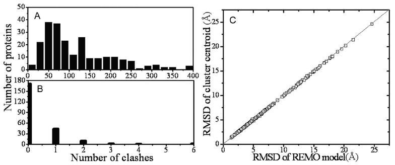
Distribution of the number of clashes and RMSD in the cluster centroids and REMO model. (A) Histogram of steric clashes in the cluster centroids; (B) histogram of steric clashes in the REMO models; (C) RMSD to native of the REMO models versus that of the cluster centroids.

In previous modeling experiments^4,5,20, to avoid steric clashes in the final models, we generated full atomic models based on individual structural decoys, where the topology of the final models usually has worse structural similarity to native than the cluster centroid. In Figure 6C, we compare the RMSD of the REMO models to the native with that of the cluster centroids. Remarkably, although the steric clashes have been completely removed, the clash-removing procedure has no side-effect on the globular topology of the initial structures.

As a comparison, we list in Table 2 the results of the full atomic models generated by other popularly-used programs, including MODELLER¹⁶, NEST¹⁴, PULCHRA¹³, and MAXSPROUT¹⁵. All the full atomic models are constructed from the same set of cluster centroids. For MAXSPROUT, because it can successfully generate full atomic models only for 18 proteins, all of which are easy targets and have fewer steric clashes, we list these proteins separately in the last two rows. For other programs, although they could generate full atomic models, none of them can efficiently remove the steric clashes, which indicates that serious distorted substructures exist in these models.

Table 2.

Comparison of atomic structures built by different programs based on the same initial reduced models. Npro is the number of targets that full atomic model was successfully constructed.

Methods/Structures	Npro	RMSD (Å)	TM-score	HB-score	Nclash
MODELLER	230	7.11	0.637	0.216	36.1
NEST	230	7.11	0.636	0.275	27.0
PULCHRA	230	7.12	0.637	0.338	23.5
REMO	230	7.09	0.639	0.343	0.4
MAXSPROUT	18	2.69	0.825	0.434	6.4
REMO	18	2.68	0.827	0.454	0.2

It may not be entirely fair to compare REMO with other programs based on the cluster centroids because most of these tools have been trained on the well-behaved structures and therefore try to reconstruct atomic models close to the initial coarse-grained models. In the next section, we will compare the REMO models with the models built by other programs based on reduced models with fewer clashes.

Comparison of REMO model with I-TASSER model

Since the conventional software could not completely remove the steric clashes in the structure of cluster centroids, we usually generate full atomic models from individual structure decoys. In CASP6 and CASP7 experiments^18,29, for example, we build atomic models using PULCHRA, and starts from close-D, the structure decoy that is the closest to the cluster centroid. Because the structure of the close-D has much less steric clashes than that in the cluster centroids, most of the software can build full atomic models free of clashes. We selected PULCHRA because it generates models with on average slightly higher TM-score and HB-score than that by using MODELLER or NEST.

In Figure 7, we present the HB-score of the REMO models in comparison with that of the I-TASSER models. For the 230 testing proteins, there are 187 targets where the REMO models have a higher HB-score. The remaining 35 (or 8) targets have models with a lower (or equal) HB-score than that of the I-TASSER models. This results in a 24% of improvement of the total HB-score by REMO over I-TASSER. The HB-score difference between the REMO models and the I-TASSER models varies from -0.104 to 0.284, with the absolute number of difference in correctly reconstructed hydrogen bonds ranging form -15 to 44. If we split the proteins into alpha-, beta-, and alpha/beta-proteins, the HB-score improvements are 28.7%, 18.6%, and 23.1% in these categories (see Table 3), respectively; the HB-score improvement by REMO is most pronounced in helix structures.

Figure 7.

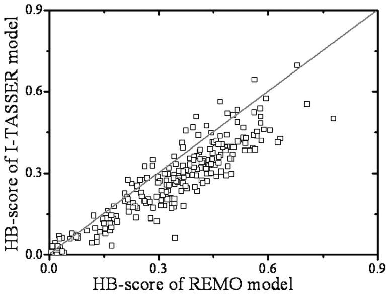
HB-score of the REMO models versus that of the I-TASSER models.

Table 3.

Summary of comparison of the REMO (RE) and the I-TASSER (IT) models.

Protein type	RMSD (Å)		TM-score		HB-score
	IT	RE	IT	RE	IT	RE
Alpha	7.52	7.16	0.606	0.624	0.373	0.480
Beta	8.52	8.08	0.570	0.588	0.177	0.210
Alpha/beta	7.09	6.79	0.642	0.658	0.281	0.346
Total	7.43	7.10	0.622	0.639	0.277	0.343

Because the REMO models are generated by the optimization of the predicted hydrogen-bonding networks, the HB-score improvement is highly correlated with the accuracy of the predicted HB-list. For the 35 cases where the REMO models have a worse HB-score than I-TASSER, the average accuracy of the HB-list is 0.51 and the correctly predicted hydrogen-bonds cover 47.5% of all the backbone hydrogen bonds in the native structures; this is obviously lower than those of other proteins which have an average accuracy of 0.56 for HB-list and the correct hydrogen-bonds covers 54.9% of the native structures. The reason for the low accuracy of HB-list is that for some targets the initial full atomic models built from the cluster centroids after clash removal still have some distorted secondary structures. When combining these models with PSI-PRED predictions, the predicted HB-list can be spoiled in the distorted regions. One solution to the problem is to reconstruct HB-list from the final REMO models and repeat the whole procedure iteratively although it will take a longer CPU time. Nevertheless, more than 80% (187/230) of the targets have the final REMO models with an improved HB-score, which demonstrates that the majority of the hydrogen-bonds have been correctly predicted in the HB-list by the current procedure and the predicted HB network has been efficiently implemented in the atomic models.

As a direct test of the sensitivity of HB-list, we have run REMO without using the PSI-PRED prediction; the HB-score of the REMO models is reduced by 11.4% with the average HB-score decreased from 0.343 to 0.304. Simultaneously, the average RMSD and TM-score of the final model changed slightly, i.e. from 7.096Å (0.6390) to 7.084Å (0.6388).

In Figures 8A and 8B, we present the RMSD and TM-score of the REMO models versus those of the I-TASSER models. For 230 proteins, there are 209 targets where the REMO models have a lower RMSD to the native structures. Most of the visible improvements occur in the large RMSD regions (say RMSD>5Å). But even for the models in the region of 1-5 Å, there are still clearly more points which are above the diagonal line which indicates RMSD improvements (see the Inset of Figure 8A). If considering TM-score, REMO outperforms I-TASSER in 214 cases. The improvements occur in almost all the range of TM-score values (see Figure 8B). This difference in the improvement regions is probably due to the fact that RMSD is not a measure sensitive to topology and many models of high RMSD to the native may still have a similar topology as native when measured by the TM-score.

Figure 8.

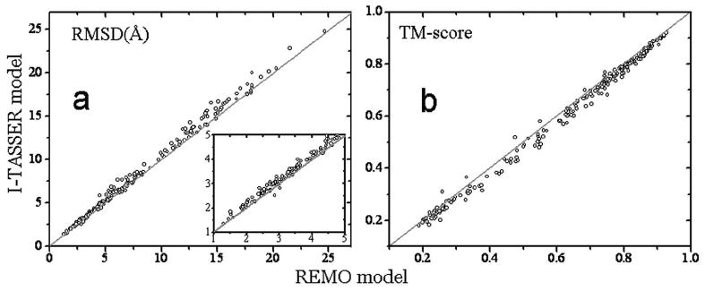
The comparison of RMSD (A) and TM-score (B) between the REMO and the I-TASSER models. The inset in A is a zoom-in of the figure in the region of [1Å, 5Å].

In Figure 9, we present three typical examples of alpha-, beta-, and alpha/beta-proteins by REMO (Right panel); these show clear improvements in both TM-score and secondary structure constructions compared to the I-TASSER models (Left panel).

Figure 9.

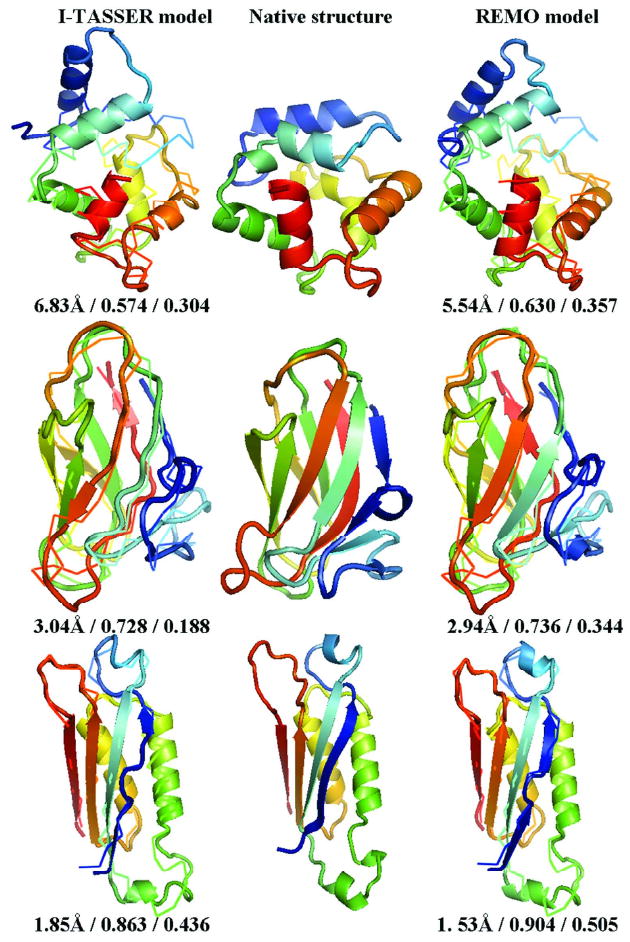
Three illustrative examples of alpha- (PDB id: 2pvb), beta- (1w0n), and alpha/beta- (1nbu) proteins. The cartoons of the native structures are listed in the middle panel. The models in Left and Right panels are built using the I-TASSER protocol and REMO, respectively. Models (in cartoons) are superimposed on the native (in backbones). Blue to red runs from N- to C-terminals. The values under each model indicate RMSD, TM-score and HB-score, respectively.

In Table 3, we summarize the results of the REMO modeling in different secondary structure categories, which are also compared with that by I-TASSER. Among the three types of proteins, the beta-proteins have the largest improvement in the global topology, where RMSD is reduced by 5.2% and TM-score is increased by 3.2%, and the alpha-proteins have the largest HB-score improvement as mentioned above (by 28.7%). Overall, RMSD in REMO models has a reduction of 4.5%, TM-score has an improvement of 2.7% and HB-score is improved by 23.8% for all 230 proteins. Although the REMO model has on average 0.4 Cα steric clashes, which is mainly due to the cis-proline conformations. It is close to that of the PDB structures where the average number of Cα clashes is 0.6 when we check the 230 experiment structures. Here, it is worthy to mention that the refinement induced by REMO cannot change the category of the biological usefulness of the original models³⁰. But for the practical use in optimizing hydrogen-bonding networks and refining atomic details of distorted models, these improvements are still encouraging.

Finally, as a qualitative assessment of the local geometry, we examine the backbone phi/psi dihedral angle distribution of the REMO models. For this propose, we draw the standard Ramachandran plot with data calculated from 7,615 protein chains which are solved by X-ray and with a resolution higher than 2.0 Å (plot not shown). If we divide the phi-psi angle space into 10×10-degree lattices and define a lattice as “physically allowed” when there are at least one native residue appearing on the lattice, 98.8% of residues in the REMO models are physically allowed. This number is similar as that in the I-TASSER models by PULCHRA (98.7%) and the model by MODELLER (99.2%).

Concluding Remarks

We developed a new protocol of REMO to construct atomic protein models from Cα traces by first removing steric clashes and then optimizing the hydrogen-bonding networks with fragments matched from a newly constructed backbone isomer library. The benchmarking test shows significant advantage of REMO in refining both the global topology and the local geometry compared with the current atomic model construction approaches in literatures.

As a blind test, we have used the REMO protocol in the recent CASP8 experiment for refining the reduced models by I-TASSER simulations. Based on the 172 released targets/domains, the average TM-score and GDT-score of the “Zhang-Server” models are higher with a significant margin than that of other groups in the server section (see http://zhang.bioinformatics.ku.edu/casp8). Especially, the average HB-score of the “Zhang-Server”, which partially reflects the quality of local structures, is also higher than all other groups except for SAM-08-server, while in CASP7 the HB-score of the I-TASSER models in our lab is lower than most of other groups^11,31. These data demonstrate significant progress in reconstructing and refining atomic models using the REMO protocol.

There are two factors which have key contributions to the efficiency of the REMO algorithm. First, the REMO procedure can efficiently remove the steric clashes in seriously distorted cluster centroids and quickly generate models which have reasonable bond length and bond angle. Because the cluster centroids have on average better RMSD and TM-score than individual decoys, this procedure is the major contribution to the improvement of the global topology of final atomic models. Second, the hydrogen-bonding network has been accurately predicted and constructed from the consensus of PSI-PRED predicted secondary structure distribution and the initial atomic structure directly build from the SPICKER centroids. Our Monte Carlo simulation procedure optimizes the hydrogen-bonding network through a secondary-structure specific backbone isomer library, which significantly improves the local geometry and hydrogen-bonding network of the final models.

Although the REMO method has been benchmarked here on the I-TASSER decoys, it should be able to use in constructing full atomic models from distorted Cα traces generated by other approaches. For example, in the 3D-SHOTGUN based meta-server approaches³², hybrid structure models are constructed by cutting-and-pasting structure fragments from multiple templates as identified by a number of threading programs. Although the global topology score of the 3D-SHOTGUN models is higher than the individual threading templates, there are serious steric clashes in the backbone of the hybrid models. The significant ability of REMO in removing the steric clashes and refining hydrogen-bonding networks should be a useful solution to these problems.

Abbreviation

Cα

alpha carbon

HB

Hydrogen Bond

RMSD

root mean square deviation

References

- 1.Zhang Y. Progress and challenges in protein structure prediction. Current opinion in structural biology. 2008;18(3):342–348. doi: 10.1016/j.sbi.2008.02.004. [DOI] [PMC free article] [PubMed] [Google Scholar]
- 2.Oldziej S, Czaplewski C, Liwo A, Chinchio M, Nanias M, Vila JA, Khalili M, Arnautova YA, Jagielska A, Makowski M, Schafroth HD, Kazmierkiewicz R, Ripoll DR, Pillardy J, Saunders JA, Kang YK, Gibson KD, Scheraga HA. Physics-based protein-structure prediction using a hierarchical protocol based on the UNRES force field: assessment in two blind tests. Proceedings of the National Academy of Sciences of the United States of America. 2005;102(21):7547–7552. doi: 10.1073/pnas.0502655102. [DOI] [PMC free article] [PubMed] [Google Scholar]
- 3.Simons KT, Ruczinski I, Kooperberg C, Fox BA, Bystroff C, Baker D. Improved recognition of native-like protein structures using a combination of sequence-dependent and sequence-dependent and sequence-independent features of proteins. Proteins. 1999;34:82–95. doi: 10.1002/(sici)1097-0134(19990101)34:1<82::aid-prot7>3.0.co;2-a. [DOI] [PubMed] [Google Scholar]
- 4.Zhang Y, Skolnick J. Automated structure prediction of weakly homologous proteins on a genomic scale. Proceedings of the National Academy of Sciences of the United States of America. 2004;101:7594–7599. doi: 10.1073/pnas.0305695101. [DOI] [PMC free article] [PubMed] [Google Scholar]
- 5.Wu S, Skolnick J, Zhang Y. Ab initio modeling of small proteins by iterative TASSER simulations. BMC biology. 2007;5:17. doi: 10.1186/1741-7007-5-17. [DOI] [PMC free article] [PubMed] [Google Scholar]
- 6.Kabsch W. A solution for the best rotation to relate two sets of vectors. Acta Cryst. 1976;A32:922–923. [Google Scholar]
- 7.Zhang Y, Skolnick J. Scoring function for automated assessment of protein structure template quality. Proteins. 2004;57:702–710. doi: 10.1002/prot.20264. [DOI] [PubMed] [Google Scholar]
- 8.Zhang Y, Skolnick J. SPICKER: A clustering approach to identify near-native protein folds. Journal of computational chemistry. 2004;25(6):865–871. doi: 10.1002/jcc.20011. [DOI] [PubMed] [Google Scholar]
- 9.Simons KT, Kooperberg C, Huang E, Baker D. Assembly of protein tertiary structures from fragments with similar local sequences using simulated annealing and Bayesian scoring functions. Journal of molecular biology. 1997;268(1):209–225. doi: 10.1006/jmbi.1997.0959. [DOI] [PubMed] [Google Scholar]
- 10.Shortle D, Simons KT, Baker D. Clustering of low-energy conformations near the native structures of smalle proteins. Proc Natl Acad Sci USA. 1998;95:11158–11162. doi: 10.1073/pnas.95.19.11158. [DOI] [PMC free article] [PubMed] [Google Scholar]
- 11.Kopp J, Bordoli L, Battey JN, Kiefer F, Schwede T. Assessment of CASP7 predictions for template-based modeling targets. Proteins. 2007;69(S8):38–56. doi: 10.1002/prot.21753. [DOI] [PubMed] [Google Scholar]
- 12.McDonald IK, Thornton JM. Satisfying hydrogen bonding potential in proteins. Journal of molecular biology. 1994;238(5):777–793. doi: 10.1006/jmbi.1994.1334. [DOI] [PubMed] [Google Scholar]
- 13.Rotkiewicz P, Skolnick J. Fast procedure for reconstruction of full-atom protein models from reduced representations. Journal of computational chemistry. 2008;29(9):1460–1465. doi: 10.1002/jcc.20906. [DOI] [PMC free article] [PubMed] [Google Scholar]
- 14.Petrey D, Xiang Z, Tang CL, Xie L, Gimpelev M, Mitros T, Soto CS, Goldsmith-Fischman S, Kernytsky A, Schlessinger A, Koh IY, Alexov E, Honig B. Using multiple structure alignments, fast model building, and energetic analysis in fold recognition and homology modeling. Proteins. 2003;53 6:430–435. doi: 10.1002/prot.10550. [DOI] [PubMed] [Google Scholar]
- 15.Holm L, Sander C. Database algorithm for generating protein backbone and side-chain co-ordinates from a C alpha trace application to model building and detection of co-ordinate errors. Journal of molecular biology. 1991;218(1):183–194. doi: 10.1016/0022-2836(91)90883-8. [DOI] [PubMed] [Google Scholar]
- 16.Sali A, Blundell TL. Comparative protein modelling by satisfaction of spatial restraints. Journal of molecular biology. 1993;234(3):779–815. doi: 10.1006/jmbi.1993.1626. [DOI] [PubMed] [Google Scholar]
- 17.Zhang Y, Skolnick J. Tertiary structure predictions on a comprehensive benchmark of medium to large size proteins. Biophysical journal. 2004;87:2647–2655. doi: 10.1529/biophysj.104.045385. [DOI] [PMC free article] [PubMed] [Google Scholar]
- 18.Zhang Y. Template-based modeling and free modeling by I-TASSER in CASP7. Proteins. 2007;69(S8):108–117. doi: 10.1002/prot.21702. [DOI] [PubMed] [Google Scholar]
- 19.Wu ST, Zhang Y. MUSTER: Improving Protein Sequence Profile-Profile Alignments by Using Multiple Sources of Structure Information. Proteins. 2008 doi: 10.1002/prot.21945. [DOI] [PMC free article] [PubMed] [Google Scholar]
- 20.Zhang Y, Kolinski A, Skolnick J. TOUCHSTONE II: A new approach to ab initio protein structure prediction. Biophysical journal. 2003;85:1145–1164. doi: 10.1016/S0006-3495(03)74551-2. [DOI] [PMC free article] [PubMed] [Google Scholar]
- 21.Zhang Y, Kihara D, Skolnick J. Local energy landscape flattening: Parallel hyperbolic Monte Carlo sampling of protein folding. Proteins. 2002;48:192–201. doi: 10.1002/prot.10141. [DOI] [PubMed] [Google Scholar]
- 22.Canutescu AA, Shelenkov AA, Dunbrack RL., Jr A graph-theory algorithm for rapid protein side-chain prediction. Protein Sci. 2003;12(9):2001–2014. doi: 10.1110/ps.03154503. [DOI] [PMC free article] [PubMed] [Google Scholar]
- 23.Tress M, Ezkurdia I, Grana O, Lopez G, Valencia A. Assessment of predictions submitted for the CASP6 comparative modeling category. Proteins. 2005;61 7:27–45. doi: 10.1002/prot.20720. [DOI] [PubMed] [Google Scholar]
- 24.Frishman D, Argos P. Knowledge-based protein secondary structure assignment. Proteins. 1995;23(4):566–579. doi: 10.1002/prot.340230412. [DOI] [PubMed] [Google Scholar]
- 25.MacKerell AD, Bashford D, Bellott M, Dunbrack RL, Evanseck JD, Field MJ, Fischer S, Gao J, Guo H, Ha S, Joseph-McCarthy D, Kuchnir L, Kuczera K, Lau FTK, Mattos C, Michnick S, Ngo T, Nguyen DT, Prodhom B, Reiher WE, Roux B, Schlenkrich M, Smith JC, Stote R, Straub J, Watanabe M, Wiorkiewicz-Kuczera J, Yin D, Karplus M. All-Atom Empirical Potential for Molecular Modeling and Dynamics Studies of Proteins. J Phys Chem B. 1998;102(18):3586–3616. doi: 10.1021/jp973084f. [DOI] [PubMed] [Google Scholar]
- 26.Jones DT. Protein secondary structure prediction based on position-specific scoring matrices. J Mol Biol. 1999;292:195–202. doi: 10.1006/jmbi.1999.3091. [DOI] [PubMed] [Google Scholar]
- 27.Wu S, Zhang Y. LOMETS: a local meta-threading-server for protein structure prediction. Nucleic acids research. 2007;35(10):3375–3382. doi: 10.1093/nar/gkm251. [DOI] [PMC free article] [PubMed] [Google Scholar]
- 28.Metropolis N, Rosenbluth AW, Rosenbluth MN, Teller AH, Teller E. Equation of state calculations by fast computing machines. J Chem Phys. 1953;21:1087–1092. [Google Scholar]
- 29.Zhang Y, Arakaki A, Skolnick J. TASSER: An automated method for the prediction of protein tertiary structures in CASP6. Proteins. 2005;61 7:91–98. doi: 10.1002/prot.20724. [DOI] [PubMed] [Google Scholar]
- 30.Zhang Y. Protein structure prediction: Is it useful? Corr Opin Struct Biol. 2009 doi: 10.1016/j.sbi.2009.02.005. In press. [DOI] [PMC free article] [PubMed] [Google Scholar]
- 31.Battey JN, Kopp J, Bordoli L, Read RJ, Clarke ND, Schwede T. Automated server predictions in CASP7. Proteins. 2007;69(S8):68–82. doi: 10.1002/prot.21761. [DOI] [PubMed] [Google Scholar]
- 32.Fischer D. 3D-SHOTGUN: a novel, cooperative, fold-recognition meta-predictor. Proteins. 2003;51(3):434–441. doi: 10.1002/prot.10357. [DOI] [PubMed] [Google Scholar]