Classification of hematologic malignancies using texton signatures

Abstract

We describe a decision support system to distinguish among hematology cases directly from microscopic specimens. The system uses an image database containing digitized specimens from normal and four different hematologic malignancies. Initially, the nuclei and cytoplasmic components of the specimens are segmented using a robust color gradient vector flow active contour model. Using a few cell images from each class, the basic texture elements (textons) for the nuclei and cytoplasm are learned, and the cells are represented through texton histograms. We propose to use support vector machines on the texton histogram based cell representation and achieve major improvement over the commonly used classification methods in texture research. Experiments with 3,691 cell images from 105 patients which originated from four different hospitals indicate more than 84% classification performance for individual cells and 89% for case based classification for the five class problem.

1 Introduction

Over the past few years there has been increased interest and efforts applied to utilizing content-based image retrieval in medical applications [18, 24, 25, 28, 29, 41]. Individual strategies and approaches differ according to the degree of generality (general purpose versus domain specific), the level of feature abstraction (primitive features versus logical features), overall dissimilarity measure used in retrieval ranking, database indexing procedure, level of user intervention (with or without relevance feedback), and by the methods used to evaluate their performance. In this paper, we present a decision system utilizing texture based representation and support vector machine (SVM) optimization to classify hematologic malignancies.

The use of texture analysis for performing automated classification of disease based on features extracted from radiological imaging studies has been reported in the medical literature repeatedly. It has been successfully applied in breast cancer [32, 33, 42], liver cancer [23] and obstructive lung disease [2].

Recently there have been a number of investigators who have begun to explore the feasibility of utilizing texture features in the classification of pathology at the microscopic level. The success of the methods vary with the domain of the problem, and the choice of representation and optimization techniques. We also note that the testing methodology that is applied during the experiments and the size of the datasets have very important role in the observed results, and some test methodologies and small datasets can trigger biased results.

In [37], frequency domain features are used to classify among subclasses of normal and abnormal cervical cell images using a database containing 110 cells from both normal and abnormal groups. Using the spectra of cell images, 27 texture features are extracted with gray level difference method and together with 22 frequency components, resulted in 92% correct classification among subclasses. In [46], statistical geometric features, which are computed from several binary thresholded versions of texture images are used to classify among normal and abnormal cervical cells. The method gave 93% correct classification rate on a database containing 117 cervical cells using only 9 statistical features.

A discrimination scheme among the main subsets of lung carcinomas was reported in [40] by chromatin texture feature analysis using a test set comprised of 195 specimens. Texture features describing the granularity and the compactness of the nuclear chromatin were extracted for calculation of classification rules, which allowed the discrimination of different tumor groups. Although the classification failed to distinguish among some subtypes of tumor groups, around 90% classification accuracy was achieved for small-cell and non-small-cell lung carcinoma using the four dimensional texture features combined with simple decision rules.

In [34], adaptive texture features were described utilizing the class distances and differences of gray level cooccurrence matrices of texture images. In [35], the adaptive texture features were used for classifying the nuclei of cells in ovarian cancer. In this study a clear relation between nuclear DNA content, area, first-order statistics, and texture is observed. The approach discriminated the two classes of cancer with a correct classification rate of 70% on a test set of 134 cases.

A decision support system to discriminate among three types of lymphoproliferatie disorders and normal blood cells was presented in [5]. Cells were represented with their nuclear shape, texture and area, where shape was characterized through similarity invariant Fourier descriptors and multiresolution simultaneous autoregressive model was utilized for texture description. The experiments conducted on a database consisting of 261 specimens using tenfold cross validation were resulted with 80% correct classification rate. Notice that in all the methods described, the results were acquired using small datasets and without obeying the separation of cells among training–testing sets based on patient. We present a detailed discussion about the testing methodologies and their effects on the results in Sect. 5.

As new treatments emerge, each targeting specific clinical profiles, it becomes increasingly important to distinguish among subclasses of pathologies. In modern diagnostic pathology, sophisticated analyses are often needed to support a differential diagnosis, but these supporting tests are not typically employed unless morphological assessment of a specimen first leads one to classify the case as suspicious. In many cases, the differential diagnosis can only be rendered after immunophenotyping and/or molecular or cytogenetic study of the cells involved. Immunophenotyping is the process commonly used to analyze and sort lymphocytes into subsets based on their antigens using flow cytometry. For the purposes of our experiments the immunophenotype provide independent confirmation of the diagnosis for all cases. The additional studies are expensive, time consuming, and usually require fresh tissue which may not be readily available. Since it is impractical to immunophenotype every sample that is flagged by a complete blood count (CBC) device, passing the specimen through a reliable image-based screening system could potentially reduce cost and patient morbidity.

We designed a texture based solution which distinguishes between normal cells and four different hematologic malignancies. We discriminate among lymphoproliferatie disorders, chronic lymphocytic leukemia (CLL), mantle cell lymphoma (MCL), follicular center cell lymphoma (FCC), which can be confused with one another during routine microscopic evaluation. Two acute leukemias, acute myelocytic leukemia (AML) and acute lymphocytic leukemia (ALL), could only be classified in relation to the lymphoproliferatie disorders and normal cells as a single unit labeled as acute leukemia. It is shown in [36] that there is no statistical significance in morphometric variables for some subtypes of Acute Leukemia which coincides with our observations. Although each of the disorders under study can exhibit a range of morphological characteristics. Figure 1 shows representative morphologies for each.

Fig. 1.

Representative morphologies for normal and disorders under study. a normal, b chronic lymphocytic leukemia (CLL), c mantle cell lymphoma (MCL), d follicular center cell lymphoma (FCC), e acute myeloblastic leukemia (AML), f acute lymphoblastic leukemia (ALL)

Chronic lymphocytic leukemia is the most frequent leukemia in the United States. It is typically a long-term but incurable disease with potential for a more aggressive treatment, e.g., [38]. MCL is a recently described entity (1992) which was not part of the initial working formulation classification system for non-Hodgkin’s lymphoma [3]. Timely and accurate diagnosis of MCL is of extreme importance since it has a more aggressive clinical course than CLL or FCC [15, 43]. The third lymphoproliferative disorder under study is FCC, which is a low-grade lymphoma [1].

Chronic leukemias are associated, at least initially, with well-differentiated, or differentiating leukocytes and a relatively slow course. On the other hand, acute leukemias are characterized by the presence of very immature cells (blasts) and by the rapidly fatal course in untreated patients. Acute leukemia primarily affect adults, with the incidence increasing with age. Despite differences in their cell origin, subtypes of acute leukemias share important morphological and clinical features [7]. Our database includes two subtypes of ALL and AML, but in this study we consider them as a single unit.

The proposed system proceeds in three steps.

1. Segmentation: Our observations indicate that both the nucleus and the cytoplasm of a cell contain valuable information regarding the underlying pathology, therefore we analyze them separately. Given a microscopic specimen, initially the system locates the region which contains the cell and then using a robust color gradient vector flow (GVF) active contour model [49] segments the region into nuclear and cytoplasmic components.

2. Cell representation: Texture information is used to characterize the morphological structure of normal and diseased cells. A few example images from each disorder are used to create the texton library which captures the structure of texture inside each cells nucleus and cytoplasm. The cells are then represented with two texton histograms corresponding to nuclear and cytoplasmic distribution.

3. Classification: We utilize SVMs over the texton histogram based representation to classify the cell images and observe major improvements over the classical histogram based classification methods in the literature such as k-nearest neighbors (kNN).

We conduct four different experiments. In the first experiment, we compare texture features constructed using different methods that were used traditionally in the literature. In the second experiment, we compare the performance of several classification algorithms applied to texture based diagnosis problem. In the third experiment, we show the discriminative power of the proposed cell representation by comparing with several other commonly used features (shape, area) for hematopathological diagnosis. Finally we compare our method with the method of [5] which aims the same problem but has one less disorder class and observe major improvements.

The paper is organized as follows. Image segmentation is briefly reviewed in Sect. 2. Section 3 presents the texture based cell representation. In Sect. 4, we present SVM optimization on texton histograms. Section 5 explains the experimental setup, the database of ground truth cases, and the experimental results of different classification methods, features and comparison with previous methods.

2 Image segmentation

In order to extract features from the cell images, we start with the image segmentation. In our application, the region of interest (ROI) containing the object cell, is automatically selected for each image [12]. Both the nuclei and the cytoplasm of cells contain valuable distinguishable information for classification. Therefore, the robust color GVF snake [49], which combines L₂E robust estimation and color gradient, is applied for segmenting both the nuclei and the cytoplasm.

A 2D parametric snake [48] is a curve x(s) = (x(s),y(s)) defined via the parameter s ∈[0,1] to minimize an energy function

$$E_{\text{snake}}=\underset{0}{\overset{1}{\int }}\left(\frac{1}{2}\left(\tau \mid {\mathbf{x}}^{\prime }(s){\mid }^2+\rho \mid {\mathbf{x}}^{″}(s){\mid }^2\right)+E_{\text{ext}}(\mathbf{x}(s))\right)\text{d}s$$ (1)

where x′(s) and x″(s) are the first and second derivatives of the curve with respect to parameter s, and τ and ρ are constants.

According to Helmholtz theorem, the external energy can be replaced with −Θ(x,y) in (1), where Θ is the GVF in image coordinates. The GVF is computed as a diffusion of the gradient vectors of a gray-level edge map derived from the image. The diffusion version of the gradient vector can enlarge the capture region of traditional snake and also lead the snake into concave regions. It is defined as Θ(x,y) = [u(x,y),v(x,y)] and minimizes the energy function

$$\begin{array}{l}\mathrm{\Psi }=\int \int [\eta (u_x^2+u_y^2+v_x^2+v_y^2)\\ +(\mid \nabla \{G_{\sigma (x,y)}\ast I(x,y)\}{\mid }^2\\ \times \mid \mathrm{\Theta }(x,y)-\nabla \{G_{\sigma (x,y)}\ast I(x,y)\}{\mid }^2)]\text{d}x\text{d}y\end{array}$$ (2)

where ∇{G_σ(x,y)* I(x,y)} is the gradient of the input image I(x,y) after Gaussian smoothing with covariance σ² I₂ and mean 0; u_x, …, v_y are the partial derivatives w.r.t. x and y; η is a constant. In our approach, the original GVF vector field Θ is replaced by Θ*, which is the diffusion field in the L*u*v* color space that is more closer to the human perception of color. The color differences in this space can be approximated by Euclidean distances [47, Sect. 3.3.9]. Applying the principle of calculus of variations, the problem is solved by the following Euler–Lagrange differential equation:

$$E_{\text{snake}}=\tau {\mathbf{x}}^{″}(s)-\rho \mathbf{x}″″(s)+{\mathrm{\Theta }}^{\ast }(x,y)$$ (3)

where x″(s) and x^″″(s) are the second and fourth derivatives of the curve with respect to the parameter s. Furthermore, instead of randomly choosing initial curves, we apply L₂E based robust estimation to locate the initial positions, which improves both the convergence speed and the robustness. Figure 2 shows some segmentation results using the approach. The performance of segmentation algorithm slightly varies for different classes of disorders and on average 93% of nuclear and 91% of cytoplasmic components are correctly identified. For more details about the color gradient and robust estimation guided active contour segmentation algorithm, we refer to [49]. Notice that, we convert the images to gray level and normalize to minimize the effects of imaging conditions only after segmentation, since color is an important cue for segmentation.

Fig. 2.

Image segmentation results applying robust color GVF snake: a normal, b CLL, c MCL, d FCC, e acute leukemia. The outer and inner curves correspond to cytoplasm and nucleus segmentations, respectively

3 Feature construction

In this section we describe texture based cell representation. A detailed comparison of texture based representation with other common features used in hematapathologic diagnosis is given in Sect. 5.5.

3.1 Texture features

The earlier texture research characterizes a texture according to statistical measures of gray level occurrence relation inside the texture image. The most popular methods are gray level difference [16], gray level cooccurrence matrices [17], gray level run length matrices [14] and autoregressive models [31].

In more recent studies, a texture is characterized through textons which are basic repetitive elements of textures. The form of the textons are not known and they are learned through responses to a set of linear filters, and the resulting responses are clustered. The cluster centers are then selected as the textons. The approach has been successfully used in several fields of texture research including classification, segmentation and synthesis [9, 20, 30, 44].

Recently, it has been proposed that the raw pixel values could replace filter responses to characterize a texture. Local intensity information in spatial domain was used for texture synthesis in [11, 21] and texture classification in [45]. In this approach, the neighboring pixels around the pixel of interest are stacked into an array and used as the feature vector.

After filtering the images, each pixel is mapped to d-dimensional space, where d is the number of filters. Similarly, if local neighborhoods are used, d is equal to size of the local neighborhood. A few sample images are selected from each texture class and the filter responses/local neighborhoods are clustered using k-means clustering algorithm [10]. The cluster centers are selected as textons, therefore the k_m parameter of the clustering algorithm determines the number of textons. This process is repeated for all the c texture classes, and the cluster centers are concatenated to each other to form the texton library. There are c·k_m = p textons in the texton library.

The histograms are created by assigning the filter response of each pixel to the closest texton in the texton library (vector quantization) and then finding the occurrence frequencies of each texton throughout the image. The k-means clustering algorithm used during texton library generation finds a suboptimal solution for determining quantization levels in a d-dimensional space, which is enough in many practical situations. Finally, each texture image is modeled via a p-bin texton histogram, representing all classes.

3.2 Cell representation

The nucleus and cytoplasm of the cells were segmented, as described in Sect. 2. Following segmentation, the cell images are converted to gray level and normalized such that the mean is 0 and standard deviation is 1. Since the cell images are acquired in different imaging conditions, the normalization is an important operation to minimize the effect of different imaging conditions. The normalization significantly improves the final classification results and supporting claims using similar normalization techniques were also reported in [34]. Notice that, the segmentation algorithm described in previous section uses color information, where as texture representation is computed on normalized gray level images.

We compared the performance of classifiers based on different filter banks and local neighborhood in Sect. 5.3. Although there were not significant differences among some of the filter banks, we found that the M8 filter bank [44] is the most suitable for our cell representation. The filter bank consists of 38 filters, from which two filters are rotationally symmetric (Gaussian and Laplacian of Gaussian) and 36 of them are edge and bar filters at three scales. We use σ = 10 for Gaussian and Laplacian of Gaussian functions. The edge and bar filters are selected with σ_x = 1 and σ_y = 3 at the finest scale, and are doubled at each of the three scales. The filters are computed at six orientations. Among the oriented filters, only the maximum filter response is retained at each scale, therefore the feature space is d = 8 dimensional. The filters in M8 filter bank are shown in Fig. 3. The detailed comparison of different filter banks are explained in Sect. 5.3.

Fig. 3.

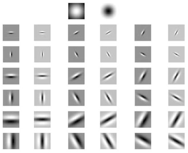
M8 filter bank. There are total of 38 filters from which two filters are rotationally symmetric (Gaussian and Laplacian of Gaussian) and the remaining 36 filters are edge and bar filters at three different scales

We analyze the texture of cytoplasm and nucleus independently. A few random cell images (n_s = 30) are selected from each class and filter responses inside the segmentation mask are clustered using k-means clustering algorithm with k_m = 30. The clustering is performed separately for pixels inside the nucleus and cytoplasm, and repeated for each disease class. Since the size and the variability of cytoplasm texture is less than the nucleus texture, we generate half the number of clusters from the cytoplasm than from the nucleus. We concatenate the cluster centers from each class and construct the texton libraries separately for cytoplasmic and nuclear texture. The algorithm for texton library generation is given in Fig. 4.

Fig. 4.

Texton library generation

Using the constructed texton library, the cells are represented with their texton histograms. Given an arbitrary cell image, the pixels inside the cytoplasm and nucleus are filtered and the responses are quantized to the nearest textons in the library. As a result each cell image is represented with two texton histograms of sizes c·k_m and c·k_m/2 corresponding to nuclear and cytoplasmic texture. The texton library generation and cell representation process is illustrated in Fig. 5.

Fig. 5.

Texton library generation and cell representation. Black and gray vectors correspond to nuclear and cytoplasmic features respectively

4 Classification

We utilize support vector machines (SVMs) to classify among four types of malignancies and normal cells. SVMs were first introduced in [6] for binary classification problems. The technique is a generalization of linear decision boundaries where decision surface is constructed in a large transformed version of the original feature space.

We first focus on the binary classification problem (c = 2). Let {(x_i, y_i)}_{i = 1, …, n} be the training set with the respective class labels, where x_i ∈ℝ^p and y_i ∈{± 1}. The SVM solves the following optimization problem

$$\begin{array}{l}\underset{\mathit{\beta },{\beta }_0,{\xi }_i}{min}\left[\frac{1}{2}{\mathit{\beta }}^{\text{T}}\mathit{\beta }+\gamma \sum _{i=1}^n{\xi }_i\right]\text{subject}\text{to}\\ y_i(h{({\mathbf{x}}_i)}^{\text{T}}\mathit{\beta }+{\beta }_0)\ge 1-{\xi }_i{\xi }_i>0i=1,\dots ,n\end{array}$$ (4)

where the training samples are mapped to an enlarged space with the function h(x). Minimizing β^Tβ is equivalent to maximizing the margin between the positive and negative samples and γ is the tradeoff between the training errors {xi;_i}_{i = 1, …, n} and the margin. We maximize the dual problem of (4) since it is a simpler convex quadratic programming problem. The dual problem and the decision function involve mapping h(x) through an inner product, therefore it suffices to define the inner product through a kernel function without defining the mapping. In our implementation we use the linear kernel function, i.e., K(x,x′) = x·x′. A more detailed discussion on SVMs can be found in [8].

Next we focus on the multi-class classification problem. The first group of methods construct several binary classifiers and combines them to solve multiclass classification problem. The most popular two methods are one-against-one and one-against-all classifiers. In one-against-one classifier, a binary classifier is trained for all combinations of classes. Then, the label of a test example is predicted by the majority voting among the classifiers. In one-against-all classifier, for each class a binary classifier is trained by labeling the samples from the class as positive examples and samples from the other classes as negative examples. A query point is assigned to the class having maximum decision function among all the classes.

The second group of methods considers all the classes together and solves the multi-class problem in one step. Due to a large scale optimization problem, these methods are computationally more expensive which makes them unsuitable for large size applications. A detailed comparison of multi-class SVMs can be found in [22].

In this paper we utilize one-against-one SVM classifier. Besides we present results for one-against-all SVM classifier, kNN classifier which is widely used for texture classification problems and LogitBoost classifier which allows us to describe the uncertainty of the classification, in Sect. 5.

5 Experiments

5.1 Cell database

Immunophenotyping was used to confirm the diagnosis for a mixed set of 86 hematopathology cases: 18 MCL, 20 CLL, 9 FCC, and 39 acute leukemia. In addition there were 19 normal cases. For each case, we have varying number of cell images ranging from 10 to 90. In total we have 3,691 cell images from 105 cases. All cases originated from the archives of either City of Hope National Medical Center in California, University of Pennsylvania of School of Medicine, Spectrum Health System, Grand Rapids, MI or Robert Wood Johnson University Hospital at the University of Medicine and Density of New Jersey.

There were obvious variations in the staining characteristics of specimens among the institutions, which were introduced because of differences in manufacturers of the dyes, choices in automated stainers and due to the overall intensity variations. All of these variables led to variations in shadowing, shading, contrasts and highlighting cues providing an added challenge for the classification algorithms. Four MCL samples from different institutions are shown in Fig. 6, which demonstrates the imaging variations among different institutions.

Fig. 6.

Mantle Cell Lymphoma (MCL) samples from four different institutions. a Robert Wood Johnson University Hospital. b University of Pennsylvania of School of Medicine. c City of Hope National Medical Center in California. d Spectrum Health System, Grand Rapids, MI. The images reflect the obvious variations in imaging conditions among different institutions

Stained specimens were examined by a certified hematopathologist using an Olympus AX70 microscope equipped with a Prior 6-way robotic stage and motorized turret to locate, digitize and store specimens. The system utilizes interactive software developed in Java and C++. The imaging components of the system consist of an Intel-based workstation interfaced to an Olympus DP70 color camera featuring 12-bit color depth for each color channel and 1.45 million pixel effective resolution. Figure 7 shows samples from normal and each disorder category originated from Robert Wood Johnson hospital. As seen in the images our cell database covers a wide range of characteristics for each disease category.

Fig. 7.

Samples from normal and each disorder category from Robert Wood Johnson (RWJ) University Hospital. Even from a single institution, the samples show great variability

5.2 Test methodology

The texture statistics of the cell images from a single case are similar to each other. As a result, the division of test and training sets without obeying the separation of cells based on per case (patient), produce biased results towards better classification rates.

We perform leave one out tests in our experiments. We select all the cell images from a single case as the test set and the remaining cell images in the database as the training set. The cells from the selected case are classified using the trained classifier. Training is repeated for each case (patient). In Sect. 5.6, we also present results for tenfold cross validation, where a model can be trained using some cells of a case and used to classify some other cells of the same case. We refer to this scheme as not obeying the separation.

We present the results for two different tests: cell classification and case classification. In cell classification, we predict the label of each cell with the trained classifier. In the case classification, we assign the label of the case according to the majority voting among its cells. Notice that there are variable number of cell images per case, ranging from 10 to 90.

5.3 Filter banks

In the first experiment, we compare the texture features generated by using M8 filter bank with LM [30], S [39], M4 [44] filter banks and the local neighborhood method [45]. The LM filter bank consists of 48 anisotropic and isotropic filter: first and second derivative of Gaussians at 6 orientations and 3 scales; 8 Laplacian of Gaussian filters and 4 Gaussian filters. The S filter bank consists of 13 rotationally symmetric filters and M4 filter bank is similar to M8 filter bank except, edge and bar filters appear only at single scale.

Initially, n_s = 30 random cell images are selected from each of the five classes, and the images are convolved with the filter banks. Also, the local neighborhood based features are constructed by stacking 7 × 7 neighborhood of each pixel. We do not normalize the images while constructing local neighborhood based features since the method uses local intensity information.

For nuclear texture we use k_m = 30 cluster centers, and for the cytoplasm texture k_m = 15 cluster centers, from each class. Therefore, the texton library has 150 textons for nuclei and 75 textons for the cytoplasms, total of 225 bin histogram for each cell.

The classification performance of different features are given in Table 1. The results indicate that M8, S and LM outperforms the M4 filter bank and local neighborhood method. There are not obvious differences among the M8, S and LM filter banks. The case classification performance of LM and S filter banks are slightly better than M8 whereas cell classification performances support the inverse argument. We consider cell classification performance as more important, since cases are classified according the majority voting of the cells and a few classified/misclassified samples among a case can drastically change the result. Moreover, M8 filter bank is the most compact space which has 8 features whereas LM and S filter banks have 48 and 13 features, respectively. The clustering and quantization steps take much longer time using the later methods, e.g., 1 h for M8 versus 8 h for LM.

Table 1.

Comparison of M8 filter bank with features constructed by different filter banks and local neighborhood method. The results are ordered according to cell classification rates

	M8	S	LM	M4	Local Neigh.
Cell classification	84.45	84.04	82.64	78.98	75.62
Case classification	89.52	90.48	90.48	84.76	82.86

5.4 Classification methods

In the second experiment we compare the one-against-one SVMs with three classification algorithms: LogitBoost, one-against-all SVMs, kNN.

Nearest neighbor classifier with the χ² distance metric is the widely applied classification algorithm used with histogram based texture representation. In kNN classification [19, p. 415], the closest k_n training samples to the query point are detected and the query point is labeled with the class having the majority votes among the detected points. It is shown with the experiments that among the other possible choices for the distance function (KL-divergence, Bhattacharya distance, Euclidean distance), χ² distance performs best for the texture similarity measure. The χ² distance between two one-dimensional histograms h₁ and h₂ is measured as

$${\chi }^2(h_1,h_2)=\frac{1}{2}\sum _{t=1}^p\frac{{(h_1(t)-h_2(t))}^2}{h_1(t)+h_2(t)}.$$ (5)

We select the optimum value of the number of neighbors parameter as k_n = 15, via cross-validation. Since χ² distance measures dissimilarity between two distributions we do not normalize each feature to have zero mean standard deviation for kNN classification, where as we perform normalization for other methods.

The second method, for comparison is multiclass LogitBoost classifier [13]. LogitBoost algorithm learns an additive multiple logistic regression model by minimizing negative log likelihood with quasi-Newton iterations. The probability of a sample x being in class l is given by

$$p_l(\mathbf{x})=\frac{e^{F_l(\mathbf{x})}}{{\sum }_{j=1}^c{e}^{F_j(\mathbf{x})}}\sum _{j=1}^c{F}_j(\mathbf{x})=0$$ (6)

where F_l(x) is an additive function

$$F_l(\mathbf{x})=\sum _{m=1}^M{f}_{ml}(\mathbf{x}).$$ (7)

At each boosting iteration m, the algorithm learns the weak classifiers f_mj(x), j = 1, …, c by fitting weighted least squares regressions of training points x_i, i = 1, …, n to response values z_ij with weights w_ij where

$$z_{ij}=\frac{y_{ij}^{\ast }-p_j({\mathbf{x}}_i)}{p_j({\mathbf{x}}_i)(1-p_j({\mathbf{x}}_i))}{w}_{ij}=p_j({\mathbf{x}}_i)(1-p_j({\mathbf{x}}_i))$$ (8)

and $y_{ij}^{\ast }$ is the binary class indicator such that $y_{ij}^{\ast }=1$ if class of i-th sample y_i = j, and 0 otherwise.

We utilize regression stumps as weak learners, which are regression trees with a single split

$$f(\mathbf{x})=\{\begin{array}{ll}a\hfill & \text{if}{\mathbf{x}}^t<\theta \hfill \\ b\hfill & \text{else}.\hfill \end{array}$$ (9)

We learn the regression coefficients a, b, the threshold θ while x^t denotes the t-th dimension among the 225 dimensions of the feature vector x. In our implementation we performed M = 300 boosting iterations. We refer readers to [13] for more technical details.

For SVM classifiers we use linear kernel and a soft penalty (γ = 0.01) for training errors [26, Chap. 11]. The classification rates are given in Table 2. Results indicate that we achieve major improvements over the widely used kNN based texture classifier with the introduction of SVMs or LogitBoost. The one-against-one SVM and LogitBoost classifiers produced comparable results, while outperforming the other methods significantly. The performance of one-against-one SVM classifier is better than LogitBoost classifier in cell classification. However, LogitBoost has certain advantages over SVM. In medical applications, it is also important to report the uncertainty about an estimation. Since LogitBoost classifier estimates the posterior distribution of class labels through (6), with this method we can describe the uncertainty of the estimation for each individual cell. In our application, we utilize one-against-one SVM classifier since it produces most accurate results.

Table 2.

Cell and case classification rates of different classification algorithms

	One-Ag.-One SVM	LogitBoost	One-Ag.-All SVM	kNN
Cell classification	84.45	83.14	81.60	81.17
Case classification	89.52	89.52	87.62	84.76

We achieve very successful results since even the most experienced doctors can predict the correct label after investigating several other medical records besides images. In a similar setup, but including fewer cases from normal and three lymphoproliferatie disorders (four class problem), three different human experts could only classify less than 70% of the cells correctly [5], which illustrates the superior performance of our approach.

In Tables 3 and 4 we present the confusion matrices for cell and case classification using one-against-one SVM. The rows of the table show the actual cell classes and the columns show the predicted cell classes. The normal and acute cells are classified accurately, whereas there is some confusion among CLL, MCL and FCC cells. In the case classification almost all of the classes are predicted correctly, and only FCC cases have several misclassifications. This is mainly because we have limited number of training examples from the FCC cases.

Table 3.

Confusion matrix of cell classification for one-against-one SVM

	Normal	CLL	MCL	FCC	Acute leukemia
Normal	734	64	11	1	0
CLL	35	504	49	63	0
MCL	11	78	375	27	67
FCC	14	62	31	132	2
Acute Leukemia	0	0	59	0	1,372

Table 4.

Confusion matrix of case classification for one-against-one SVM

	Normal	CLL	MCL	FCC	Acute leukemia
Normal	19	0	0	0	0
CLL	0	18	1	1	0
MCL	0	2	14	0	2
FCC	2	1	1	5	0
Acute Leukemia	0	0	1	0	38

Besides five class classification problem, we diagnosed the cells and the cases as normal versus disorder. Since the problem is binary classification, one-against-one and one-against-all SVMs reduced to binary SVM classifier. The classification rates both for cells and cases are given in Table 5. The results indicate that we can diagnose a case as being normal or disorder almost perfectly, only a single case is misclassified among the whole database.

Table 5.

Normal vs. disorder classification rates

	SVM	LogitBoost	kNN
Cell classification	98.09	97.13	96.29
Case classification	99.05	99.05	99.05

5.5 Other features

In the third experiment we compared the texture based representation with several other features that are commonly used for hematopathology diagnoses. The first set of features are related to area of the cell. We use nucleus and cytoplasm area and nucleus/cytoplasm area ratio. The second set of features are related to the shape of the nucleus. We analyze the shape of the nucleus based on elliptic Fourier descriptors [27] which are made invariant to changes in location, orientation and scale [5]. We achieve rotation invariance by compensating for the arbitrary position of the starting point on the contour and for the arbitrary orientation of the contour. Scale invariance is achieved by normalizing each Fourier coefficient. The following conditions are considered.

• If the first harmonic locus is an ellipse, the rotation is defined relative to the semi-major axis of the locus and we normalize the coefficients by the magnitude of the semi-major axis.

• If the first harmonic locus is circular, the rotation is made with respect to the line defined by the centroid of the contour and the most distant point on the contour and we normalize the coefficients by magnitude of the radius.

We obtain translational invariance by removing the DC coefficient from the Fourier series. We retrieve 16 harmonics (64 coefficients) for the shape of each nucleus.

We present the one-against-one SVM classification results for each of the features and the combination of all the features in Table 6. For the combined features we stack all the features into an array. We see that neither area based nor shape based features are alone enough to perform classification. The texture based features outperform both of the other features significantly. Notice that, although indirectly, the area information is presented inside the texture features, since each bin of the texton histogram is equal to the number of occurrence of the texton in the image. There are minor improvements from texture based representation, 84.45%, to combined features, 84.62%, in cell classification and 89.52–91.42% in case classification.

Table 6.

Classification rates, based on area, shape, texture and combined features utilizing one-against-one SVMs

	Shape	Area	Texture	Combined
Cell classification	47.43	66.96	84.45	84.62
Case classification	50.47	70.48	89.52	91.42

The distribution of the classification performances according to different disorders show variation from texture based features to combined features. The confusion matrix of case classification using combined features are given in Table 7. Usually in the advanced stages of FCC the nuclei show variability from the other diseases. We see that two more FCC cases are correctly classified with combined features relative to Table 4. The results almost did not affect the other classes which supports the claim. We achieve only minor improvements over the texture features with the introduction of morphological features such as area and shape.

Table 7.

Confusion matrix of case classification using combined features utilizing one-against-one SVMs

	Normal	CLL	MCL	FCC	Acute Leukemia
Normal	19	0	0	0	0
CLL	0	18	1	1	0
MCL	0	2	14	0	2
FCC	1	0	1	7	0
Acute leukemia	0	0	1	0	38

5.6 Comparison with previous method

In this section we compare our approach with the method of [5]. The problem considered in [5] is a subset of our problem, where only four classes are considered (Normal, MCL, FCC, CLL). The cell database of [5] contains only 261 specimens and the testing is performed by adopting tenfold cross validations which do not obey separation based on patient.

The results of [5] is given in Table 8. To directly compare our results with [5] and illustrate the effect of test methodology, we also performed tenfold cross validations and presented the cell classification results in Table 9. Even though the problem that we solve is more difficult (one more class), we see that our results are significantly better than [5] except for FCC class. Only the classification of FCC cells were slightly better in [5], but we note that there were only 20 FCC cells in their experiments.

Table 8.

Confusion matrix of cell classification rates of [5]

	Normal	CLL	MCL	FCC	No decision
Normal	73.0	13.4	0.0	12.0	1.6
CLL	7.0	83.9	7.1	2.0	0
MCL	0	13.6	83.3	1.4	1.7
FCC	5.0	2.5	0.0	90.0	2.5

Table 9.

Confusion matrix of cell classification rates using tenfold cross validation utilizing one-against-one SVMs

	Normal	CLL	MCL	FCC	AML
Normal	96.2	3.4	0.4	0.0	0.0
CLL	2.9	90.4	3.9	2.8	0
MCL	1.5	6.0	83.6	1.5	7.4
FCC	1.9	9.7	6.2	81.4	0.8
AML	0.0	0.0	1.4	0.0	98.9

The classification rates of our method with tenfold cross validation tests are significantly higher than the leave-one-out tests performed previously. The cell classification rate changed from 84.45 to 93.18%. We see that the separation of training and test sets without obeying case separation, produces biased results towards better performances. The specimens from a single case may have similarities to each other, which are uncorrelated to the class of the disorder.

6 Discussion

In many areas of pathology, the intrinsic variability in diagnostic complexity is compounded by a continuing lack of standard criteria for the identification of diseases and their histologic features. In the case of some lymphoproliferative disorders, most pathologists have the opportunity to review such a limited number of cases. There exists a striking disparity between the diagnoses of an expert in hematopathology and the pathologists in community hospitals. Using advanced imaging and computational tools might potentially enable investigators to detect and track subtle changes in measurable parameters.

As part of our ongoing PathMiner project, we have already described the design, development, and evaluation of an Image Guided Decision Support system for unsupervised imaging, analysis, and archiving of hemapathology specimens [4, 5, 49]. In our studies, nuclear texture was shown to be the most important discriminating feature for discriminating among a set of malignant lymphomas and leukemia which can sometimes be confused with one another during routine microscopic evaluation [12]. In the current paper we have investigated the statistical optimization of the underlying algorithms. Our experiments focused on the utilization of SVMs. Even with the inherent difficulties in differentiating among the disorders under study, classification results throughout our studies using texton histogram representation showed performance improvement through introduction of new classifiers. We achieve very successful results considering the difficulty of the problem.

The literature ascribes much of the difficulty in rendering consistent evaluation of expression patterns in cancer tissue microarrays to subjective impressions. When characterizations are based upon computer-aided analysis, objectivity reproducibility and sensitivity improve considerably. Encouraged by the results generated during the course of our studies we plan to explore the use of texture information for discriminating between healthy and cancerous tissues in immunofluorescing pathology specimens including cancer tissue microarrays.

7 Originality and contribution

This study describes a texture based solution which distinguishes between normal cells and four different hematologic malignancies. A new representation for cell images is introduced utilizing texture features. The texton libraries for cytoplasmic and nuclear components of the cell images are constructed and images are represented with two histograms corresponding to both regions.

Utilizing SVMs with the proposed representation, significant classification improvements are observed over the existing texture classification techniques. It is also shown that using multiclass LogitBoost algorithm, it is possible to infer about the uncertainty of the estimation without decreasing the performance significantly.

Experiments are conducted on a cell database consisting of samples from four different hospitals, 105 cases and 3,691 cell images. The database covers wide range of characteristics for each disorder class and includes obvious variations in the imaging conditions among different institutions. Detailed experiments are reported comparing the proposed approach with the selection of other features and classification techniques that are commonly used in hematopathological diagnosis, and the existing methods on the similar problems.

Biographies

Oncel Tuzel received the B.S. degree in 1999 and the M.S. degree in 2002 from Middle East Technical University, Ankara, Turkey, both in Computer Engineering. He is currently a PhD student in the Department of Computer Science at Rutgers University, Piscataway, NJ. His research interests are in computer vision, computer graphics, machine learning, and statistical pattern recognition. He is a student member of IEEE and the IEEE Computer Society.

Lin Yang received the B.S. degree in Electrical and Communication Engineering from Xian Jiaotong University, Xian, Shaanxi, P.R. China in 1999 and the M.S. degree in Signal and Information Processing from the Image Processing Center of Xian Jiaotong University, Xian, Shaanxi, P.R. China in 2002. He is currently working toward the Ph.D. degree in the Department of Electrical and Computer Engineering, Rutgers University at New Brunswick, Piscataway, NJ. His research interests include the development of robust image segmentation and registration, computer vision, statistics pattern recognition, content-based image retrieval and intelligent large-scale multimedia database.

Peter Meer received the Dipl. Engn. degree from the Bucharest Polytechnic Institute, Romania, in 1971, and the D.Sc. degree from the Technion, Israel Institute of Technology, Haifa, in 1986, both in electrical engineering. Between 1986 and 1990 he was Assistant Research Scientist at the Center for Automation Research, University of Maryland at College Park. In 1991 he joined the Department of Electrical and Computer Engineering, Rutgers University, Piscataway, NJ and is currently a Professor. He was an Associate Editor of the IEEE Transaction on Pattern Analysis and Machine Intelligence between 1998 and 2002. His research interest is in application of modern statistical methods to image understanding problems.

David J. Foran received a Bachelors degree in Zoology and Physics from Rutgers University in 1983 and subsequently served as a teaching assistant in the Physics department at New Jersey Institute of Technology. Between 1986 and 1988 he worked as a junior scientist at Johnson & Johnson Research, Inc. before earning his doctorate, jointly, from Rutgers University and the University of Medicine & Dentistry of New Jersey in 1992. Dr. Foran is a Professor of Pathology & Radiology and Director of the Center for Biomedical Imaging & Informatics at UMDNJ-Robert Wood Johnson Medical School and The Cancer Institute of New Jersey.

References

- 1.Aisenberg A. Coherent view of non-Hodgkin’s lymphoma. J Clin Oncol. 1995;13:2656–2675. doi: 10.1200/JCO.1995.13.10.2656. [DOI] [PubMed] [Google Scholar]
- 2.Chabat F, Yang G, Hansell D. Obstructive lung diseases: texture classification for differentiation at CT. Radiology. 2003;228:871–877. doi: 10.1148/radiol.2283020505. [DOI] [PubMed] [Google Scholar]
- 3.Chan J, Banks P, Cleary M, Delsol G, De Wolf-Peeters C, Falini B, Gatter K, Grogan T, Harris N, Isaacson P. A revised European-American classification of lymphoid neoplasms proposed by the international lymphoma study group—a summary version. Am J Clin Pathol. 1995;103:543–560. doi: 10.1093/ajcp/103.5.543. [DOI] [PubMed] [Google Scholar]
- 4.Chen W, Meer P, Georgescu B, He W, Goodell LA, Foran D. Image mining for investigative pathology using optimized feature extraction and data fusion. Comput Methods Programs Biomed. 2005;79:59–72. doi: 10.1016/j.cmpb.2005.03.006. [DOI] [PubMed] [Google Scholar]
- 5.Comaniciu D, Meer P, Foran D. Image-guided decision support system for pathology. Mach Vis Appl. 1999;11:213–224. [Google Scholar]
- 6.Cortes C, Vapnik V. Support vector networks. Mach Learn. 1995;20:273–297. [Google Scholar]
- 7.Cotran R, Kumar V, Collins T, Robbins S. Pathologic basis of disease. 5. W.B. Saunders Company; Philadelphia: 1994. [Google Scholar]
- 8.Cristianini N, Shawe-Taylor J. Support vector machines and other kernel-based learning methods. Cambridge University Press; Cambridge: 2000. [Google Scholar]
- 9.Cula O, Dana K. 3D texture recognition using bidirectional feature histograms. Intl J Comput Vis. 2004;59(1) [Google Scholar]
- 10.Duda R, Hart P, Stork D. Pattern classification. 2. Wiley; New York: 2001. [Google Scholar]
- 11.Efros A, Leung T. Texture synthesis by non-parametric sampling. Proceedings of 7th international conference on computer vision; Kerkyra, Greece. 1999. pp. 1033–1038. [Google Scholar]
- 12.Foran D, Comaniciu D, Meer P, Goodell L. Computer-assisted discrimination among lymphomas and leukemia using imunophenotyping, intelligent image repositories and telemicroscopy. IEEE Trans Inform Tech Biomed. 2000;4:265–273. doi: 10.1109/4233.897058. [DOI] [PubMed] [Google Scholar]
- 13.Friedman J, Hastie T, Tibshirani R. Additive logistic regression: a statistical view of boosting. Ann Stat. 2000;28(2):337–407. [Google Scholar]
- 14.Galloway R. Texture analysis using gray level run lengths. Comput Graphic Image Process. 1975;4:172–179. [Google Scholar]
- 15.Garcia-Conde J, Cabanillas F. Cell lymphoma: a lymphoproliferatie disorder associated with aberrant function of the cell cycle. Leukemia. 1996;10:78–83. [PubMed] [Google Scholar]
- 16.Haralick R. Statistical and structural approaches to texture. IEEE. 1979;67:786–804. [Google Scholar]
- 17.Haralick R, Shanmugam K, Dinstein I. Textural features for image classification. IEEE Trans Syst Man Cybern. 1973;3:610–621. [Google Scholar]
- 18.Hassan K, Tweed T, Miguet S. A multi-resolution approach for content-based image retrieval on the grid-application to breast cancer detection. Methods Inform Med. 2005;44:211–214. [PubMed] [Google Scholar]
- 19.Hastie T, Tibshirani R, Freidman J. The elements of statistical learning. Springer; Heidelberg: 2001. [Google Scholar]
- 20.Heeger D, Bergen J. Pyramid-based texture analysis/synthesis. SIGGRAPH ’95: proceedings of the 22nd annual conference on computer graphics and interactive techniques; 1995. pp. 229–238. [Google Scholar]
- 21.Hertzmann A, Jacobs C, Oliver N, Curless B, Salesin D. Image analogies. SIGGRAPH ’01: proceedings of the 28th annual conference on computer graphics and interactive techniques; 2001. pp. 327–340. [Google Scholar]
- 22.Hsu C, Lin C. A comparison of methods for multiclass support vector machines. IEEE Trans Neural Netw. 2002;13:415–425. doi: 10.1109/72.991427. [DOI] [PubMed] [Google Scholar]
- 23.Huang Y, Chen J, SWC Diagnosis of hepatic tumors with texture analysis in nonenhanced computed tomography images. Acad Radiol. 2006;13:713–720. doi: 10.1016/j.acra.2005.07.014. [DOI] [PubMed] [Google Scholar]
- 24.Ikeda T, Hagiwara M. Content-based image retrieval system using neural networks. Int J Neural Syst. 2000;10:417–424. doi: 10.1142/S0129065700000326. [DOI] [PubMed] [Google Scholar]
- 25.Jaulent M, Le Bozec C, Cao Y, Zapletal E, Degoulet P. AMIA symposium. 2000. A property concept frame representation for flexible image-content retrieval in histopathology databases; pp. 379–383. [PMC free article] [PubMed] [Google Scholar]
- 26.Joachims T. Making large-scale SVM learning practical. advances in kernel methods—support vector learning. MIT Press; Cambridge: 1999. [Google Scholar]
- 27.Kuhn F, Giardina C. Elliptic Fourier features of a closed contour. Comput Graphics Image Process. 1982;18:236–258. [Google Scholar]
- 28.Le Bozec C, Zapletal E, Jaulent MHD, Degoulet P. Towards content-based image retrieval in a his-integrated pacs. AMIA symposium. 2000:477–481. [PMC free article] [PubMed] [Google Scholar]
- 29.Lehmann T, Wein B, Dahmen J, Bredno J, Vogelsang F, Kohnen M. Content-based image retrieval in medical applications: a novel multistep approach. Proceedings of SPIE: storage and retrieval for media databases 2000. 2000;3972:312–320. [Google Scholar]
- 30.Leung T, Malik J. Recognizing surfaces using three-dimensional textons. Proceedings of 7th international conference on computer vision; Kerkyra. 1999. pp. 1010–1017. [Google Scholar]
- 31.Mao J, Jain A. Texture classification and segmentation using multiresolution simultaneous autoregressive models. Pattern Recogn. 1992;25:173–188. [Google Scholar]
- 32.Mavroforakis M, Georgiou H, Dimitropoulos N, Cavouras D, Theodoridis S. Mammographic masses characterization based on localized texture and dataset fractal analysis using linear, neural and support vector machine classifiers. Artif Intell Med. 2006;37:145–162. doi: 10.1016/j.artmed.2006.03.002. [DOI] [PubMed] [Google Scholar]
- 33.Mudigonda N, Rangayyan R, Desautels J. Gradient and texture analysis for the classification of mammographic masses. IEEE Trans Med Imaging. 2000;19:1032–1043. doi: 10.1109/42.887618. [DOI] [PubMed] [Google Scholar]
- 34.Nielsen B, Albregtsen F, Danielsen H. Low dimensionality adaptive texture feature vectors from class distance and class difference matrices. IEEE Trans Med Imaging. 2004;23:73–84. doi: 10.1109/TMI.2003.819923. [DOI] [PubMed] [Google Scholar]
- 35.Nielsen B, Danielsen H. Prognostic value of adaptive textural features—the effect of standardizing nuclear first-order gray level statistics and mixing information from nuclei having different area. Cellular Oncol. 2006;28:85–95. doi: 10.1155/2006/370173. [DOI] [PMC free article] [PubMed] [Google Scholar]
- 36.Rajesh L, Pattari SGG, Dey P, Srinivasan R. Image morphometry of acute leukemias. comparison between lymphoid and myeloid subtypes. Anal Quant Cytol Histol. 2004;26:57–60. [PubMed] [Google Scholar]
- 37.Ricketts I, Banda-Gamboa H, Cairns A, Hussein K. Automatic classification of cervical cells-using the frequency domain. IEE coll on app of im proc in mass health screening. 1992;9:1–4. [Google Scholar]
- 38.Rozman C, Montserrat E. Chronic lymphocytic leukemia. New Engl J Med. 1995;333:1052–1057. doi: 10.1056/NEJM199510193331606. [DOI] [PubMed] [Google Scholar]
- 39.Schmid C. Constructing models for content-based image retreival. Proceedings of IEEE conference on computer vision and pattern recognition; Kauai. 2001. pp. 39–45. [Google Scholar]
- 40.Schmid K, Angerstein N, Geleff S, Gschwendtner A. Quantitative nuclear texture features analysis confirms who classification 2004 for lung carcinomas. Modern Pathol. 2006;19:453–459. doi: 10.1038/modpathol.3800541. [DOI] [PubMed] [Google Scholar]
- 41.Schnorrenberg F, Pattichis C, Schizas C, Kyriacou K. Content-based retrieval of breast cancer biopsy slides. Technol Health Care. 2000;8:291–297. [PubMed] [Google Scholar]
- 42.Sheshadri H, Kandaswamy A. Experimental investigation on breast tissue classification based on statistical feature extraction of mammograms. Comput Med Imaging Graph. 2007;31:46–48. doi: 10.1016/j.compmedimag.2006.09.015. [DOI] [PubMed] [Google Scholar]
- 43.Vadlamudi G. Leukemic phase of mantle cell lymphoma: two case reports and review of the literature. Arch Pathol Lab Med. 1996;120:35–40. [PubMed] [Google Scholar]
- 44.Varma M, Zisserman A. Statistical approaches to material classification. Proceedings of 7th European conference on computer vision; Copehagen, Denmark. 2002. [Google Scholar]
- 45.Varma M, Zisserman A. Texture classification: are filter banks necessary?. Proceedings of 9th international conference on computer vision; Nice, France. 2003. pp. 691–698. [Google Scholar]
- 46.Walker R, Jackway P. Statistical geometric features-extensions for cytological texture analysis. Proceedings of 13th international conference on pattern recognition; 1996. pp. 790–794. [Google Scholar]
- 47.Wyszecki G, Stiles W. Concepts and methods, quantitative data and formulae. Wiley; New York: 1982. [Google Scholar]
- 48.Xu C, Prince J. Snakes, shapes, and gradient vector flow. IEEE Trans Image Process. 1998;7(3):359–369. doi: 10.1109/83.661186. [DOI] [PubMed] [Google Scholar]
- 49.Yang L, Meer P, Foran D. Unsupervised segmentation based on robust estimation and color active contour models. IEEE Trans Inform Technol Biomed. 2005;9:475–486. doi: 10.1109/titb.2005.847515. [DOI] [PubMed] [Google Scholar]