

Abstract
A novel method we refer to as the tie-line field (TLF) method has been developed to globally determine the tie-lines of any three-component two-phase coexistence region by fitting electron-spin resonance (ESR) spectra obtained from compositions on the coexistence curve and within the coexistence region. The TLF method is illustrated by applying it to the liquid-ordered (Lo) and liquid-disordered (Ld) phase coexistence region of the lipid system brain-sphingomyelin/dioleoylphosphatidylcholine/cholesterol (SPM/DOPC/Chol), for which an estimate of a tie-line was previously obtained by an earlier method also using ESR spectra. The essential aspect of the TLF method is the unique parameterization of the coexistence region called a “ruled surface”. The use of the ruled surface enables one to guarantee that tie-lines do not cross, as required by the phase rule, whereas previous methods lack this important constraint. It also makes simultaneous use of the full data set in determining the TLF and leads to a more efficient experimental design than previously used. The method is first tested out on synthetic data sets, then least-squares fitting of the ESR spectra with the parameterized model results in a tie-line field consistent with other known information on this lipid system. The best-fit tie-line field consists of the set of tie lines which are not exactly parallel; they exhibit a gradual change in slope with the largest slope within the coexistence region connecting the coexistence curve compositions with the highest and lowest cholesterol concentrations. The results are compared with those from more constrained methods of representing the tie-line fields as well as with the previous tie-line determination for the SPM/DOPC/Chol system. An accurate determination of the tie-line field of phase coexistence regions in lipid systems is a necessary step in determining coexisting lipid compositions to serve as models of cell plasma membranes.
I. Introduction
In this paper we introduce a new method for determining tie-lines in two-phase regions of multi-component model membrane systems. This work grew out of our previous work on the development of a simple methodology for using ESR spectra for this purpose (1, 2) which was recently applied to the two-phase liquid-ordered (Lo) + liquid-disordered (Ld) coexistence region of the three component SPM/DOPC/cholesterol (SPM = brain sphingomyelin, DOPC = dioleoylphosphatidylcholine) lipid system (2, 3). The limitations of that method, which independently seeks out each individual tie-line from a set of trial tie-lines, became clear and motivated us to find a more global approach using ESR spectra that removes the weaknesses of the earlier approach. These weaknesses include inefficient use of the experimental data, difficulty in constraining the individual tie-lines from intersecting, and overcoming uncertainties in some details of relevant features of the phase diagram. After developing this method herein, we illustrate its use for the two-phase Lo + Ld coexistence region of SPM/DOPC/chol, which then enables us to compare with results obtained with the earlier method (2).
In sub-section A of this Introduction we provide a review of the relevant background, and in sub-section B we introduce key aspects of the new methodology.
A. Phase diagrams and tie-lines
Phase science, the study of phase behavior, traces it roots to the development of equilibrium thermodynamics over a hundred years ago. Most of this early work was focused on one-component (pure) systems, typically gases, and their changes in state, including the phase state, with changing pressure and temperature. Phase science originated from Gibbs' studies of the equilibrium thermodynamics of mixtures with the phase rule and the concept of chemical potential; Van der Waals' equation of state, and Korteweg's theory of plaits. However, with the advent of quantum and statistical mechanics, work in phase science shifted more to the molecular understanding of phase structure and critical phenomena. Theoretical study of multi-component multi-phase systems was modest. However, experimental work into phase behavior, aided by regular binary solution theories, blossomed because of the huge industrial and practical applications, especially in materials science, colloid and interface science, and chemical engineering. But for more complex chemical systems of interest, specifically in biology, a better understanding of phase science and the thermodynamics of mixing has been necessary.
As is well-known, the phase behavior of a system is defined by stating the number, composition, and nature of the coexisting phases (4). Phase diagrams graphically depict phase behavior in terms of the state variables, such as mole fractions of the chemical constituents, temperature, or pressure. Coexistence curves divide the phase diagram into coexistence regions, which contain compositions at which the system phase separates into two or more phases. Therefore, a coexistence region is labeled by the number of coexisting phases, such as a two-phase region or three-phase region. A coexistence curve is also called a connodal because the curve is the locus of connodes, which are the compositions of the coexisting phases (5). For two-phase regions the coexistence curve is divided into two phase boundaries, with each phase boundary the locus of connodes for that particular phase. A line passing through the coexistence region and connecting the two coexisting connodes is called a tie-line. Therefore, since there are an infinite number of connodes on each phase boundary, any two-phase region is divided up into an infinite number of tie-lines, called a tie-line field (TLF).
Lipid phase behavior has been studied for many years because of its importance to the structure and function of cell membranes (6-9). The hundreds of different amphiphilic lipids varying in size and polarity yield an astonishing array of different phases when mixed with water. In particular, lipid bilayers exhibit two-dimensional phases called lamellar phases which are relevant biologically. At, or near room temperature and pressure, pure saturated phospholipid systems are naturally either in a liquid-disordered phase (called Ld) or a gel phase (called So for solid-ordered or Lβ) depending on acyl chain length. Pure unsaturated phospholipid systems can exist in either phase depending on the type of unsaturation (trans or cis carbon double bonds) but generally exist in the Ld phase, although they can form gels at lower temperatures. At much higher temperatures than room temperature, all phospholipids will generally decompose into lysolipids and fatty acids before mixing appreciably with water, reflecting the strong hydrophobic effect that leads to bilayer formation.
The lamellar, isobaric phase diagrams of binary mixtures of unsaturated and saturated phospholipids, with mole fraction and temperature as the state variables, generally show a two-phase coexistence region of Ld and gel phases within some range of temperatures. The tie-line fields for these phase diagrams are immediately known, since all tie-lines are perpendicular to the vertical temperature axis (parallel to the mole fraction axis) because of thermal equilibrium (ref 10 and references therein). According to Gibbs' phase rule for binary phospholipid mixtures with variable temperature, a three-phase eutectic point may exist, most likely, at lower temperatures, consisting of two solid phases and a liquid phase, but this has only been observed in a few mixtures. However, mixtures of gel-favoring phospholipids and cholesterol do tend to show eutectic behavior, and the addition of cholesterol to either pure phospholipid systems or binary phospholipid mixtures results in a third lamellar phase, called a liquid-ordered phase (Lo), with physical properties in-between Ld and gel phases. Also, according to Gibbs' phase rule, at constant temperature and pressure a three-component lipid mixture consisting of two phospholipids, one Ld-favoring and the other gel-favoring, plus cholesterol can exhibit three-phase coexistence with variable mole fractions. This three-phase coexistence region is a triangle in the phase diagram with each vertex representing the composition of the Ld, gel, or Lo phase. Coexistence regions and three-phase triangles have been confirmed for the distearoylphosphatidylcholine(DSPC)/DOPC/cholesterol (11) and the dipalmitoylphosphatidylcholine(DPPC)/DOPC/cholesterol (12) lipid systems, and there is good evidence for a three-phase triangle in the phase diagram of the SPM/DOPC/cholesterol lipid system (3, 13, 14, and this paper).
There are many well established methods to determine accurately and precisely phase boundaries of coexistence regions in ternary lipid systems (10-12, and 15-18), which address the challenge that some systems do not exhibit bulk (visible) phase separation. These methods are essentially divided into two types, either direct observation by fluorescence microscopy or through the measurement of some signal. However, both types rely on the presence of a probe. In addition, this probe signal can be either a spectrum, which is a vectorizable function of frequency (or magnetic field) (ESR, NMR, UV/visible/IR absorbance) or a scalar value (FRET, single-dye fluorescence, fluorescence anisotropy). The direct observation method of fluorescence microscopy, while straightforward and informative, involves a sample preparation (i.e. Giant Unilamellar Vesicles, GUVs) prone to trapping metastable states. On the other hand, the signal measurement approach allows for a well-equilibrated sample preparation, but the analysis of the data depends on the application of the linear superposition model for physical properties of phase separated systems. This approach assumes that the probe partitions between the distinct (possibly sub-microscopic) coexisting phases, and only an insignificant fraction of the probe is at the interface of the phases. Therefore, because the probe is reporting on the internal physical properties of the phase, the signal from a sample within the coexistence region is a linear combination of the signals from the coexistence curve compositions at the end points of the tie-line passing thru this total composition. In general, the linear superposition approach should be accurate for probes chemically resembling lipids. Moreover its application ultimately requires knowledge of the tie-line. Two more requirements are that the signals from the phases in coexistence be significantly different from each other and that the probe's partition coefficient not be much different from unity. The linear superposition approach can be used to determine coexistence curves as well as tie-lines. However, experimentally determining tie-lines for lipid systems containing more than two lipid species has been difficult.
Recently, two methods have been published to determine individual tie-lines one at a time: the Veatch et al method (19) and the trial tie-line method (1, 2). Both methods use the linear superposition approach for magnetic resonance spectra and a specific compositional arrangement of samples in the experimental design, but they differ in applying the knowledge of the coexistence curve and in the partitioning behavior of the probe used, as well as the method to determine the coefficients of the linear superposition model. These methods have been applied to three different lipid systems. In the DPPC/DLPC/cholesterol (two saturated phospholipids/cholesterol) lipid mixture the trial tie-line method determined a coarse-grained tie-lie field one tie-line at a time and the results were consistent with what is known and expected for this system (1). On the other hand, the results for the DPPC/DOPC/cholesterol (saturated/unsaturated phospholipids/cholesterol) system using the Veatch et al method (19, 20) and the SPM/DOPC/cholesterol system (saturated/unsaturated phospholipids/cholesterol) system using the trial tie-line method (2) were expected to be similar but were not. The reasons for this were unknown but there are currently two limiting theories, one a regular solution theory involving a chemical interaction between saturated lipid and cholesterol (21) and the other is a mean-field theory involving differences in lipid packing due to the presence or absence of an unsaturated bond (22), which may offer insights. However, experimentally determined tie-line fields are needed to better understand such lipid phase behavior.
Currently, there have been no experimental methods to globally determine the tie-line field, as opposed to fitting one tie-line at a time. The procedure proposed in this work, which we call the tie-line field (TLF) method, does address this issue by globally determining the whole tie-line field within a two-phase coexistence region in lipid systems. Like the previous methods, the TLF method is based on the linear superposition of magnetic resonance spectra, but it simultaneously includes all the spectra throughout the entire composition space of the coexistence region. The method, as we have developed it, requires that the boundary of the two-phase coexistence region be known, although, in principle, it could be generalized to allow for simultaneous fitting of the phase boundaries (e.g. ref 10). The heart of the method of analysis is a unique mathematical parameterization called a ruled surface. A ruled surface is any surface composed of non-intersecting line segments and can be embedded in spaces of two (planar) or more dimensions. A simple example of a ruled surface is given by the surface of a finite but open cylinder (i.e. the parallel lines along this surface connecting the two circles forming the rims of the surface). Ruled surfaces have been long known to mathematicians. The concept of a ruled surface was introduced for two-phase coexistence regions of mixtures as a function of a single composition variable vs. temperature (23-26), where for binary mixtures the ruled surface is the set of horizontal (isothermal) line segments connecting the compositions at thermal equilibrium. However, the ruled surface parameterization has not been utilized to determine tie-line fields.
B. Key aspects of the new methodology
In this paper we simply identify as the ruled surface the planar surface corresponding to the Lo + Ld phase coexistence region (of the three component phase diagram at constant temperature), which is bounded by the coexistence curve. This surface is “ruled” by the non-intersecting tie-lines that connect the coexisting Lo and Ld phase compositions on the coexistence curve. Thus the ruled surface and the tie-line field are mathematically one and the same. That the tie-lines must not intersect follows directly from Gibbs' Phase Rule (if there were a crossing, at the point of crossing there would be four distinct compositions in equilibrium, impossible with just three components at constant temperature and pressure). This fundamental constraint of non-crossing is automatically included in our method, whereas in previous methods, which sought out individual tie-lines, it is more difficult to impose this constraint. The section of the coexistence curve representing the Lo phase boundary is taken as the function u and that for the Ld phase boundary is given by the function v.
Since each point along v is connected to a unique point along u by the tie-line, we can express v = v(u). The task of finding the tie-line field is then just to obtain v(u) from the experimental data. The non-intersection of the tie-lines merely requires v(u) to be a monotonically increasing function of u, i.e. dv/du is greater than zero. Additional constraints, e.g. starting and end-points of u and v can then be introduced in the empirical parameterization of v(u) as needed.
Another virtue of our method is that all the experimental data is fit simultaneously to obtain the complete tie-line field, once the problem is formulated as a constrained minimization, which can be solved by standard algorithms. This makes efficient use of all the experimental data. In fact, we show in this work that we can obtain the whole tie-line field with data sets no greater than what was needed to obtain a single tie-line in the previous study on the SPM/DOPC/Chol system (2). Furthermore, in that study, once each approximate tie-line is located, only a small fraction of the data set is useful in the statistics of the fitting.
It is clearly of interest to compare the performance of the new TLF method with the previous one (1, 2), which we refer to as the trial tie-line (TTL) method. It is for this reason that we have chosen the same Lo + Ld two phase region of the SPM/DOPC/Chol system to enable a direct comparison, in this first application of the TLF method. It also enables us to illustrate some other virtues of the TLF method, which were not available in the TTL method. For example, the coexistence curve encompassing such a two phase region can be challenging to obtain in all its features. While the coexistence curve for this system was determined by standard methods (3, 15) (i.e. confocal fluorescence microscopy and FRET), there is always the challenge of determining the putative critical point(s) on this curve, and, in the present case, the end tie-line which forms the phase boundary with the known three phase region. It is our purpose also to show that it is sufficient to have just approximate knowledge of these key features at the outset.
The TLF method, as we have developed it, is robust enough to also locate fairly accurately both the critical point and the end points of the phase boundary with the three phase region as part of the global fitting. This would be more difficult to accomplish by means of a TTL method, so greater initial effort is required in precisely locating these features prior to finding the tie-lines.
As in the previous studies using the TTL method with a spin-probe, such as 16PC, the analysis must also include the determination of its partition coefficient Kp between the Lo and Ld phases. Although it must be constant along a tie-line, there is no reason to assume that it is the same for all the tie-lines. However, there is every reason to suppose that it is a gently varying function of the ruled surface function u. This feature is naturally built into our new TLF method, whereas by means of a TTL method the Kp for each tie-line must be independently determined, which does not readily enable one to guarantee that it is a smoothly varying function of u. We do compare in our study the respective values of both Kp and the slope of tie-lines obtained by the TLF method vs. that previously obtained by the TTL method, where possible.
The outline of this paper is as follows: Section II provides experimental details, Section III the TLF method for fitting the data, Section IV the results of the data analysis by the TLF method, and Section V the discussion of these results. A glossary of definitions of symbols used appears in the Appendix.
II. Experiment
A. Materials
The phospholipids (SPM and DOPC) and the spin label 1-palmitoyl-2-(16-doxyl stearoyl) phosphatidylcholine (16PC) were purchased from Avanti Polar Lipids, Inc. (Alabaster, AL). Cholesterol was obtained from Sigma-Aldrich (St. Louis, MO). Stock solutions of the lipids were prepared by diluting or dissolving the shipped stock in chloroform in a sealable vial. Purity > 99% of the stock solutions was determined by thin-layer chromatography for phospholipids in chloroform/methanol/water = 65:25:4 (by volume) and hexane/diethyl ether/chloroform = 7:3:3 for cholesterol. All materials were used without further purification. The purity of stock solutions was checked every three months. The concentration of the phospholipid stock solutions was determined by a slightly modified procedure for the “determination of total phosphorous” published on Avanti Polar Lipid, Inc.'s website for technical information (http://www.avantilipids.com/TechnicalInformation.html). The concentration of the cholesterol stock solution was determined from an accurate mass (± 0.1mg) of the powdered cholesterol stock and the preparation of the solution in a 50 mL ± 0.05 volumetric flask.
B. Preparation of model membranes
Spin-labeled lipid dispersions consisting of SPM, DOPC, and cholesterol were prepared as follows. Measured volumes of lipid stocks and the spin-label stock were dispensed using a Hamilton repeating dispenser into glass test tubes using a 50 μL Hamilton syringe to give the desired lipid compositions. The concentration of spin-label in the lipid dispersion was 0.2% of the total lipids. These lipid-chloroform solutions were then converted to lipid-buffer suspensions by Rapid Solvent Exchange (27). The buffer used was 50 mM Tris, 10 mM NaCl, and 0.1 mM EDTA at pH 7.0. The samples were stored under an argon atmosphere in the dark at room temperature for at least 24 hours to reach equilibrium. Previous work on the maximum solubility of cholesterol in phospholipid bilayers (28) demonstrated that sample preparation with temperature annealing was especially important for samples with a mole fraction of cholesterol ≥ 0.5, even if measurements were to be performed at room temperature. However, temperature annealing was not performed in the current work because none of the samples had a mole fraction of cholesterol ≥ 0.5 and the coexisting phases studied at equilibrium were both fluid; therefore, at least a day at room temperature combined with the Rapid Solvent Exchange procedure was enough to ensure complete mixing. After a few days the samples were centrifuged and the pellets were transferred to 1.5–1.8-mm-diameter × 100-mm-length glass capillaries with excess buffer. After the samples were centrifuged in the capillaries, the supernatant (excess buffer) was removed to less than a millimeter above the pellet and the ends of the capillaries were flame sealed. The samples were not deoxygenated in a glove bag because previous work showed there was a negligible difference in 16PC X-band spectra over the relevant range of compositions. This range of compositions was determined from the phase diagram of the SPM/DOPC/Chol system (3), previously obtained using standard methods of confocal fluorescence microscopy and FRET (15), for which the Lo + Ld coexistence region was utilized in ref. (2).
C. ESR spectral collections
ESR spectra were obtained on a Bruker Instruments EMX ESR spectrometer at a frequency of 9.3 GHz at room temperature (∼23°C). The ESR capillary was placed inside a 2mm NMR tube which was marked to position the sample pellet in the middle of the resonator. This configuration allowed for efficiency and consistency in switching samples, tuning, and sample measurements. The spectrometer settings for all samples were as follows: center field = 3477 G, sweep width = 120 G, microwave power = 2 mW, modulation frequency = 100 KHz, modulation amplitude = 0.5 G, resolution (points) = 1024. The number of scans for each spectrum varied, but the all spectra were aligned with respect to magnetic field and normalized before analysis.
III. Data Fitting Method
A. Coordinate system for the Gibbs' triangle
As is well-known, the equilateral Gibbs' triangle is used to represent the compositional state of a closed ternary system and is the domain for phase diagrams of ternary mixtures (Figure 1A). Ternary mixtures are points within the triangle, binary mixtures are points on the edges, and pure states are on the vertices. The compositional state of a lipid bilayer can be represented as a vector of mole fractions:
Figure 1.

Coordinate systems to represent compositional space for ternary phase diagrams. A) The Gibbs' triangle represents mixtures of the three lipid components, brain-sphingomyelin (SPM or S), dioleoylphosphatidylcholine (DOPC or D), and Cholesterol (C), with coordinates in mole fractions. Every point within the triangle represents a ternary mixture of all three lipids. A point on an edge represents a binary mixture of either SPM/DOPC (bottom edge), DOPC/Cholesterol (left edge), or SPM/Cholesterol (right edge). The left vertex of the triangle is pure DOPC, the top vertex is pure Cholesterol, and the right vertex is pure SPM. B) The linear transformation of the Gibbs' triangle from the three-dimensional mole fraction space to the plane of the ψ-coordinate system, ψS = ξS + ξC * cos(π/3) and ψC = ξC * sin(π/3). The eS and eC are the basis vectors that span the Gibbs' triangle.
| (1) |
where and 0 ≤ ξi ≤ 1. In the summation n stands for the set of components, {S, D, C}, where S is for SPM, D is for DOPC, and C is for Cholesterol. The Gibbs' triangle lies in a three-dimensional Cartesian vector space; however, since only two of the mole fractions are independent, we can perform a linear transformation to the “ξsξc”-plane for a more convenient coordinate system ψ. This transformation is a combination of a projection and rotation (Figure 1B):
| (2) |
, where and . The basis vector eS and eC are not orthogonal but are of unit length in the Euclidean sense. In principal, any one of the three mole fractions can be eliminated resulting in different edges of the Gibbs' triangle being the basis vectors. We arbitrarily chose to eliminate the DOPC mole fraction.
B. Modeling tie-line fields
A tie-line field is the infinite number of tie-lines that partition a two-phase coexistence region. Our model of tie-line fields begins with a representation of the coexistence curve for a two-phase coexistence region. Figure 2A shows the known Lo + Ld phase coexistence boundary for the SPM/DOPC/Cholesterol ternary lipid system (3, 13, and 14). This coexistence curve is shown as a closed loop or ellipse; however, two-phase coexistence regions in ternary mixtures can have different coexistence curve shapes or configurations if they intersect a three-phase coexistence triangle or a binary edge. Coexistence regions that intersect other coexistence regions are called “open” and ones that do not are called “closed”. The “contact rule” or “boundary rule” of phase diagrams governs which type of coexistence region (i.e. two-phase, three-phase) can intersect or contact another (29, 30). Two-phase coexistence regions can only contact a one-phase region and/or three-phase triangle, and the coexistence curve has a different configuration for each combination (Figure 2B). The closed two-phase coexistence region has two critical points (Figure 2B-1). An open two-phase region (Figure 2B-2) can either contact a one-phase region with a critical point and a three-phase triangle to its edge (called an end tie-line from the two-phase perspective), or contact a three-phase triangle with one end tie-line and another three-phase triangle with another end tie-line (Figure 2B-3). Results from experiments of our own (see results in this paper) and others (3, 13, 14) have indicated that the two end tie-line coexistence curve configuration does not exist for the Lo + Ld region of SPM/DOPC/Cholesterol, but that the two critical point and one critical point + one end tie-line configurations are still possible, although the latter is believed to be more likely. Therefore, we only considered these two cases. They will henceforth be referred to as the “closed” (two critical points) and “open” (one critical point/one end tie-line) boundary configurations, but we shall emphasize our results for the latter (open) configuration.
Figure 2.
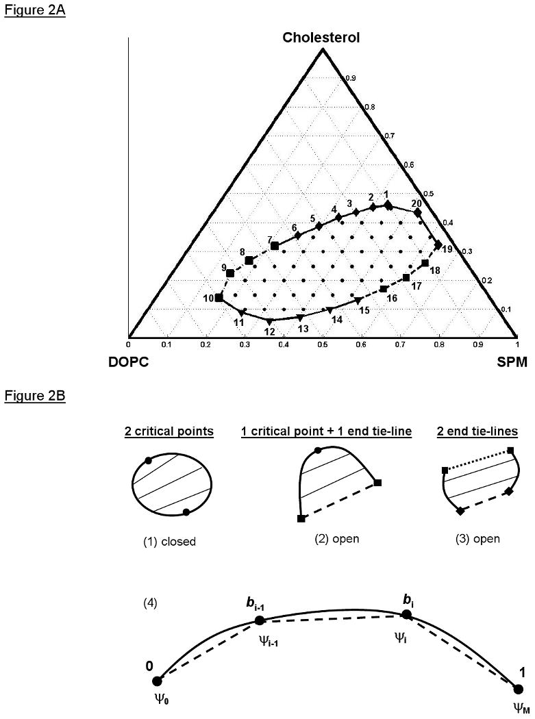
Coexistence curve configurations for two-phase coexistence regions and the chord-length parameterization of curves. A) The coexistence curve of the Lo + Ld phase coexistence region of SPM/DOPC/Chol plotted on the Gibbs' triangle (2, 3). The short dotted-dashed section at the far left of the coexistence curve indicates roughly where there is a critical point; the dashed section to the lower right indicates a region of estimated transition between the Lo + Ld two-phase region and the three-phase region (2, 3). The horizontal dotted lines represent constant cholesterol mole fractions, the 60° dotted lines represent constant SPM mole fractions, and the 120° dotted lines represent constant DOPC mole fractions. The data that is fit in the TLF method consists of compositions on the coexistence curve (20 samples connected by solid black line) and compositions within the coexistence region (51 samples, dots). Based on analysis of the 16PC ESR spectra on the coexistence curve (Figure 6A) and the outer hyperfine splittings of these spectra (Figure 6B), the coexistence curve compositions are divided into 8 Lo compositions (diamonds), 5 Ld compositions (triangles), and the 2 phase transition regions (squares). B) The coexistence curve configurations for a two-phase coexistence region showing (1) a closed configuration with two critical points, (2) an open configuration with one critical point and one end tie-line (dashed line) to a neighboring three-phase triangle, or (3) another open configuration with two end tie-lines (dashed and dotted lines) to two different three-phase triangles. (4) The chord-length parameterization of curves is an approximate arc-length parameterization. The chord-length parameters b lie on the interval [0,1]. The solid line is the real curve and the entire dashed line is its polygonal representation with M total points. The chord-length parameters are calculated from the Euclidean lengths of the individual dashed intervals (i.e. chords of the curve).
Since we initially had no knowledge of the exact location of the three-phase region, we initially utilized a closed representation of the coexistence curve; then, in our fitting of the TLF, we generated the possible open configurations by assigning the end tie-line as connecting two points on the putative phase boundary (Figure 2A). The slopes of the tie-lines in a tie-line field are bounded by such an end tie-line and by the location of (and slope of the tangent to) the critical point(s). Therefore, the coexistence curve was parameterized to enable locating these points. These boundary parameters were then used as search parameters in fitting the data to the best tie-line field.
Generally, the coexistence curve is some smooth curve and the canonical parameterization of a curve is the arc-length. However, experimentally, the coexistence curve was known as a closed set of 20 points forming a 20-sided regular convex polygon. A spline representation can be fit to this polygon, but the process of fitting a general spline to a set of points and calculating the arc-length parameterization of the resulting spline curve is nontrivial. Therefore, for simplicity, we used the polygon representation of the coexistence curve and the chord-length parameterization (Figure 2B-4) as an approximate arc-length parameterization. This enabled convenient interpolation of measured properties (i.e. ESR spectra) along the coexistence curve. The modeling of tie-line fields also requires the relationship between the compositions along a tie-line and the compositions of the connodes (end points) of that tie-line. This relationship was calculated from the conservation of matter equations between two phases and the lever rule (Figure 3). That is, in terms of the number of moles of SPM, DOPC, and Cholesterol, , and , respectively. The superscript d stands for the Ld phase and the superscript o stands for the Lo phase. These expressions are readily converted to mole fractions (ξi) by dividing through by N, the total number of moles, enabling us to write in vector form:
Figure 3.

The lever rule is the solution of the conservation of matter equations for the fraction of Lo phase (φo) and Ld phase (φd) and when the coexistence composition (ξ) and the end-point compositions (ξd and ξo) are all constrained to lie on a line (i.e. tie-line). The lever rule is essentially the parameterization of a tie-line, with the fractions of phase lying on the interval [0,1]. The lever rule is invariant under our ξ, to ψ coordinate transformation and has the form of a ratio of two Euclidean distances (x/z and y/z).
| (3) |
The coefficients φo and φd are defined as, and , where , and N = Nd + No. Therefore, φo is the fraction of the total number of moles of all lipid species that are in the Lo phase (i.e. the fraction of Lo phase), and φd is the fraction of the total number of moles of all lipid species in the Ld phase (i.e. the fraction of Ld phase). These coefficients can be calculated with the lever rule for composition ψ using the Euclidean norm as:
| (4a) |
| (4b) |
, where, and . As can be seen, the lever rule is invariant under our coordinate system transformation (as it must be) and it has the form of a ratio of two Euclidean distances. It should be noted that the lever rule is not the conservation of matter equations. The lever rule is the solution of the conservation of matter equations for the fractions of phase (φo and φd) when all compositions lie on a line (i.e. tie-line). The conservation of matter equations can still be solved for a coexistence composition that does not lie on the line connecting the end-point (phase boundary) compositions; however, in either case, the constraint that the fractions of phase sum to unity still holds. The ruled surface tie-line field is the most general way to model tie-lines. Therefore, we only discuss the implementation and results of this approach. Some comments about simpler approaches are provided in the Results Section.
A ruled surface is a surface generated by a line segment moving along a curve (31) and can have the following parameterization (32):
| (5) |
The two non-intersecting space curves A(x) and B(x) are called directrices and the line segments connecting the curves are called rulings. The directrices can either be connected or unconnected. If connected, then the directrices share a common point, if not, they are unconnected. In other words, a ruled surface is the linear combination of two different curves, and can be visualized in three dimensions as the surface formed by moving a line segment through space. Any tie-line field can be expressed as a ruled surface, where the Lo boundary and the Ld boundary are the directrices and the tie-lines are the rulings:
| (6) |
The function, v(u), is the tie-line field function (Figure 4B and 4C-1), which specifies which connode on the Ld boundary with chord-length boundary parameter v that connects to its coexisting connode on the Lo boundary with chord-length boundary parameter u. Requiring the derivative of v with respect to u to be greater than zero insures that the tie-lines do not intersect. The parameters u and v begin and end either at the critical point(s) or the end points of the end tie-line, and, in theory, can be parameters from any curve parameterization. The coexistence curve configurations for two-phase regions (Figure 2B) are shown parameterized as ruled surfaces in Figure 4A. The ruled surface parameterization for the closed coexistence curve configuration of the Lo + Ld coexistence region in the SPM/DOPC/Cholesterol system is shown in Figure 4B. The tie-line field function determines how the slopes of the tie-lines vary. We adopted a simple form (Figure 4C-2) with just a single parameter c to be fit for purposes of the present study:
Figure 4.
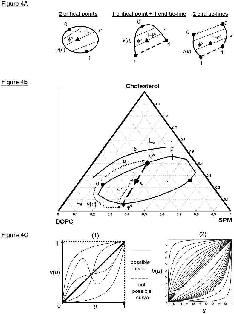
The tie-line fields of two-phase coexistence regions have a ruled surface parameterization containing a tie-line field function for specifying how the slopes of tie-lines vary across the field. A) The ruled surface parameterizations of the coexistence curve configurations represented in Figure 2B. The u chord-length parameter specifies the Lo phase composition on the Lo phase boundary (directrix) and the v chord-length parameter specifies the Ld phase composition on the Ld phase boundary (directrix). By definition, the boundary conditions v(0) = 0 and v(1) = 1 ensure that the start point of the Lo directrix connects to the start point of the Ld directrix. B) The ruled surface parameterization of the closed Lo + Ld coexistence region in the SPM/DOPC/Chol lipid system. Also shown is the total coexistence curve parameter b that specifies the location of the critical points (black squares) on the coexistence curve. C) (1) Possible (solid lines) and not possible (dashed line) functional forms for the tie-line field function v(u) of the ruled surface parameterization. (2) The tie-line field function used in our TLF method plotted with different values of the variable parameter c.
| (7) |
In Eqn 7, c > 0, v(0) = 0, and v(1) = 1. This form for v increases monotonically with u and satisfies the boundary conditions v(0) = 0 and v(1) = 1, consistent with the constraints of Eqn 6.
The essential aspect of finding the correct tie-line field for a given coexistence curve is to find the best tie-line field function v(u) using the ruled surface parameterization. Then a tie-line through a particular point in the coexistence region is the line thru this point that solves the ruled surface parameterization for the Lo boundary parameter (u), fraction of the Lo phase (φo) obtained from the lever rule, and the tie-line configuration function (v), which is also the Ld boundary parameter. Different tie-line fields are searched in the least squares fitting by varying the locations of the critical point(s) and/or end points of the end tie-line (within their range expected from experiment), which determine the end-points of the phase boundary directrices from which to calculate the chord-length parameters u and v(u), as well as by varying c. The method could, of course, be extended to more sophisticated forms of parameterization than that of Eqn 7.
C. Fitting ESR spectra
The ESR data consist of spectra obtained from known sample compositions within the two-phase coexistence region and on the coexistence curve. On the whole, the fitting method involves searching different tie-line fields, each generating trial spectra for the two-phase region by linear combination of the coexistence curve spectra, and then performing a least squares fit of these trial spectra to the experimental spectra within the coexistence region. As needed, coexistence curve spectra located at coexistence curve compositions between the known compositions at which spectra have been experimentally determined are obtained by linear interpolation. For our analysis, ESR spectra are taken as signal vectors, that is a discretization of the derivative signal versus magnetic field. Within a two-phase coexistence region the signal vector, S, at a specific bulk (total) composition is a linear combination of the coexistence curve signal vectors, Sd and So, at the endpoints of the tie-line (i.e. connodes):
| (8) |
where fd + fo = 1 and fd, fo ∈[0,1]. The coefficients fo and fd are defined as, and , where fo is the fraction of total spin-probe that is in the Lo phase and fd is the fraction of total spin-probe in the Ld phase. Through the ruled surface parameterization of tie-line fields, the linear combination of spectra can also be considered as a ruled surface:
| (9) |
However, the space of tie-line fields and the space of spectra are different, and are related through a nonlinear transformation involving the partition coefficient of the spin-probe, Kp. From the conservation of total spin-probe in the two phases and the definition of mole fractions (similar for the lipids, cf. Eqn 3, in the low concentration limit),
| (10) |
, and with the definition of Kp,
| (11) |
, the transformation between the spaces can be written as,
| (12) |
Therefore, the linear (convex) combination of spectra is from Eqn 8,
| (13) |
Eqn 13 displays the connection between the ESR data and the tie-line field via Kp.
Since the Kp is constant along a tie-line (i.e. independent of φo), the Kp across tie-lines is a function only of the Lo boundary parameter u, and its form depends on the coexistence curve configurations (i.e. open or closed) and certain boundary conditions, which are that the Kp at a critical point is unity and the Kp at an end tie-line is greater than zero. For the closed boundary case we chose the following simple form for parametrizing Kp:
| (14) |
for which Kp(0) = 1 and Kp(1) = 1 as required at the critical points. For the open boundary case, we chose this form:
| (15) |
with Kp(0) = 1 and Kp(1) > 0 ⇒ a + b > −1. The fitting parameters are “a” and “b”. We did not assume the Kp function is a second-order polynomial. We only assume that the Kp function is a smoothly-varying analytical function that obeys certain boundary conditions; therefore, the Kp function was expanded as a Taylor's series around the critical point(s). We truncated the series after the quadratic term to provide the simplest functional form that both satisfies the boundary conditions and contains a limited number of fitting parameters, along with the assumption that Kp is a slowly varying function over the range of 0≤u≤1, so higher order corrections to the expansion are small. As seen below, it provides a reasonably accurate fit to the experimental data.
In summary, predicting an ESR spectrum at a composition within the coexistence region involves determining the Lo and Ld boundary parameters u and v of the tie-line through that coexistence composition from the ruled surface parameterization of the TLF, and in addition evaluating the Kp for that tie-line using the Kp function (Eqn 14 or 15). Next, the spectra at the tie-line end-point compositions are found by interpolating the experimentally determined boundary spectra, and then the predicted spectrum at the coexistence point is calculated using Eqn 13.
At this point it is useful to compare the tie-line field (TLF) method with the tie-line determination method previously published (1), henceforth called the trial tie-line (TTL) method, because the fitting criterion we use for the TLF method in this work is based on that used in the TTL method. First, the TTL method uses the set of compositions along each of several trial tie-lines and determines which of them provides the best spectral fit, providing just a single best-fit tie-line at a time. The TLF method determines the whole TLF from the global set of coexistence samples. In the TTL method Kp is a parameter that is allowed to vary independently for each coexistence composition on a trial tie-line during the fitting of the coexistence spectrum. Then the standard deviation of this set of Kp's (i.e. σKp) along the ith TTL is used to weight the quality of the spectral fit of the TTL given by its average reduced chi-square, . Thus one has for the ith TTL the weighted or “effective” chi-square:
| (16) |
The χ2red is for one coexistence composition and the average is over all coexistence compositions on the ith TTL. Eqn 16 was utilized because it was found to yield better predictive results than finding the best fit for all spectra along the trial tie-line simultaneously with optimizing the value of Kp.
We developed our fit criterion with this observation in mind, but generalized for the TLF method. We now present the algorithm for the fitting procedure that we adopted (cf. Figure 5 which gives a flow chart):
Figure 5.

The flow chart of the TLF data fitting method showing the order and dependences of important calculations and procedures.
An arbitrary choice of critical point(s) and/or end tie-line locations is made within their expected range. In addition the TLF function v(u) is selected with an arbitrary choice of parameter c.
The ruled surface parameterization yields the ith hypothetical TLF (HTLF).
From the HTLF, determine the tie-line for the kth coexistence composition (51 total in the present study); this yields the two tie-line end-point (connode) compositions, from which φo and φd = 1- φo are determined from the lever rule (Eqn 4).
From the experimental ESR spectra along the coexistence curve determine (interpolating as needed) the ESR spectrum for each of the two tie-line end-point compositions found in step 3 for the kth coexistence composition.
-
Then for the experimental ESR spectrum at the kth coexistence composition (Sk) and the spectra at the two hypothetical tie-line end-points (Sd and So) solve the constrained least squares problem based on the linear superposition that is given by
(17a) where , to determine (and ). The vector fE contains the “estimated” fraction of total spin-probe coefficients fd,E and fo,E. These estimates are implicitly based on allowing Kp to vary independently for each coexistence composition. This “estimated” Kp can be calculated with
(17b) which is a rearrangement of Eqn 12.
-
Then one determines an “estimated” spectrum SE from
(18) for the kth coexistence composition.
-
Now for the kth coexistence composition one determines
(19) where χ2E is the chi-square between the “estimated” spectrum and the experimental spectrum for a coexistence composition. The variance of the noise (σ2) was taken from the first and last 200 points of the experimental spectrum. Then the average of χ2E or is taken over all coexistence compositions for the ith HTLF:
(20) Now an arbitrary choice is made of the parameters a (and b) in the functional form for the Kp(u) (Eqn 14 or 15) giving the jth Kp parameters. The “predicted” Kp for the kth coexistence composition is the evaluation of the Kp function using the Lo boundary parameter u for that coexistence composition. Then Eqn 13 was used to generate another set of spectra, SP, called the “predicted” spectrum for each coexistence composition using the linear combination of tie-line end-point spectra obtained from the HTLF. This SP is thus based on a “constrained” Kp(u), which is required to be constant along each tie-line. Also, the fo,P and fd,P, the “predicted” fraction of total spin-probe coefficients, are readily obtained from Eqn 12.
-
Now for the ith HTLF and jth Kp parameters obtain the norm of the squares of the differences between the fo,E and fo,P and the fd,E and fd,P given by
(21) -
From steps 7 and 9 one then forms the weighted chi-square (χ2)i,j given by
(22) for the ith HTLF and jth choice of Kp parameters.
Now minimize (χ2)i,j with respect to critical point(s) and/or end tie-line locations and the parameters a, b, and c to find the best fit TLF and Kp function consistent with the global set of ESR spectra.
-
In addition, calculate the chi-square
(23) for the kth coexistence composition, and then perform the average over the N (51 in this study) coexistence compositions to obtain given by
(24) for the ith choice of TLF and the jth choice of Kp parameters.
From a comparison of Eqn 16 from the TTL method and Eqn 22 for the TLF method, one sees that χ2E plays the role of χ2red and ‖fE−fP‖ is related to σKp. In fact, a major reason we used Eqn 22 for fitting our data was because Eqn 22, applied to find a single tie-line, yields the same answer as Eqn 16 for the best trial tie-line when analyzing the same data from the SPM/DOPC/Chol system (2). In addition, stability of the fitting was another reason we used ‖fE−fP‖ of Eqn 21 instead of the norm of the difference between “estimated” and “predicted” Kp's. Very small values of fd,E in Eqn 17b, which could occur in the TLF method, but not in the TTL method, would make the expected Kp very large. The more traditional chi-square, given by Eqn 24, was also calculated for the TLF, but did not provide sufficient stability in the fitting, in accord with the experience in Chiang et al. (1). We attribute this to the fact that the ESR spectra, for small composition displacements along either the Lo or Ld coexistence curve, typically change to a small degree, but there is considerable sensitivity to the degree to which Kp remains constant along a hypothetical tie-line. Since the fitting chi-square (Eqn 22) and the traditional chi-square (Eqn 24) are closely related, we justifiably used the traditional chi-square to statistically analyze the quality of a fit between different tie-line field models. The fitting of the ESR data with the TLF models was implemented with a program written in Matlab 7.0 R14 (The MathWorks Inc., Natick MA). The choice of search algorithm was either the constrained simplex method (“fminsearchcon” written by John D'Errico, woodchips@rochester.rr.com, released 12/16/06 and obtained from Matlab Central) or the interior-reflective Newton with a subspace trust region using preconditioned conjugate gradients (builtin Matlab 7.0 function “lsqnonlin”).
IV. Results
A. Analysis of ESR data determined phase transition regions on the coexistence curve
The data that were fit for determining the best tie-line field were the sample compositions in mole fractions and the ESR spectra obtained at those compositions. The compositions on the coexistence curve and within the Lo + Ld coexistence region of the SPM/DOPC/Chol phase diagram are shown in Figure 2A. There were 20 compositions on the coexistence curve and 51 compositions within the coexistence region. It is very desirable to determine the coexistence curve as precisely as possible. We estimate that the uncertainty in the position of the coexistence curve is no greater than 5%, which are the compositional increments of the experimental procedures (i.e. confocal fluorescence microscopy and FRET) used to determine the coexistence curve (3, 15), whereas the minimum uncertainty is no less than 1%, which is the precision of commercially available volumetric syringes for dispensing liquids that were used to prepare the samples. We estimate that the uncertainty in the composition of our samples is no greater than 2%, since our sample preparation method was optimal for minimizing this uncertainty. In publications of other phase diagrams (DPPC/DOPC/Chol and DSPC/DOPC/Chol) an uncertainty in phase boundaries of between 2% and 5% was also estimated (11, 12), and the experiments used to determine the SPM/DOPC/Chol phase diagram were similar. In our experiments, the samples within the coexistence region were selected to provide an even distribution of 5% compositional increments in sphingomyelin and cholesterol for convenience and to provide good coverage of the whole coexistence region.
All ESR spectra are from the 16PC spin-probe, which is an end-chain labeled phosphatidylcholine (1, 2). The spectra from the coexistence curve compositions are shown in Figure 6A. The transition regions were determined by visual inspection of the spectra and the outer hyperfine splittings (Figure 6B). A transition region of the coexistence curve is where a Lo phase changes to an Ld phase (or vice versa), or, more precisely, the compositional range where either a critical point or an end tie-line is located. Visually, the spectra (Figure 6A) from samples 7 to 10 change gradually and continuously, which we expect for passing through a critical point, wherein Lo and Ld phases become indistinguishable. Also, the outer hyperfine splittings (Figure 6B) for this range of samples level off from the rapidly dropping values of samples 1 thru 6, but are not as small as the Ld values from samples 11 thru 15. However, the spectral changes from samples 16 to 19 are not continuous or gradual, which we expect for transiting through a three-phase region and thus implying a nearby end tie-line for the Lo + Ld two-phase region. Also, the spectra within this range, specifically 16, 17, and 18, visually show an additional component within the low-field and high-field ends of the spectra that resembles 16PC spectra from a gel phase composition within the SPM/DOPC/Chol lipid system. In addition, the outer hyperfine splittings increase rapidly over this range suggesting a transition from a more disordered phase to a more ordered phase. The existence of these transition regions was further supported by the order parameter profile of these coexistence curve spectra obtained from non-linear least squares fitting of the spectra to a well-known dynamic model used in ESR (33) (results to be published).
Figure 6.
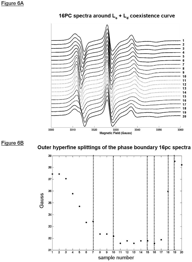
ESR spectra obtained from compositions along the coexistence curve reveal the expected compositional range for a critical point (CPR) and end tie-line (ETR) for the open coexistence curve configuration of the Lo + Ld coexistence region of SPM/DOPC/Chol. A) Stack plot of the 16PC ESR spectra on the coexistence curve showing the Lo spectra (solid lines), Ld spectra (dotted lines), and the CPR and ETR spectra (dashed lines). The low-field and high-field regions flanking the central peak in spectra 16, 17, and 18 show visually the appearance of gel-phase spectral components. B) Plot of the outer hyperfine splitting with sample number along the coexistence curve showing the CPR and ETR (between the dotted lines) having different profiles.
In summary, based on the analysis of the coexistence curve spectra, we estimate that a critical point lies somewhere between the compositions of point 7 (ξS = 0.217, ξD = 0.463, ξC = 0.320) and point 10 (ξS = 0.163, ξD = 0.697, ξC = 0.140), which we call the critical point region (CPR). Also, we estimate a three-phase coexistence boundary with vertex lying between point 15 (ξS = 0.524, ξD = 0.343, ξC = 0.133) and 16 (ξS = 0.570, ξD = 0.259, ξC = 0.171), and another vertex lying between point 18 (ξS = 0.632, ξD = 0.107, ξC = 0.261) and 19 (ξS = 0.634, ξD = 0.042, ξC = 0.324). Also, we concluded that samples 16 thru 18 were within the three-phase region. Therefore, for clarity of exposition, the transition region for the two vertices (points 15 thru 16 and points 18 thru 19) are called the end tie-line regions (ETR).
B. Performance of the tie-line field method on synthetic data sets
Before analyzing the actual experiments, we first performed tests of the method on synthetic data sets. A synthetic data set was generated by linearly combining the coexistence curve spectra for each composition in the coexistence region using an arbitrarily chosen critical point, end tie-line, value of c in Eqn 7 (to specify the TLF) and arbitrary coefficients in Eqn 14 and 15 (to specify the Kp function). The interior reflective Newton method with conjugate gradients (built-in Matlab function “lsqnonlin”) and the constrained simplex search method (“fminsearchcon” written by John D'Errico, woodchips@rochester.rr.com, released 12/16/06 and obtained from Matlab Central) were compared with data sets that had essentially no noise (s/n ∼ 3000) or were very noisy (s/n ∼ 70) to determine their effectiveness for fitting. It should be emphasized, however, that our experimental results are best approximated by the s/n ∼ 3000 case. The fitting was started from 10 random starting points, and true convergence to the global minimum was determined if the set of parameters obtained was within 5% of the true minimum.
The simplex search method outperformed the Newton search method in locating the global minimum for the very low-noise data sets; however, the simplex search had about four times as many function calls (data not shown). Both did equally poorly with the very noisy data. The ruled surface field with an open boundary configuration has six adjustable parameters (3 for the location of the critical point/end tie-line points, 1 for the tie-line field function, and 2 for the Kp function). In the low noise case, good convergence was obtained to the true values, but some trials yielded nearby local minima, differing slightly in the values of the parameters, but virtually the same TLF. We found this feature was closely associated with the initial (or seed) choice of the critical point and end tie-line boundary parameters.
Since we found that convergence of a fit to the true global minimum strongly depended on thoroughly searching the critical point and end tie-line boundary parameters, the procedure we used to stably analyze the real data set was to do a grid search over these parameters. The critical point search range was bounded by samples 7 and 10, and the grid interval was chosen as the boundary parameters of the intervening points. The end tie-line search range was bounded by samples 15/16 and 18/19, but no smaller interval was specified since these points were so close together and within the region of good convergence to a minimum. Therefore, at each point of the grid the boundary parameters of the critical point and end points of the end tie-line were fixed and the remaining search parameters were varied under the simplex search algorithm. After the minimum over all the grid points was found, a further simplex search was done within the restricted ranges for the critical point and the end tie-line to find the global minimum.
C. The best-fit ruled surface tie-line field
For the expected CPR and ETR (Figure 2A), the best-fit ruled surface parameters (χ2 = 34.38) and their errors are shown in Table 1. The uncertainty or errors in the parameters of the ruled surface TLF was determined by a Monte Carlo simulation (33), which proceeded as follows. During each iteration of the simulation, a synthetic data set was generated by adding normally distributed noise, with a variance taken from the spectral baseline, to the best-fit predicted spectra (SP) for each coexistence composition and uniformly distributed noise of 2% was added to the coexistence compositions themselves, then this synthetic data set is fit the same way as the real data set. The standard deviation of the distribution of the difference between the best-fit parameter from the synthetic data sets and the best-fit parameter from the real data set was the error estimate for that parameter. Since the ruled surface TLF parameters are highly coupled and interdependent, the sources of their uncertainty are difficult to diagnose. However, the lower the uncertainty the more confident we are in the value of the parameter and the more important the parameter is to getting the best-fit to the data. Therefore, the boundary parameters for the location of the critical point and end tie-line are the most important (i.e. the lowest uncertainty) in determining the best-fit to the ESR data (Table 1). The errors for these boundary parameters are close to the estimated variability of the data compositions (2%). The best-fit ruled surface tie-line field is shown in Figure 7A. The slopes of the tie-lines through the experimental coexistence compositions (Figure 7B) were calculated numerically. The slope of the end tie-line (u = 1) is 40°. The profile exhibited a maximum at u = 0.65 with a slope of 52.8°. This Lo boundary parameter corresponds to the tie-line that connects a Lo phase with composition, ξS = 0.401, ξD = 0.145, ξC = 0.454, having one of the highest concentrations of cholesterol, to an Ld phase with composition, ξS = 0.350, ξD = 0.595, ξC = 0.055, having one of the lowest concentrations of cholesterol. In addition, the slope for the lowest Lo boundary parameter for an experimental coexistence composition (u = 0.24) is 47.0°. As u approaches zero the tie-line slopes approach the slope of the tangent line to the critical point, as they should geometrically. However, the numerical calculation of the tie-line slopes near the critical point is unreliable because of the lack of sufficient data near the critical point, as well as the restrictions the tie-line field function imposes on the tie-line slopes as the critical point is approached. A more sophisticated tie-line field function that takes into account the slope of the tangent lines to the boundary approaching a critical point would be an improvement. A previously determined tie-line in this system from the TTL method was found to have a slope of 65° ± 5° (2). From the uncertainty in the tie-line field function parameter (“c” in Table 1), the error in the slope of a similar tie-line of the ruled surface tie-line field is 50° ± 5°. These results do not agree exactly, but, since the TTL and TLF methods are fundamentally different (e.g. the TTL method does not have the non-crossing constraint with respect to other tie-lines), we expect minor deviations. For all values of u, and thus all tie-lines, the Kp was greater than unity (Figure 7C), showing that 16PC preferentially partitions into the Lo phase. A Kp slightly greater than unity value (Kp = 1.1 ± 0.5) was found previously for the tie-line determined by the TTL method within this lipid system (2). This compares favorably to a similar tie-line in the ruled surface TLF with Kp = 1.6 ± 0.5 (where the uncertainty in Kp has been estimated from those of “a” and “b” in Table 1).
Table 1.
The parameters and their uncertainties (σ) of the best-fit ruled surface TLF for the open boundary configuration of the Lo + Ld coexistence region of the SPM/DOPC/Cholesterol lipid system.†
| Parameter | Critical point* | End tie-line vertex 1* | End tie-line vertex 2* | Tie-line field parameter (c) |
Kp parameter (a) |
Kp parameter (b) |
|---|---|---|---|---|---|---|
| value | 0.346 | 0.697 | 0.856 | 2.30 | 4.26 | −3.87 |
| σ | ±0.010 (2.9%) |
±0.016 (2.3%) |
±0.012 (1.3%) |
±0.43 (18.8%) |
±0.27 (6.3%) |
±0.36 (9.3%) |
The uncertainties were estimated by a Monte Carlo simulation. The number of Monte Carlo iterations was 100. To generate the synthetic data sets for the simulation, noise was added to the coexistence spectra and compositions but not to spectra and compositions on the coexistence curve.
These give the value of b, defined in Figure 4B, which gives the location on the coexistence curve.
Figure 7.
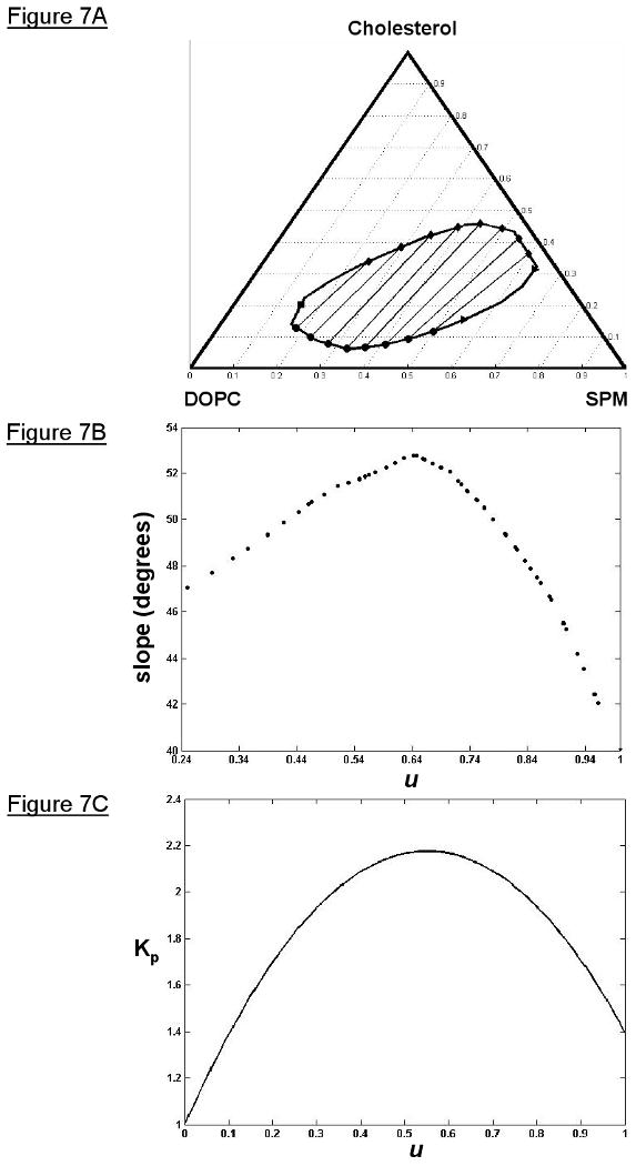
The ruled surface TLF best fit to the ESR data for the open boundary configuration of the Lo + Ld coexistence region of the SPM/DOPC/Chol lipid system with the expected CPR and ETR. A) A plot showing some tie-lines from the TLF, the critical point (square), end-points of the end tie-line (triangles), Lo phase compositions (diamonds), and Ld phase compositions (dots). B) The slope profile of the TLF showing a maximum slope of 52.8° and an end tie-line with a slope of 40°. C) The Kp function of the TLF showing a maximum Kp of 2.17 and a Kp of 1.40 at the end tie-line (u = 1); a Kp > 1 favors the Lo phase.
We have also considered two simpler models for a TLF that have been discussed previously (35). The simplest is, of course, one of parallel tie-lines. This case is easily implemented using our methodology. It is however too restrictive for a realistic multi-component system, (e.g. it requires the tangent to the critical point and the end tie-line, for an open system, to be parallel). Nevertheless, our result, using this approach, yields a parallel TLF with a slope of 33° from our data. The second approach is that of a “common vertex”. This refers to an intersection point formed by the intersection of the tangent to the critical point and the end tie-line. It is assumed that all tie-lines intersect this common vertex. We note that there are numerous experimental phase diagrams for many different systems which show TLF's that seem to conform to this configuration (35). Our analysis of this approach yielded tie-line slopes varying monotonically from 52° (for u = 0) to 41° (for u = 1). This is comparable to the range observed for the ruled surface (cf. Figure 7). Also we find the Kp varying from unity to a maximum of 2.1 (occurring at u ∼ 0.6), corresponding closely to the ruled surface result. However, we regard the ruled surface TLF approach as the more general one, which does not require the simplifying constraints of the parallel and common vertex models. Also, in a comparison of the three models, the ruled surface TLF gave the best fit statistically to the ESR data despite having more fitting parameters (results not shown).
V. Discussion
A. Conclusions from this study
The work presented in this paper provides several important conclusions. The TLF method provides a general way to experimentally determine tie-lines in any lipid system efficiently and with little or no constraint on the type of data. Furthermore, the ruled surface parameterization of tie-line fields allows a data fitting procedure to be formulated and solved using standard algorithms. This formulation also highlights the importance of the probe partition coefficient as the mediator between the TLF and the data. In the application of the TLF method to the Lo + Ld coexistence region of the SPM/DOPC/Chol lipid system, the determined TLF conformed to previous information on this lipid system, and it offers a path for further research in studying phase behavior.
Analysis of cw-ESR spectra from an appropriate spin-labeled probe can be used to determine phase transition regions containing critical points and end tie-lines bordering three-phase triangles in ternary lipid mixtures. The 16PC spectra from compositions along the Lo + Ld coexistence curve of the SPM/DOPC/Chol lipid system (Figure 6A) show clear transition regions from Lo phases to Ld phases, and this enables us to distinguish these regions as transiting through a critical point or a three-phase triangle. The spectra around the critical point exhibit smooth spectral changes, while spectra through the three-phase triangle exhibit gel-phase spectral components and abrupt spectral changes. Although the cw-ESR spectra from 16PC can only give a range of compositions, constraining the possible critical point and end tie-line locations greatly improves convergence to the global minimum because of their importance in the fitting procedure. Additional cw-ESR spectra from other probes or data from techniques with better resolution of components, such as 2D-ELDOR (10) may be sufficient to narrow the phase transition regions (i.e. CPR and ETR).
However, since we found that the critical point location is determined in the fitting to high precision, the TLF method provides a way, in principle, to determine very precisely the location of the critical point. We do not conclude that we precisely located the critical point for the Lo + Ld region of SPM/DOPC/Chol because of correlation in its fitting with the parameters for the tie-line field function and partition coefficient function, which have substantially greater uncertainty. Therefore, reduction of confidence intervals for these parameters, through higher quality data (e.g. 2D-ELDOR) and/or better tie-line field and partition coefficient functions, will improve the confidence of the exact location of the critical point.
B. Comparison of the TLF method to other experimental methods
There have been two other experimental methods to determine tie-lines in ternary lipid systems, the TTL method (1) and the method of Veatch et al (19). The main difference between them and the TLF method, as we previously noted, is that the latter determines all tie-lines through a coexistence region whereas the other methods determine one tie-line at a time, thereby generating a “coarse-grained” TLF. A disadvantage of determining a TLF one tie-line at a time is the non-trivial way of constraining the tie-lines to not intersect; whereas, in the TLF method, this constraint is implicit in the ruled surface parameterization. In addition, as we have already shown, the TLF method is more efficient in its data requirements. The main similarity of all three methods is the application of the linear superposition model to magnetic resonance spectra. Both the TLF and TTL method were used to analyze ESR spectra and the Veatch et al method to analyze NMR spectra; however, each of these methods should be equally applicable to studies using ESR or NMR data. That is, the data analysis employing the linear superposition model and the lever rule involve common aspects independent of the source of the spectra. Therefore, a comparison of the TLF method with the other tie-line determination methods, independent of data type, is appropriate.
As already mentioned, the TLF method and the TTL method share a similar fit criterion; however, they differ in the manner of searching for the tie-lines: either one at a time as in the TTL method, or the field as in the TLF method. Although both methods use compositions and spectra from the coexistence curve, the TTL method directly searches for a tie-line by varying the slope of trial tie-lines from a common point on the coexistence curve, with each trial tie-line containing a linear arrangement of sample compositions through the coexistence region. The TLF method searches the tie-line fields by varying the parameters for the ruled surface parameterization. As a result, in the TTL method, the slopes of the trial tie-lines are naturally constrained with respect to each other, but within the “coarse-grained” TLF, the slopes of the best-fit trial tie-lines are essentially unconstrained with respect to each other. An advantage of the direct search for a tie-line in the TTL method is that many samples of data along a trial tie-line offer a statistically better estimation of the Kp and its standard deviation for that trial tie-line. This estimation of Kp variability is needed when comparing other trial tie-lines because of the requirement of constant Kp along tie-lines. The disadvantage of the TTL method is the amount of work needed to determine a “coarse-grained” TLF. For example, we used a total of 71 samples for the TLF method in this work and 77 samples to determine one tie-line in the same lipid system using the TTL method (2).
The Veatch et al method is a much different one from the TLF method. Their method is an attempt to generalize a well-known NMR method for determining phase boundaries in binary systems (36, 37) to use for determining tie-lines (and phase boundaries) in ternary systems. The NMR method for determining phase boundaries in binary systems (where the tie-lines are immediately known) consists of two basic steps: 1) Spectral subtraction of two spectra from two coexistence compositions (A and B) to get the basis (i.e. tie-line end-point) spectra and the fractions of total deuterated (D) lipid probe and for each coexistence spectra (i = A,B). This method relies on the ability to clearly distinguish the spectra for each phase. The basis spectra are determined by visual inspection using the concept of a “reference” spectrum for each phase. 2) Then these values of and the overall mole fractions of DPPC and Cholesterol in these samples can be used with the conservation of matter equations (Eqn. 3 including associated definitions, but for binary systems) to obtain the phase boundary compositions given by and .
The Veatch et al method requires “reference” spectra representing just the Lo phase and just the Ld phase. Then they obtain spectra within the two-phase region. But here they obtain a spectrum for a single composition A and a range of B compositions along a line within the coexistence region. By means of spectral subtraction of the A spectrum from each of the B spectra they obtain a series of “trial” Lo and Ld spectra, which are then compared with the reference spectra. The best estimate of the tie-line is taken as the line connecting the point A with that composition of B yielding the best agreement between the spectral subtraction results and the reference spectra in a least squares sense. Only one (or a few) reference spectra are taken in each phase. The assumption is made that there is little change with composition in the NMR spectrum taken within a single phase, and whatever spectral change occurs may be approximately corrected by small changes in ordering requiring only a small rescaling of the spectral frequency (x) axis. This is done as part of the least square fitting. Once the best tie-line slope is determined, the end-points of the tie-line are found by substituting and for the fraction of Lo and Ld phase into the conservation of matter equations (Eqn 3), rewritten as a homogeneous system of equations, and solving the system for the phase boundary (end-point) compositions. The fractions of total deuterated lipid probe in each phase, and , are determined from the spectral subtraction in step one. However, the above equations for the fractions of phase only apply to binary systems because they are derived from the binary lever rule; their substitution into the conservation of matter equations for the ternary system decouples the problem into the projections on the binary axes. But these equations are not the same as for the ternary system, because the ternary lever rule is not conserved under this projection. The lever rule for ternary systems is given in Eqn 4 and is a function of the mole fractions of two components (unlike binary systems); therefore, the fraction of one other component, either DOPC or Cholesterol, in each phase needs to be determined by a similar spectral subtraction procedure to solve for the phase boundaries.
Taking into account the inherent differences between ESR and NMR spectra, the TLF method has no disadvantages over the other methods, since it can be applied to either data with little or no modification. Therefore, the issue with the type of data has more to do with quality than methodology. In an ESR experiment, the spin-probe is added to the lipid system in low concentrations, whereas, in an NMR experiment, the deuterated lipid probe is a component of the system. In applying the TLF method to NMR spectra, this probe property would allow replacing the Kp(u) function with , which can be calculated from the ruled surface parameterization of the TLF, is dependent on the coexistence curve, and satisfies the boundary conditions for both the open and closed coexistence curve configurations. However, a disadvantage of an NMR experiment would be the great expense in making the many deuterated samples required for the TLF method. In addition, two ideal properties of any spectral data to be fit with the TLF method are to have significantly different lineshapes for different phases and to change appreciably with variable composition within one phase. Because both ESR and NMR lipid probes are sensitive to the ordering of the lipid acyl chains, both types of spectra typically have much different lineshapes in different phases; however, since an ESR probe is more sensitive to lipid dynamics, the ESR spectra tend to change more noticeably along the coexistence curve with changing composition (1, 10, this study). In the DPPC/Chol binary system, studies employing 2H-NMR (37, 38) observed only small differences in the Ld and Lo spectra vs. temperature and composition, thus rendering a spectral subtraction analysis for phase boundaries very difficult. One proposed reason for the spectral similarity is exchange averaging over small liquid phase domains within the NMR timescale (37); however, in the ternary systems with DOPC, the Lo + Ld coexistence region exhibits large phase domains (12). Another reason is the reduced resolution arising from the superposition of 2H NMR spectra from all positions along the acyl chains (38).
C. Tie-lines and theoretical interpretations
The general consensus is that the phase behavior of ternary lipid systems containing a gel-forming saturated phospholipid, an Ld-forming unsaturated phospholipid, and cholesterol would be similar. In fact, the phase diagrams of the DPPC/DOPC/Chol, DSPC/DOPC/Chol, and SPM/DOPC/Chol lipid systems do contain similar two-phase coexistence regions along with a three-phase triangle. However, the steeper slopes of the tie-lines for the Lo + Ld coexistence region of the SPM/DOPC/Chol mixture obtained from the TTL method (2) and the TLF method (this work) contrast with the shallower slopes of the tie-lines for the Lo + Ld coexistence region of the DPPC/DOPC/Chol mixture obtained using the Veatch et al method (20). The TLF of the DPPC system (20) was assumed to be parallel because the slope of the determined tie-line was roughly parallel to the end tie-line of the neighboring three-phase triangle. The TLF of the SPM system is not parallel (Figure 7A, B), but has the smallest slope at the end tie-line with increasing slopes connecting the Lo phases with the highest amounts of cholesterol to the Ld phases with the lowest amounts of cholesterol and then decreasing slopes approaching the critical point.
The slopes of tie-lines are significant because they show the difference in lipid mole fractions between each phase, which reflects the favorable or unfavorable interactions between the lipids. For example, a 60° slope implies that the SPM (or DPPC) mole fraction is constant in the two phases with the larger differences in the mole fractions of DOPC and cholesterol, suggesting that the energetic repulsion between DOPC and cholesterol drives the Lo and Ld phase separation. This is reasonable because of the predicted poor packing between the rigid ring structure of cholesterol and an unsaturated acyl chain, especially with the double bond of DOPC in the middle of the chain. Shallower tie-line slopes show less of a difference in the cholesterol mole fraction and a greater difference in the SPM (or DPPC) and DOPC mole fraction between the Ld and Lo phases, suggesting the energetic interaction driving phase separation is the attraction of well-aligned saturated chains for each other.
Elliot et al (22) proposed a statistical model using mean-field theory that takes into account lipid packing with a tendency to align the chains with the bilayer normal. This tendency is a result of the long-range attraction between lipids due to the hydrophobic effect. In this model, cholesterol interacts equally well with the bonds of unsaturated or saturated acyl chains, but cholesterol is more repulsed by unsaturated chains overall because of poor packing. Their model predicted tie-lines with approximately 60° slopes for the Lo + Ld coexistence region of a saturated/unsaturated/cholesterol lipid system (39).
The Elliot et al model contrasts with McConnell's condensed complex model (21). In McConnell's regular solution theory, saturated lipids and cholesterol chemically react forming complexes which can interact as a unit with the unsaturated lipid and unbound saturated lipid and cholesterol. This model emphasizes a stronger attraction of cholesterol to saturated chains instead of unsaturated chains over a background tendency to mix uniformly as required by the thermodynamic entropy of mixing. A calculated DPPC/DOPC/Chol phase diagram with the condensed complex model shows tie-lines with slopes of approximately 30° for the Lo + Ld region (21). Indeed, the phase diagrams of both the DSPC/DOPC/Chol and DPPC/DOPC/Chol systems show the end tie-line of the Lo + Ld region with a shallow slope between 10° and 30°, with the determined tie-line in the DPPC system also having this slope (20).
The TLF of the SPM/DOPC/Chol system also has a shallow slope for the end tie-line but steeper slopes with increasing concentrations of DOPC. This result suggests that at higher saturated lipid amounts near the three-phase triangle the Lo and Ld phase separation is driven by the attraction of chain alignment, whereas with increasing amounts of unsaturated lipid the tie-lines bend to steeper slopes, reflecting the greater contribution of the packing repulsion between unsaturated chains and cholesterol to the free energy. More experimentally determined tie-line fields of ternary lipids systems will be needed to resolve whether there is any discrepancy of the steeper slopes in the SPM system than the saturated glycerophospholipid system.
Acknowledgments
We are grateful for many helpful discussions at the early stages of this work with Professors Gerald Feigenson and Benjamin Widom and to a critical reading of the manuscript by Professor Jozef K. Moscicki. This work was supported by NIH grants R01-ER03150 and P41-RR016292.
Appendix A: Definitions of Symbols and Abbreviations
Subscripts: S = Sphingomyelin, D = DOPC, C = Cholesterol
Superscripts: o = Lo phase, d = Ld phase
i = S, D, or C and j = o or d
ξi = = total mole fraction of component i (cf. Eqn 1)
ξ = vector of mole fractions ξi for the whole sample (cf. Eqn 1)
ψ = coordinate transform of ξ (cf. Eqn 2)
= mole fraction of component i in the jth phase (cf. Eqn 3)
ξj = vector of mole fractions for the jth phase (cf. Eqn 3)
ψj = coordinate transform of ξj (cf. Eqn 4)
= number of moles of component i in the jth phase
Ni = = total number of moles of component i
Nj = = total number of moles of the jth phase
N = = total number of moles
φj = = mole fraction of the jth phase (cf. Eqns 3, 4)
u = chord-length parameter for Lo phase boundary; specifies tie-line (cf. Eqn 6)
v(u) = chord-length parameter for Ld phase boundary (cf. Eqn 6)
S = spectrum of the whole sample (cf. Eqn 8)
Sj = spectrum of the jth phase (cf. Eqn 8)
fj = = fraction of total probe in the jth phase (cf. Eqn 8)
Kp(u) = predicted partition coefficient for parameter u (cf. Eqns 14, 15)
= reduced (unweighted) Chi-square for the kth trial tie-line (cf. Eqn 16)
= standard deviation of Kp for the kth trial tie-line (cf. Eqn 16)
(χ2)k = weighted Chi-square for the kth trial tie-line (cf. Eqn 16)
TTL = trial tie-line, TLF = tie-line field, HTLF = hypothetical tie-line field, CPR = critical point region, ETR = end tie-line region
References
- 1.Chiang YW, Zhao J, Wu J, Shimoyama Y, Freed JH, Feigenson GW. Biochim Biophys Acta. 2005;1668:99. doi: 10.1016/j.bbamem.2004.11.010. [DOI] [PubMed] [Google Scholar]
- 2.Swamy MJ, Ciani L, Ge M, Smith AK, Holowka D, Baird B, Freed JH. Biophys J. 2006;90:4452. doi: 10.1529/biophysj.105.070839. [DOI] [PMC free article] [PubMed] [Google Scholar]
- 3.Smith AK, Buboltz JT, Spink CH, Feigenson GW. Biophys J. 2003;84:372a. [Google Scholar]
- 4.Laughlin RG. Tetrahedron. 1997;53:9997. [Google Scholar]
- 5.Sengers JL. How fluids unmix Discoveries by the School of Van der Waals and Kamerlingh Onnes. Royal Netherlands Academy of Arts and Sciences; Amsterdam: 2002. [Google Scholar]
- 6.Feigenson GW. Annu Rev Biophys Biomol Struct. 2007;36:63. doi: 10.1146/annurev.biophys.36.040306.132721. [DOI] [PMC free article] [PubMed] [Google Scholar]
- 7.London E. Biochim Biophys Acta. 2005;1746:203. doi: 10.1016/j.bbamcr.2005.09.002. [DOI] [PubMed] [Google Scholar]
- 8.Edidin M. Annu Rev Biophys Biomol Struct. 2003;32:257. doi: 10.1146/annurev.biophys.32.110601.142439. [DOI] [PubMed] [Google Scholar]
- 9.Simons K, Winchil LCV. Annu Rev Biophys Biomol Struct. 2004;33:269. doi: 10.1146/annurev.biophys.32.110601.141803. [DOI] [PubMed] [Google Scholar]
- 10.Chiang YW, Costa-Filho AJ, Freed JH. J Phys Chem B. 2007;111:11260. doi: 10.1021/jp0732110. [DOI] [PubMed] [Google Scholar]
- 11.Zhao J, Wu j, Heberle FA, Mills TT, Klawitter P, Huang G, Costanza G, Feigenson GW. Biochim Biophys Acta. 2007;1768:2764. doi: 10.1016/j.bbamem.2007.07.008. [DOI] [PMC free article] [PubMed] [Google Scholar]
- 12.Veatch SL, Polozov IV, Gawrisch K, Keller SL. Biophys J. 2004;86:2910. doi: 10.1016/S0006-3495(04)74342-8. [DOI] [PMC free article] [PubMed] [Google Scholar]
- 13.Kahya N, Scherfeld D, Bacia K, Schwille P. J Struct Biol. 2004;147:77. doi: 10.1016/j.jsb.2003.09.021. [DOI] [PubMed] [Google Scholar]
- 14.Veatch SL, Keller SL. Phys Rev Lett. 2005;94:148101. doi: 10.1103/PhysRevLett.94.148101. [DOI] [PubMed] [Google Scholar]
- 15.Feigenson GW, Buboltz JT. Biophys J. 2001;80:2775. doi: 10.1016/S0006-3495(01)76245-5. [DOI] [PMC free article] [PubMed] [Google Scholar]
- 16.de Almeida RFM, Fedorov A, Prieto M. Biophys J. 2003;85:2406. doi: 10.1016/s0006-3495(03)74664-5. [DOI] [PMC free article] [PubMed] [Google Scholar]
- 17.Heberle FA, Buboltz JT, Stringer D, Feigenson GW. Biochim Biophys Acta. 2005;1746:186. doi: 10.1016/j.bbamcr.2005.05.008. [DOI] [PMC free article] [PubMed] [Google Scholar]
- 18.Buboltz JT. Physical Review E. 2007;76:021903. doi: 10.1103/PhysRevE.76.021903. [DOI] [PubMed] [Google Scholar]
- 19.Veatch SL, Gawrisch K, Keller SL. Biophys J. 2006;90:4428. doi: 10.1529/biophysj.105.080283. [DOI] [PMC free article] [PubMed] [Google Scholar]
- 20.Veatch SL, Soubias O, Keller SL, Gawrisch K. P N A S. 2007;104:17650. doi: 10.1073/pnas.0703513104. [DOI] [PMC free article] [PubMed] [Google Scholar]
- 21.McConnell HM. Biophys J. 2005;88:L23. doi: 10.1529/biophysj.104.058834. [DOI] [PMC free article] [PubMed] [Google Scholar]
- 22.Elliot R, Katsov K, Schick M. J Chem Phys. 2005;122:044904. doi: 10.1063/1.1836753. [DOI] [PubMed] [Google Scholar]
- 23.Tedrow PM, Lee DM. Physical Review. 1969;181:399. [Google Scholar]
- 24.Bahari Z, Rivet J, Legendre B, Dugue J. Journal of Alloys and Compounds. 1999;289:99. [Google Scholar]
- 25.Kundrat DM, Elliott JF. Metallurgical Transactions A. 1986;17A:1461. [Google Scholar]
- 26.Orr FM, Jr, Dindoruk B, Johns RT. Ind Eng Chem Eng. 1995;34:2661. [Google Scholar]
- 27.Buboltz JT, Feigenson GW. Biochim Biophys Acta. 1999;1417:232. doi: 10.1016/s0005-2736(99)00006-1. [DOI] [PubMed] [Google Scholar]
- 28.Huang J, Buboltz JT, Feigenson GW. Biochim Biophys Acta. 1999;1417:89. doi: 10.1016/s0005-2736(98)00260-0. [DOI] [PubMed] [Google Scholar]
- 29.Palatnik LS, Landau AI. Phase Equilibria in Multicomponent Systems. Holt, Rinehart and Winston, Inc.; New York: 1964. [Google Scholar]
- 30.Gordon P. Principles of Phase Diagrams in Materials Systems. McGraw-Hill Book Company; New York: 1968. [Google Scholar]
- 31.Gray A, Abbena E, Salamon S. Modern Differential Geometry of Curves and Surfaces with Mathematica. 3rd. Ch 14. Boca Raton, FL: CRC Press; 2006. Ruled Surfaces; p. 432. [Google Scholar]
- 32.Wang CCL, Tang K. Journal of Computing and Information Science and Engineering. 2005;5:291. [Google Scholar]
- 33.Schneider DJ, Freed JH. Biological Magnetic Resonance. 1989;8:1. [Google Scholar]
- 34.Press WH, Flannery BP, Teukolsky SA, Vetterling WT. Numerical Recipes in C: The Art of Scientific Computing. 2nd. Cambridge University Press; London: 1992. [Google Scholar]
- 35.Bachman I. J Phys Chem. 1940;44:446. [Google Scholar]
- 36.Hsueh YW, Gilbert K, Trandum C, Zuckermann M, Thewalt J. Biophysical Journal. 2005;88:1799. doi: 10.1529/biophysj.104.051375. [DOI] [PMC free article] [PubMed] [Google Scholar]
- 37.Vist MR, Davis JH. Biochemistry. 1990;29:451. doi: 10.1021/bi00454a021. [DOI] [PubMed] [Google Scholar]
- 38.Huang TH, Lee CWB, Das Gupta SK, Blume A, Griffin RG. Biochemistry. 1993;32:13277. doi: 10.1021/bi00211a041. [DOI] [PubMed] [Google Scholar]
- 39.Elliot R, Szleifer I, Schick M. Physical Review Letters. 2006;96:098101. doi: 10.1103/PhysRevLett.96.098101. [DOI] [PubMed] [Google Scholar]