Analysis of MALDI FT-ICR Mass Spectrometry Data: a Time Series Approach

Abstract

Matrix-assisted laser desorption/ionization Fourier transform ion cyclotron resonance mass spectrometry is a technique for high mass-resolution analysis of substances that is rapidly gaining popularity as an analytic tool. Extracting signal from the background noise, however, poses significant challenges. In this article, we model the noise part of a spectrum as an autoregressive, moving average (ARMA) time series with innovations given by a generalized gamma distribution with varying scale parameter but constant shape parameter and exponent. This enables us to classify peaks found in actual spectra as either noise or signal using a reasonable criterion that outperforms a standard threshold criterion.

1 Introduction

Matrix-assisted laser desorption/ionization Fourier transform ion cyclotron resonance mass spectrometry (MALDI FT-ICR MS) is a technique for high mass-resolution analysis of substances that is rapidly gaining popularity as an analytic tool in proteomics. Typically in MALDI FT-ICR MS, a sample (the analyte) is mixed with a chemical that absorbs light at the wavelength of the laser (the matrix ) in a solution of organic solvent and water. The resulting solution is then spotted on a MALDI plate and the solvent is allowed to evaporate, leaving behind the matrix and the analyte. A laser is fired at the MALDI plate and is absorbed by the matrix. The matrix becomes ionized and transfers charge to the analyte, creating the ions of interest (with fewer fragments than would be created by direct ablation of the analyte with a laser). The ions are guided with a quadrupole ion guide into the ICR cell where the ions cyclotron in a magnetic field. While in the cell, the ions are excited and ion cyclotron frequencies are measured. The angular velocity, and therefore the frequency, of a charged particle is determined solely by its mass-to-charge ratio. Using Fourier analysis, the frequencies can be resolved into a sum of pure sinusoidal curves with given frequencies and amplitudes. The frequencies correspond to the mass-to-charge ratios and the amplitudes correspond to the concentrations of the compounds in the analyte. FT-ICR MS is known for high mass resolution, with separation thresholds on the order of 10⁻³ Daltons (Da) or better [1, 2].

The spectra analyzed in this article were recorded on an external source MALDI FT-ICR instrument (HiResMALDI, IonSpec Corporation, Irvine, CA) equipped with a 7.0 T superconducting magnet and a pulsed Nd:YAG laser 355 nm. In addition to hundreds of spectra generated as described above for a cancer study [3] using human blood serum as the analyte, we generated 56 spectra using neither analyte nor matrix. We will refer to the latter category of spectra as “noise spectra” and use them in Sections 2 and 3 to develop our model, then apply the model to a spectrum with known contents in Section 4.

We find that an autoregressive, moving average (ARMA) time series with innovations given by a generalized gamma distribution can closely model the properties of the noise spectra, and that this representation is useful for accurately identifying real substances in spectra produced using analyte. The modeling assumptions developed in this article are implemented in the R package FTICRMS, available either from the Comprehensive R Archive Network (http://www.r-project.org/) or from the first author.

2 Methods

2.1 Description of data

A typical noise spectrum is shown in Figure 1 with frequency in kilohertz (kHz) plotted on the horizontal axis. (In the mass spectrometry literature, it is more usual to see m/z—the mass-to-charge ratio—on the horizontal axis, but the actual process of measurement uses equally-spaced frequencies, and the m/z values are computed using one of several non-linear transformations on the frequencies [4]. Thus, the spectrum pictured in Figure 1 is how it appears after the Fast Fourier Transform is applied to the measured data.) The thick spike at a frequency of roughly 40 kHz is actually two peaks at frequencies 41.21 kHz and 42.21 kHz which extend upward to intensities of approximately 222.7 and 95.4, respectively, and are apparently instrumental noise—they appear in all 56 noise spectra at roughly the same spots and have no isotope peaks. In the analysis that follows, we set the values of the spectra at frequencies corresponding to these two peaks to be missing.

Figure 1.

Typical Noise Spectrum. A MALDI FT-ICR spectrum produced without matrix or analyte. The spike extending off the top of the picture is actually two peaks at frequencies of 41.21 kHz and 42.21 kHz which extend upward to intensities of approximately 222.7 and 95.4, respectively.

2.2 Properties of noise spectra

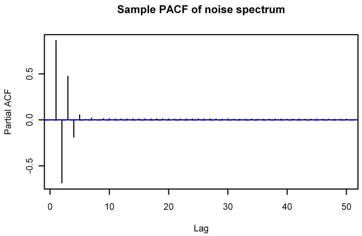
We start by considering two striking properties of the noise spectra. The first property is the special forms of the sample autocorrelation function (ACF) and sample partial autocorrelation function (PACF) of the noise spectra; Figure 2 displays the graphs of the sample ACF and sample PACF of the noise spectrum from Figure 1. Starting with lag 7, the sample ACF is nearly constant at roughly 0.0613. The sample PACF, on the other hand, oscillates between positive and negative values before decaying to a small positive value. As we show in Section 2.3, the sample ACF enables us to get information not only about the baseline but also about the coefficients to use in the ARMA representation of the spectrum. The sample PACF will be useful for evaluating the final ARMA model for accuracy.

Figure 2.

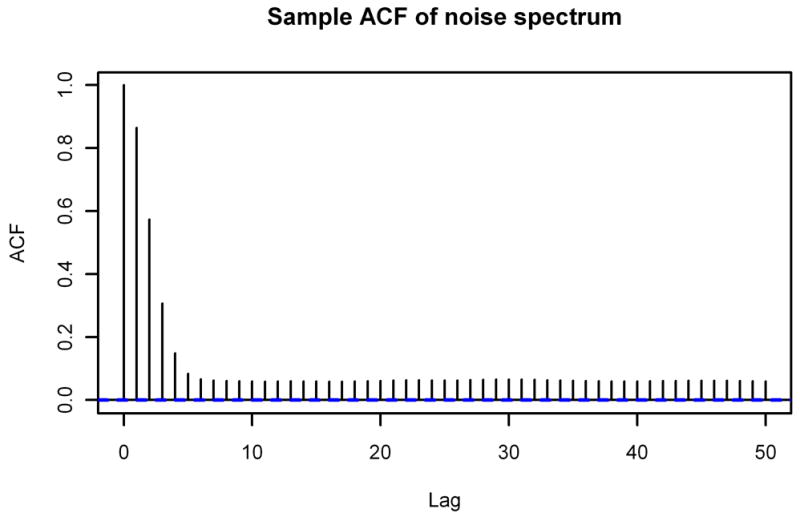
Sample ACF and Sample PACF of Typical Noise Spectrum. The sample autocorrelation function (top) and sample partial autocorrelation function (bottom) through lag 50 of the noise spectrum from Figure 1.

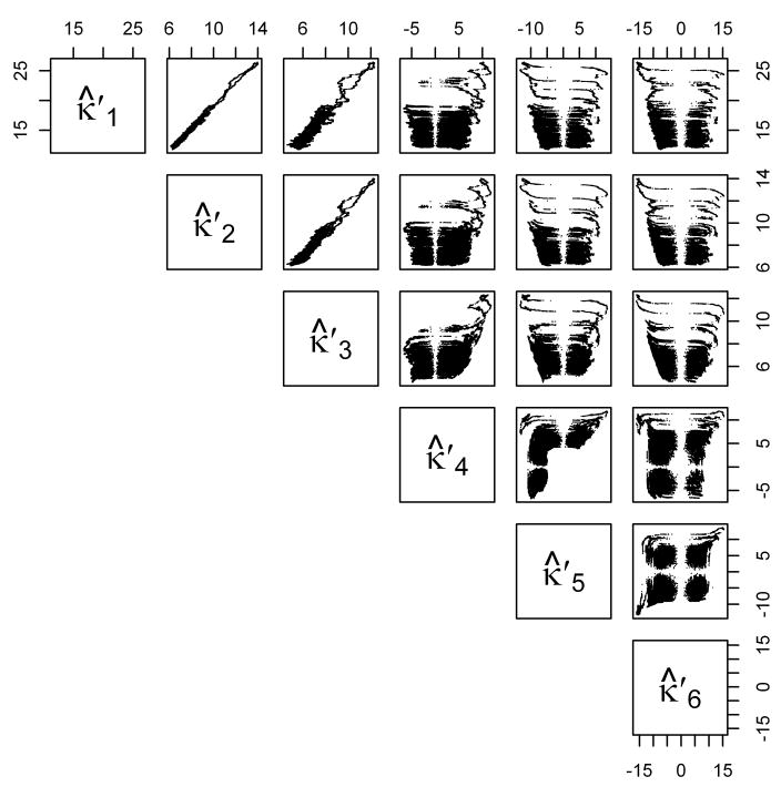
The second property comes from looking at the sample “homogenized” cumulants ${\widehat{\kappa }}_1^{\prime },{\widehat{\kappa }}_2^{\prime }$, … of the spectrum. (The sample homogenized cumulants of a set of data are related to the mean, variance, skewness, kurtosis, etc., of the data and will be defined precisely in Section 2.4, Equation (5).) Figure 3 displays scatterplots of the running sample homogenized cumulants (with bandwidth 4001 points—other bandwidths give similar plots) of the noise spectrum from Figure 1. It is clear that the first three sample homogenized cumulants have strong relationships. As we show in Section 2.4, this enables us to get information about the proper parameters to use in the generalized gamma distribution for the innovations in the ARMA representation of the spectrum.

Figure 3.

Sample Homogenized Cumulants of Typical Noise Spectrum. Running sample homogenized cumulants (bandwidth 4001 points) for the noise spectrum from Figure 1. See Section 2.4 for details.

2.3 Analysis of the ACF

The sample ACF r̂_k at lag k of a realization ${\{y_t\}}_{t=1}^n$ of a time series ${\{Y_t\}}_{t=1}^n$ is defined by

$${\widehat{r}}_k=\frac{{\sum }_{t=k+1}^n(y_t-\overline{y})(y_{t-k}-\overline{y})}{{\sum }_{t=1}^n{(y_t-\overline{y})}^2},$$ (1)

where ȳ is the sample mean. This is usually defined for stationary time series, in which (among other criteria) the means {μ_t} of the underlying random variables {Y_t} are assumed to be constant. However, estimating the underlying means for a noise spectrum by some method (running means, running medians, etc.) clearly shows that they are not constant.

Thus, suppose that $Y_t\sim ({\mu }_t,{\sigma }_t^2)$ with known means ${\{{\mu }_t\}}_{t=1}^n$ and suppose that the correlation between Y_t and Y_t−k is given by ρ̃_k (independent of t). Then, we have

$$\begin{array}{l}{\stackrel{\sim }{\rho }}_k=\frac{\mathbb{E}\{(Y_t-{\mu }_t)(Y_{t-k}-{\mu }_{t-k})\}}{\sqrt{\mathbb{E}\{{(Y_t-{\mu }_t)}^2\}}·\sqrt{\mathbb{E}\{{(Y_{t-k}-{\mu }_{t-k})}^2\}}}\\ {\stackrel{\sim }{\rho }}_k\sum _{t=1}^n{(y_t-{\mu }_t)}^2\approx \sum _{t=k+1}^n(y_t-{\mu }_t)(y_{t-k}-{\mu }_{t-k}),\end{array}$$ (2)

where is the expected value operator. We subtract the right-hand side of Equation (2) from the left and add the result to the numerator in Equation (1). This gives us

$${\widehat{r}}_k\approx \frac{{\sum }_{t=k+1}^n(y_t-\overline{y})(y_{t-k}-\overline{y})+{\stackrel{\sim }{\rho }}_k{\sum }_{t=1}^n{(y_t-{\mu }_t)}^2-{\sum }_{t=k+1}^n(y_t-{\mu }_t)(y_{t-k}-{\mu }_{t-k})}{{\sum }_{t=1}^n{(y_t-\overline{y})}^2}.$$ (3)

We can use Equation (3) to approximate r̂_k when the underlying correlations ρ̃_k are approximately zero. Write Y_t = μ_t + ε_t, where ε_t = 0; μ_t and ε_s are independent for all s, t; and k is large enough such that ε_tε_t−k = 0 but is small compared to n. We then get

$$\begin{array}{l}{\widehat{r}}_k\approx \frac{{\sum }_{t=k+1}^n(y_t-\overline{y})(y_{t-k}-\overline{y})}{{\sum }_{t=1}^n{(y_t-\overline{y})}^2}\\ \approx \frac{{\sum }_{t=k+1}^n({\mu }_t+{\epsilon }_t-\overline{\mu })({\mu }_{t-k}+{\epsilon }_{t-k}-\overline{\mu })}{{\sum }_{t=1}^n{(y_t-\overline{y})}^2}\\ \approx \frac{{\sum }_{t=k+1}^n({\mu }_t-\overline{\mu })({\mu }_{t-k}-\overline{\mu })+{\sum }_{t=k+1}^n{\epsilon }_t{\epsilon }_{t-k}}{{\sum }_{t=1}^n{(y_t-\overline{y})}^2}\\ {\widehat{r}}_k\approx \frac{{\rho }_{\mu }(k)·\text{Var}(\{{\mu }_t\})}{\text{Var}(\{y_t\})},\end{array}$$ (4)

where ρ_μ(k) is the autocorrelation of the means at lag k, which for small k should be close to 1 if the mean is slowly changing. Similar calculations show that Equation (4) also holds if Y_t = μ_t(1 + ε_t)—so the error is proportional to the mean—which will actually be the case for our spectra. In particular, for the noise spectrum pictured in Figure 1— using running means with bandwidth 4001 points to estimate {μ_t}—we get Var({μ_t}) ≈ 3.86, Var({y_t}) ≈ 62.0, and ρ_μ(k) > 0.999 for all k ≤ 100. These values give an estimate of r̂_k ≈ 0.0622, which closely matches the eventual value 0.0613 of the ACF in Figure 2.

Furthermore, we note that the sample ACF pictured in Figure 2 reaches the estimated value of 0.0622 for k ≥ 7 but is larger than that for k ≤ 6. That suggests that the underlying correlations ρ̃_k are nonzero for k ≤ 6 and zero for k ≥ 7. This, along with the rapidly decaying sample PACF, indicates that an MA(6) process would be a reasonable model for the spectrum. However, as we show in the next section, a general ARMA process fits the spectrum much better.

2.4 Analysis of the cumulants

The cumulants κ_n(X) of a random variable X are related to the coefficients of the Taylor expansion of log(e^itX) via

$$log(\mathbb{E}{e}^{\mathit{itX}})=\sum _{n=1}^{\infty }{\kappa }_n(X)·\frac{{(it)}^n}{n!}.$$

The most important property that cumulants have is that for independent random variables X and Y, we have κ_n(X + Y) = κ_n(X)+ κ_n(Y) for all n ≥ 1. (Contrast this with the central moments, where this property holds only for n = 1, 2, 3.) The first cumulant is equivariant under translation (i.e., κ₁(X + c) = κ₁(X)+ c for any constant c), and the higher-order cumulants are invariant under translation (i.e., κ_n(X + c) = κ_n(X) for n ≥ 2). In addition, the cumulants are homogeneous of degree n (i.e., κ_n(cX) = cⁿ · κ_n(X) for all n). Finally, we have κ₁(X) = X, κ₂(X) = Var(X), and κ₃(X) = {(X − X)³}, the mean and first two nonzero central moments of X. (This relationship does not hold for higher-order cumulants and central moments.)

For ease of presentation, we also introduce “homogenized cumulants” ${\kappa }_n^{\prime }(X)$ as

$${\kappa }_n^{\prime }(X)=\text{sign}\{{\kappa }_n(X)\}·\mid {\kappa }_n(X){\mid }^{1/n},$$ (5)

which are translation-equivariant for n = 1, translation-invariant for n ≥ 2, and homogeneous of degree 1 for all n. (It is these quantities, not the actual cumulants, that are plotted in Figure 3.)

For the remainder of this article, we will use capital letters to denote random variables and corresponding lower-case letters to denote realizations of those random variables. Thus, for example, the spectrum pictured in Figure 1 is {y_t} for the time series {Y_t}. The values of the sample cumulants and sample homogenized cumulants (estimated from data) will be denoted by κ̂_n and ${\widehat{\kappa }}_n^{\prime }$, respectively.

As Figure 3 shows, ${\widehat{\kappa }}_2^{\prime }(Y_t)/{\widehat{\kappa }}_1^{\prime }(Y_t),{\widehat{\kappa }}_3^{\prime }(Y_t)/{\widehat{\kappa }}_1^{\prime }(Y_t)$, and ${\widehat{\kappa }}_3^{\prime }(Y_t)/{\widehat{\kappa }}_2^{\prime }(Y_t)$ are all nearly constant across the entire spectrum. Let {Ỹ_t} be the de-trended series obtained from {Y_t} by dividing by the mean: Ỹ_t = Y_t/μ_t. Then {Ỹ_t} should have a constant mean of 1 and constant variance, so it would be a stationary time series if, in addition, the auto-correlations did not depend on t. We checked this assumption by estimating μ̂_t as a running mean with bandwidth 4001 points and considering the spectra given by $y_t^{\prime }=y_t/{\widehat{\mu }}_t$. We divided each of these into 486 groups of 2000 points. For each spectrum we then calculated first six lags of the sample ACF for each of the 486 groups of points (denoted by ρ̂) and compared the resulting values to the first six lags of the sample ACF of the whole spectrum (denoted by ρ). From a standard result in time series analysis (see, e.g., Shumway and Stoffer [5, Theorem A.7]), we know that ρ̂ ~ AN(ρ, W/n), where n is the length of the time series and the covariance matrix W is computable from the full ACF of the actual time series {Y_t}. Using the sample ACF of the entire spectrum {y_t} to estimate ρ and W, for each set of 2000 points we computed (ρ̂ − ρ)′(W/2000)⁻¹(ρ̂ − ρ), which under the null hypothesis of stationarity would be distributed as ${\chi }_6^2$. At the 0.05 level of significance, we find that on average 28/486 ≈ 0.058 of the sets of points have a significantly different sample ACF than the entire spectrum—very close to the number expected under the null hypothesis.

Thus, there is good evidence that the de-trended series {Ỹ_t} is, in fact, stationary. If {Ỹ_t} arises as a causal ARMA process, then we can write

$$\begin{array}{l}{\kappa }_n({\stackrel{\sim }{Y}}_t)={\kappa }_n\left(\sum _{k=0}^{\infty }{\psi }_k{X}_{t-k}\right)\\ =\sum _{k=0}^{\infty }{\psi }_k^n{\kappa }_n(X_{t-k})\\ =m_n{\kappa }_n(X_t)\\ {\kappa }_n^{\prime }({\stackrel{\sim }{Y}}_t)=\text{sign}(m_n)\mid m_n{\mid }^{1/n}{\kappa }_n^{\prime }(X_t),\end{array}$$

where $m_n\equiv {\sum }_{k=0}^{\infty }{\psi }_k^n$. In particular, the innovations {X_t} will also have proportional cumulants.

Thus, we should look for a distribution for the innovations for which the second and third cumulants remain proportional to the mean as the mean varies. One such distribution is given by the generalized gamma distribution with exponent α, shape parameter β, and scale parameter ζ_t: $X_t^{1/\alpha }\sim \mathrm{\Gamma }(\beta ,{\zeta }_t)$. This distribution has probability density function given by

$$f_{\alpha ,\beta ,{\zeta }_t}(x)=\frac{\alpha {\zeta }_t^{-\beta }{x}^{\alpha \beta -1}exp(-x^{\alpha }/{\zeta }_t)}{\mathrm{\Gamma }(\beta )},x\ge 0,$$ (6)

where $\mathrm{\Gamma }(\beta )={\int }_0^{\infty }{u}^{\beta -1}{e}^{-u}du$ is the standard gamma function. Easy calculations show that

$$\begin{array}{l}{\kappa }_1(X_t)=\frac{{\zeta }_t^{1/\alpha }}{\mathrm{\Gamma }(\beta )}·\mathrm{\Gamma }(\beta +1/\alpha )\\ {\kappa }_2(X_t)=\frac{{\zeta }_t^{2/\alpha }}{{\mathrm{\Gamma }}^2(\beta )}·\{\mathrm{\Gamma }(\beta )\mathrm{\Gamma }(\beta +2/\alpha )-{\mathrm{\Gamma }}^2(\beta +1/\alpha )\}\\ {\kappa }_3(X_t)=\frac{{\zeta }_t^{3/\alpha }}{{\mathrm{\Gamma }}^3(\beta )}·\{{\mathrm{\Gamma }}^2(\beta )\mathrm{\Gamma }(\beta +3/\alpha )-3\mathrm{\Gamma }(\beta )\mathrm{\Gamma }(\beta +1/\alpha )\mathrm{\Gamma }(\beta +2/\alpha )+2{\mathrm{\Gamma }}^3(\beta +1/\alpha )\}\end{array}$$

In particular, note that ${\kappa }_2^{\prime }(X_t)/{\kappa }_1^{\prime }(X_t),{\kappa }_3^{\prime }(X_t)/{\kappa }_1^{\prime }(X_t)$, and ${\kappa }_3^{\prime }(X_t)/{\kappa }_2^{\prime }(X_t)$ are functions of α and β only and do not depend on ζ_t. By the homogeneity and additivity properties of cumulants, the homogenized cumulants for Y_t will have the same property. Thus, we can use the ratios estimated from the data to solve for α and β, then use (the known values of) {μ_t} to find {ζ_t}.

In order to do this, we first need to find the causal representation of the ARMA process for the noise spectrum. We start by estimating the order of the process and the coefficients by looking at { $y_t^{\prime }$}. Using the ARMA-fitting function arima in R (which does maximum-likelihood estimation), we tried all possible ARMA(p,q) models for p + q ≤ 7 and chose the one that maximized the modified Akaike’s information criterion (AIC_C) of [6]:

$${\text{AIC}}_C=-2lnL+\frac{2(p+q+1)n}{n-p-q-2},$$

where L is the log-likelihood and n is the number of data points. The best model using this version of AIC was an ARMA(1,5) process:

$${\stackrel{\sim }{Y}}_t={\phi }_1{\stackrel{\sim }{Y}}_{t-1}+X_t+{\theta }_1{X}_{t-1}+{\theta }_2{X}_{t-2}+{\theta }_3{X}_{t-3}+{\theta }_4{X}_{t-4}+{\theta }_5{X}_{t-5}.$$ (7)

For such a model, the causal representation

$${\stackrel{\sim }{Y}}_t=\sum _{k=0}^{\infty }{\psi }_k{X}_{t-k}$$

has coefficients given recursively by

$$\begin{array}{l}{\psi }_0=1\\ {\psi }_{n+1}={\phi }_1{\psi }_n+{\theta }_{n+1}.\end{array}$$

Note that since θ_k = 0 for k ≥ 6, we have ψ_n+1 = φ₁ψ_n for n ≥ 5. Thus, we can get a closed form for m_n:

$$\begin{array}{l}{m}_n=\sum _{k=0}^{\infty }{\psi }_k^n\\ =\sum _{k=0}^4{\psi }_k^n+\sum _{k=5}^{\infty }{({\phi }_1^{k-5}{\psi }_5)}^n\\ =\sum _{k=0}^4{\psi }_k^n+{\psi }_5^n\sum _{j=0}^{\infty }{({\phi }_1^n)}^j\\ =\sum _{k=0}^4{\psi }_k^n+\frac{{\psi }_5^n}{1-{\phi }_1^n};\end{array}$$

and we can use the recursion to write ψ₀, …, ψ₅ in terms of φ₁, θ₁, …, θ₅.

It should be noted that the arima command in R assumes normal innovations, and therefore there might be some bias in our estimation of the ARMA coefficients. However, as Li and McLeod [7] observed, for large sample sizes the normal assumption introduces an extremely small amount of bias. We confirmed this by generating 50 spectra using the ARMA(1,5) model with generalized gamma innovations and mean derived from the running means with bandwidth 4001 points of the noise spectrum in Figure 1. We then compared the original ARMA coefficients to those obtained by dividing each simulated spectrum by its running means with bandwidth 4001 points and applying the arima command in R. The average absolute bias was less than 1% for each of the six coefficients, and each of the six 95% confidence intervals as well as the joint 95% confidence interval contained the original parameters. Thus, any bias in the estimation of the ARMA coefficients introduced by not assuming generalized gamma innovations is probably minimal.

We can then use the ARMA coefficients φ₁, θ₁, …, θ₅ along with the running cumulants of the spectrum to estimate the parameters α and β. Let r_jk be the least-squares estimate of $\{m_j^{-1/j}{\widehat{\kappa }}_j^{\prime }(Y_t)\}/\{m_k^{-1/k}{\widehat{\kappa }}_k^{\prime }(Y_t)\}$. In Figure 3, it appears that r₂₁ and r₃₂ are the most consistent across the range of the spectrum, so we numerically solve the following system for α and β:

$$r_{21}=\frac{\sqrt{\mathrm{\Gamma }(\beta )\mathrm{\Gamma }(\beta +2/\alpha )-{\mathrm{\Gamma }}^2(\beta +1/\alpha )}}{\mathrm{\Gamma }(\beta +1/\alpha )}$$ (8)

$$r_{32}=\frac{\sqrt[3]{{\mathrm{\Gamma }}^2(\beta )\mathrm{\Gamma }(\beta +3/\alpha )-3\mathrm{\Gamma }(\beta )\mathrm{\Gamma }(\beta +1/\alpha )\mathrm{\Gamma }(\beta +2/\alpha )+2{\mathrm{\Gamma }}^3(\beta +1/\alpha )}}{\sqrt{\mathrm{\Gamma }(\beta )\mathrm{\Gamma }(\beta +2/\alpha )-{\mathrm{\Gamma }}^2(\beta +1/\alpha )}}$$ (9)

(Note that r₂₁ is an estimate of the coefficient of variation of the innovations, and r₃₂ is an estimate of the cube root of the skewness of the innovations.) The scale parameter ζ_t is then given by

$${\zeta }_t={\left\{\frac{{\mu }_t·\mathrm{\Gamma }(\beta )}{m_1·\mathrm{\Gamma }(\beta +1/\alpha )}\right\}}^{\alpha }.$$

3 Results

We applied the methods from Section 2 to each of the 56 noise spectra. The values of the ARMA coefficients φ₁, θ₁, …, θ₅ estimated from {Ỹ_t}; the homogenized cumulant ratios r₂₁, r₃₁, and r₃₂ estimated using bandwidths of 4001 points; and the exponent and shape parameters α and β estimated from Equations (8) and (9) are remarkably consistent across the 56 spectra, as shown in Table 1. (Note that the standard deviation of the estimate of r₃₁ is 75% larger than either of the standard deviations of the estimates of r₂₁ and r₃₂, which serves as confirmation the latter two quantities are the better ones to use for estimating α and β.) Figure 4 shows (plotted on the same scale as Figure 1) a spectrum simulated (with arima.sim in the R software package) using the average ARMA coefficients, exponent, and shape parameter from Table 1 and {ζ_t} derived from {μ_t} calculated as the running means with bandwidth 4001 points of the spectrum in Figure 1. Note the remarkable similarity between the two graphs.

Table 1.

Estimated Values of Parameters Averaged over the 56 Noise Spectra.

Par.	μ	σ	Par.	μ	σ
φ1	0.21976	0.00900	r21	1.11748	0.00211
θ1	1.64359	0.00882	r31	1.18650	0.00475
θ2	1.40146	0.01641	r32	1.06225	0.00273
θ3	0.76632	0.01566	α	4.67444	0.13633
θ4	0.25964	0.00927	β	0.07967	0.00263
θ5	0.04348	0.00290

Figure 4.

Typical Simulated Spectrum. Compare to Figure 1.

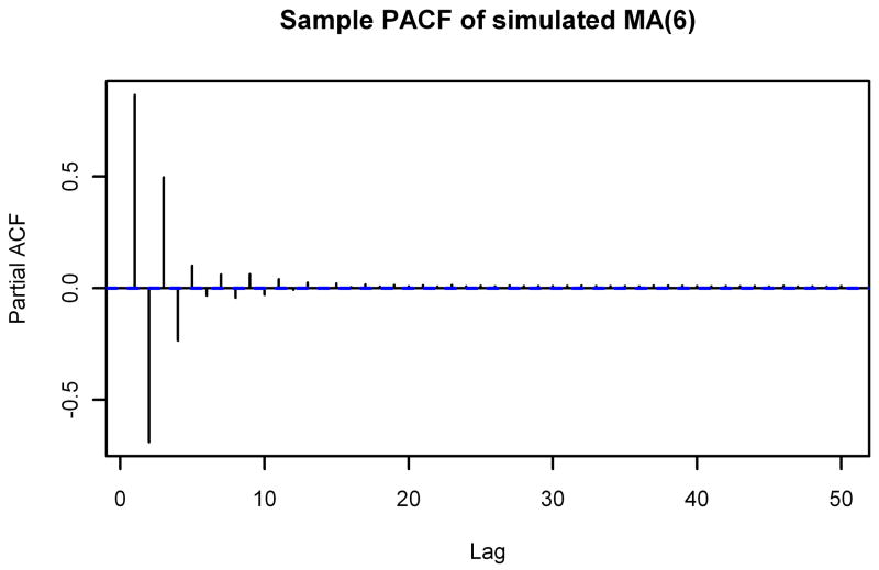
In addition, we see that the sample ACF and sample PACF of the simulated spectrum match those of the actual noise spectrum quite well. The sample ACF of a spectrum simulated from an MA(6) model also closely matches the sample ACF of the noise spectrum, but the sample PACFs are noticeably different. Figure 5 shows the sample PACF of the simulated spectrum from Figure 4 along with the sample PACF of a spectrum simulated from an MA(6) model. It is clear that the sample PACF of the MA(6) model does not decay nearly as quickly as the sample PACF of the noise spectrum, but the sample PACF of the spectrum simulated from the ARMA(1,5) model matches very well.

Figure 5.

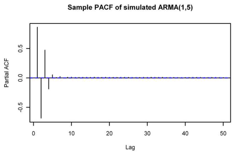
Sample PACFs of Simulated Spectra. The sample partial autocorrelation functions through lag 50 of spectra simulated using the ARMA(1,5) model (top) and an MA(6) model (bottom). Compare to the bottom part of Figure 2.

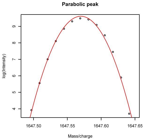
Another result of the ARMA representation of the noise is the explanation of an interesting phenomenon that had been previously observed in MALDI FT-ICR spectra. Barkauskas, et al. [3] used a criterion for peak location and quantification that involved taking a shifted logarithm of baseline-corrected data, then finding five consecutive points which, when fitted with a quadratic function, had a negative coefficient for the quadratic term and a correlation satisfying r² ≥ 0.98 (see Figure 6). They observed that typical MALDI FT-ICR spectra have roughly 104,000 such non-overlapping peaks, which clearly indicates that they must be mostly noise and not actual compounds. With spectra simulated as in this article, we get an average of approximately 98,000 such peaks in each spectrum, so it turns out that the proliferation of peaks is probably largely due to the combination of the ARMA(1,5) model and the choice of distribution for the innovations. (Spectra simulated from the same ARMA(1,5) model using normal innovations had only 70,000 such peaks on average, illustrating the dependence on the distribution used for the innovations. Spectra simulated from an MA(6) model with generalized gamma innovations had only 90,000 such peaks on average, which serves as further confirmation that the ARMA(1,5) model is superior.)

Figure 6.

Parabolic Peak. A typical peak in a MALDI FT-ICR spectrum is approximately parabolic.

4 Application: beer spectrum

As an application of the techniques developed in the previous sections, we use them to detect peaks in a MALDI FT-ICR spectrum (shown in Figure 7) generated with beer as the analyte. (Beer was chosen because of its known composition with highly-structured mass patterns of glycans, the compounds of interest in the analysis in Barkauskas, et al. [3]). For a peak-detection criterion, we choose all “large” peaks, which we define as follows: we first take all local maxima in the spectrum which are k times the value of a baseline estimated using an improved version of a method of Xi and Rocke [8] (new version of algorithm submitted for publication), where k is a constant to be determined. We then use a logarithmic transformation on the data and for each maximum look for a set of five consecutive points containing that maximum which, when fitted with a quadratic function, has a negative coefficient for the quadratic term and a correlation satisfying r² ≥ 0.98 as in Barkauskas, et al. [3]. (The taking of logarithms is justified because the data has constant coefficient of variation, so it follows from the δ-method (see, e.g., Bickel and Doksum [9, Theorem 5.3.3]) that taking the logarithm will approximately variance-stabilize the data, which will allow for the direct application of standard linear statistical models for analysis.)

Figure 7.

Spectrum with Analyte. A MALDI FT-ICR spectrum produced using beer as the analyte.

For this article, we choose k to be such that the spectrum being larger than k times the estimated baseline is roughly equivalent to being n standard deviations above the mean for n ∈ {4, 4.25, 4.5, 4.75, 5} in an independent, identically-distributed normal situation (i.e., we want the Φ(n) quantile of the assumed distribution.) To estimate k, we ran 100 simulations of 10⁷ observations of ARMA(1,5) data generated with coefficients from Table 1 and innovations given by a generalized gamma distribution with the exponent and shape parameter from Table 1 and scale parameter equal to 1, then scaled the observations so each sample mean was 1. For each simulation we calculated the observed Φ(n) quantile of the data (i.e., k) for each of the five choices for n. The estimated values of k and their standard deviations are displayed in Table 2. The choice of k then boils down to a sensitivity/specificity debate. If the primary goal is discovery, then a lower threshold for “large” peaks might be useful; if it is necessary to limit the number of false discoveries, then a higher threshold for “large” peaks would be better.

Table 2.

Estimated Quantiles of the ARMA(1,5) Distribution

	σ-equivalent
Est.	4	4.25	4.5	4.75	5
k̄	3.5059	3.6546	3.7996	3.9377	4.0708
s(k)	0.0087	0.0138	0.0229	0.0364	0.0617

NOTE: “σ-equivalent” refers to the equivalence of the quantiles with the quantiles of the normal distribution that are 4, 4.25, 4.5, 4.75, and 5 standard deviations above the mean. k̄ is the mean and s(k) is the standard deviation of the 100 estimates of k.

For comparison, we also looked for “large” peaks using a simple threshold model with the threshold chosen using Tukey’s biweight with K = 9 to calculate robust measures of center c and scale s for the spectrum, then proceeding as above by starting with any local maximum which was at least c + 9s and looking for parabolic peaks.

We classified the peaks found by any of these methods as being either glycans, fragments of glycans, or unknown peaks. We then further subdivided the unknown peaks into those that had at least one isotope peak that was also detected by at least one method and those for which the main peak was the only peak ever detected. The presence of at least one detected isotope peak virtually guarantees that the peak is an actual compound, while a peak with no isotope peaks detected could be either (i) a real compound whose abundance is so low that its isotope peaks are lost in the noise, or (ii) some type of noise—for example, an electronic spike like those from the noise spectrum in Figure 1. The results of each of these procedures applied to the beer spectrum are summarized in Table 3, along with the same procedures applied to the noise spectrum from Figure 1.

Table 3.

Number of Peaks Found in Beer Spectrum and Noise Spectrum

	σ-equivalent
	4		4.25		4.5		4.75		5		Threshold
Type of peak	PP	Iso	PP	Iso	PP	Iso	PP	Iso	PP	Iso	PP	Iso
Sugar	27	55	27	55	27	54	27	54	27	54	27	55
Fragment	165	203	160	195	155	190	151	182	150	173	169	209
Unknown, with isotope	12	11	11	10	11	10	11	8	11	8	13	18
Unknown, w/o isotope	81	—	53	—	35	—	27	—	21	—	86	—
Noise spectrum peaks	30	—	12	—	5	—	3	—	2	—	34	—

NOTE: “PP” is the number of primary peaks detected; “Iso” is the number of isotopes of primary peaks detected (not counting the primary peaks).

By examining the masses of the peaks detected by each method, it is clear that the threshold method is preferentially selecting peaks at higher masses (lower frequencies). This is due to the fact that the mean levels of MALDI FT-ICR spectra are basically increasing functions of mass, so naturally peaks at the higher masses will have a greater chance of being above the chosen threshold value. What might be surprising at first glance, however, is that the σ-equivalent methods are preferentially selecting peaks at lower masses (higher frequencies). If the model is correct, the detected peaks should consist of signal, which should be detected no matter which method is used; and noise, which should be approximately uniformly distributed throughout the spectrum. This apparent contradiction can be resolved by observing that because of the form of the transformation used to calculate mass from frequency, the vast majority of the data points are at low masses. When the masses are translated back to frequencies, we see that the peaks detected in the noise spectrum by the σ-equivalent methods are at frequencies that are roughly uniformly distributed throughout the spectrum (Figure 8), as expected. In addition, the σ-equivalent methods are clearly doing a better job of not detecting peaks in the noise spectrum. Thus, the σ-equivalent methods appear to be the correct ones to use for peak detection.

Figure 8.

Peak Detection Method Comparison. Peaks detected in noise spectrum by 4σ-equivalent method and threshold method, plotted by mass (top) and by frequency (bottom). Note that low masses correspond to high frequencies and vice versa.

5 Future directions

One obvious future direction is to implement a maximum-likelihood estimation algorithm following the methods of Li and McLeod [7] to find simultaneous estimates of the ARMA coefficients in Equation (7) and the parameters α and β from Equation (6) as well as standard errors for the estimates of α and β. Another is to explore models for the innovations other than the generalized gamma distribution.

Another possible direction is based on the observation that all of the spectra analyzed in this article were generated on the same machine; it would be interesting to see how much of this is machine-dependent by analyzing spectra from other MALDI FT-ICR MS machines. The ideal situation would be if one could calculate α, β, and (possibly even) {μ_t} once for each machine and then use these values for analysis going forward. In any case, the framework provided in this article should allow other researchers to determine appropriate parameters for their own MALDI FT-ICR mass spectrometry setups.

References

- 1.Herbert CG, Johnstone RAW. Mass Spectrometry Basics. CRC Press; Boca Raton, FL: 2003. [Google Scholar]
- 2.Park Y, Lebrilla CB. Application of Fourier transform ion cyclotron resonance mass spectrometry to oligosaccharides. Mass Spec Rev. 2005;24(2):232–264. doi: 10.1002/mas.20010. [DOI] [PubMed] [Google Scholar]
- 3.Barkauskas DA, An HJ, Kronewitter SR, de Leoz ML, Chew HK, de Vere White RW, Leiserowitz GS, Miyamoto S, Lebrilla CB, Rocke DM. Detecting glycan cancer biomarkers in serum samples using MALDI FT-ICR mass spectrometry data. Bioinformatics. 2009;25(2):251–257. doi: 10.1093/bioinformatics/btn610. [DOI] [PMC free article] [PubMed] [Google Scholar]
- 4.Zhang LK, Rempel D, Pramanik BN, Gross ML. Accurate mass measurements by Fourier transform mass spectrometry. Mass Spec Rev. 2005;24(2):286–309. [Google Scholar]
- 5.Shumway RH, Stoffer DS. Time Series Analysis and Its Applications with R Examples. 2. Springer; New York, NY: 2006. [Google Scholar]
- 6.Hurvich CM, Tsai CL. Regression and time series model selection in small samples. Biometrika. 1989;76(2):297–307. [Google Scholar]
- 7.Li WK, McLeod AI. ARMA modelling with non-Gaussian innovations. J Time Series Analysis. 1988;9(2):155–168. [Google Scholar]
- 8.Xi Y, Rocke DM. Baseline correction for NMR spectroscopic metabolomics data analysis. BMC Bioinformatics. 2008 Jul;9 doi: 10.1186/1471-2105-9-324. [DOI] [PMC free article] [PubMed] [Google Scholar]
- 9.Bickel PJ, Doksum KA. Mathematical Statistics. 2. Vol. 1. Prentice Hall; Upper Saddle River, NJ: 2001. [Google Scholar]