Estimation efficiency and statistical power in arterial spin labeling fMRI

Abstract

Arterial spin labeling (ASL) data are typically differenced, sometimes after interpolation, as part of preprocessing before statistical analysis in fMRI. While this process can reduce the number of time points by half, it simplifies the subsequent signal and noise models (i.e., smoothed box-car predictors and white noise). In this paper, we argue that ASL data are best viewed in the same data analytic framework as BOLD fMRI data, in that all scans are modeled and colored noise is accommodated. The data are not differenced, but the control/label effect is implicitly built into the model. While the models using differenced data may seem easier to implement, we show that differencing models fit with ordinary least squares either produce biased estimates of the standard errors or suffer from a loss in efficiency. The main disadvantage to our approach is that non-white noise must be modeled in order to yield accurate standard errors, however, this is a standard problem that has been solved for BOLD data, and the very same software can be used to account for such autocorrelated noise.

Introduction

Arterial spin labeling (ASL) techniques have been in development for over a decade since their inception (Williams et al., 1992), but it was not until more recently that arterial spin labeling was shown to be a very powerful technique for functional imaging of low-frequency paradigms (Aguirre et al., 2002; Wang et al., 2003). Further improvements in the technique have made it a practical tool for functional MRI of high-frequency (i.e., event related) paradigms by overcoming issues of temporal resolution, SNR, and the ability to collect multiple slices in a single TR (Wong et al., 2000; Hernandez-Garcia, 2004; Silva et al., 1995). ASL is inherently a low signal to noise ratio (SNR) technique so it is important to maximize the accuracy and sensitivity of the analysis.

ASL techniques are very appealing for functional imaging primarily because they offer a physiologically meaningful and quantitative alternative to BOLD effect imaging, currently the dominant technique used for functional brain mapping. In summary, ASL consists of acquiring image pairs made up of a “labeled” image, in which the inflowing blood has been magnetically labeled, and a control image without labeled blood. Perfusion can be calculated from the difference of those two images, which is made up only of the labeled blood present in the imaged slice. The subtraction of image pairs results in an added benefit, namely that the subtracted data contain noise that is whiter than BOLD noise (Aguirre et al., 2002; Wang et al., 2003), depending on the specific subtraction scheme used for obtaining the labeled images from the raw ASL images (Liu and Wong, 2005).

In this article, we consider data collected using the Turbo-CASL sequence. Turbo-CASL is a spin labeling technique that takes advantage of the delay period between labeling spins at the neck and the time they reach the imaging plane to collect the control image, resulting in a more efficient use of the time. This technique is obviously quite sensitive to transit times, so one must collect a transit time measurement and adjust the timing parameters of the sequence accordingly. The benefits of the technique are an increase in the temporal resolution while preserving some of the higher SNR characteristics of continuous ASL and the ability to obtain exaggerated activation responses by proper choice of labeling parameters. The drawbacks are that it requires knowledge of transit times and that excessive variability of those transit times over the imaged tissue can result in SNR loss in some regions (Hernandez-Garcia et al., 2004, 2005; Lee et al., 2004).

Despite the simplicity of the subtraction analysis method, it cannot strictly be optimal for estimation and detection of brain activity using the general linear model. For a given linear model of the full (length-N) dataset, the Gauss–Markov Theorem (Graybill, 1976) dictates that optimally precise estimates are obtained from ordinary least squares (OLS) estimates for independent data, or from whitened OLS (i.e., generalized least squares, GLS) for dependent data. Therefore, since the full-length ASL time series suffers from temporal autocorrelation, OLS is not appropriate. Also since differencing the data is not equivalent to whitening, differencing is suboptimal to GLS.

The goal of this work is to characterize the statistical properties of different ASL modeling methods. Starting from a general linear model that includes the alternating control-label effect, we examine several differencing schemes including a no-differencing approach. To measure goodness of the differencing schemes, we calculate the bias of the variance estimators, the estimation efficiency and the estimator power for different study designs and error covariance structures. We also analyze real data to produce a comparison of Z scores between the models and explain the results in the context of signal processing.

Theory

We first describe the signal model, then the differencing methods and their frequency responses, then the noise model used and, finally, the estimation methods.

Signal model

We pose the signal model for ASL data in terms of a General Linear Model (GLM). While Liu et al. (2002) posed a separate GLM for control and label data, we consider a single model for the collected data,

$$Y=X\beta +\mathrm{\epsilon }$$ (1)

where Y is a vector of length N that contains the original experimental data ordered as acquired, including labeled and non-labeled images; X is a N × p design matrix; β is a vector of p parameters; and ε is the error vector of length N where Cov(ε) = σ²V. When autocorrelation is modeled, the X matrix will typically be appended with columns to account for low-frequency, non-stationary variation. For clarity, we omit these predictors in the following but revisit them in the discussion.

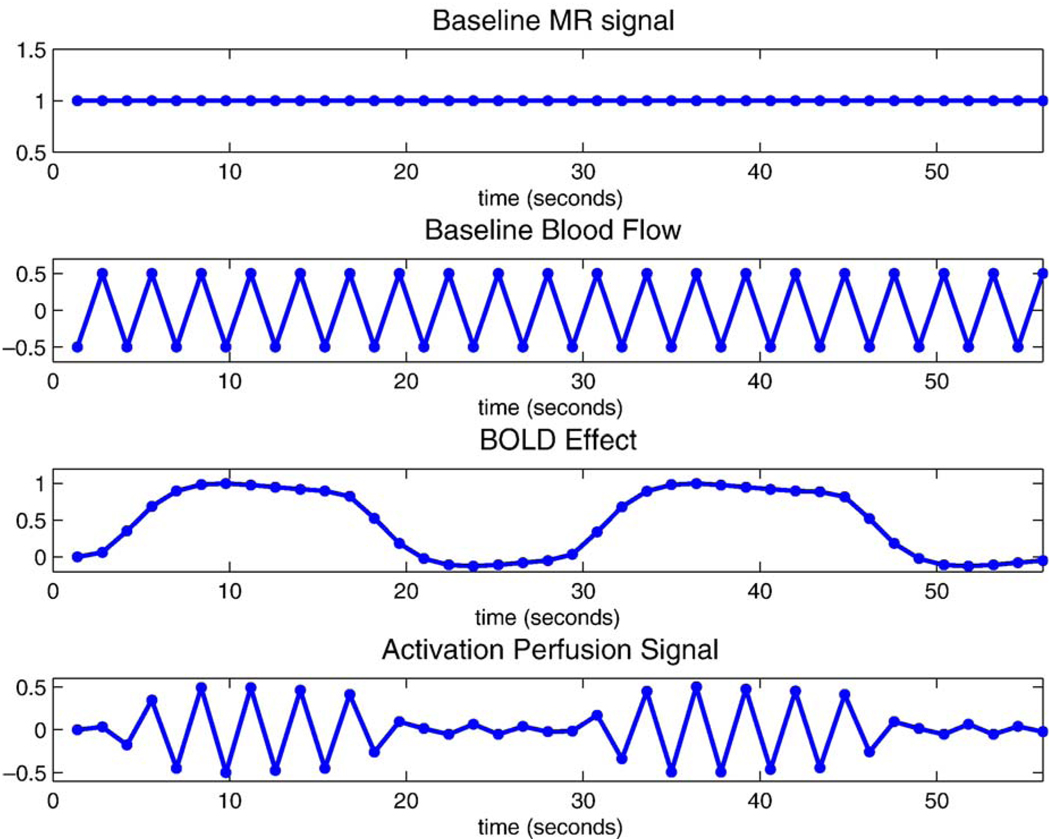
The design matrix for our experimental conditions was built to reflect the principal contributions to the observed ASL signal. This signal is made up of two fixed baseline components and two dynamically changing components that are due to hemodynamic changes induced by the stimulation paradigm.

The two fixed components are the MR signal from static tissue, which makes up the bulk of the image, and the inflowing blood signal in the baseline state. The baseline MR signal is just constant in time, while the inflowing blood signal (or baseline blood flow) is sensitive to whether the tag is applied or not (top panel, Fig. 1). Hence, the baseline blood flow regressor is simply a function of alternating positive and negative values, +a and −a, depending on whether the tag is applied or not. While alternating 1 ’s and −1 ’s (a = 1) seems natural for this predictor, instead a = 1/2 should be used so that the corresponding parameter expresses a unit effect in the data. Note that the presence of the arterial tag corresponds to −a, since the tag is made of inverted spins, and hence reduces the total signal magnitude (second panel Fig. 1). It also should be noted that estimation of this regressor does not yield an absolute quantitative measure of baseline perfusion.

Figure 1.

Predictors used in GLM for collected data (first 40 time points). The top two figures show baseline MR signal and baseline blood flow regressors and the bottom two figures show the BOLD effect and activation perfusion signal regressors. Note that the baseline blood flow predictor ranges from −0.5 to 0.5; this is done so that the corresponding parameter in the model represents a unit effect in the data.

The two activation-related regressors are the perfusion changes and the BOLD effect changes in signal, generated by convolution of the stimulation function with a gamma-variate BOLD response function (third panel, Fig. 1). The changes in perfusion due to activation are known to have similar temporal properties to those in the BOLD response, but they are sensitive to the presence of the arterial inversion tag. Thus, in order to capture the perfusion changes due to activation, we created the activation perfusion regressor by modulating the BOLD regressor with the baseline blood flow regressors to reflect the presence or absence of the inversion tag (fourth panel, Fig. 1).

The observed MR signal is thus made up of the weighted sum of these four components, or regressors, which are depicted in Fig. 1.

Differencing methods

Differencing the data can be built into the model by premultiplying both sides of the GLM equation by a generic differencing matrix, D:

$$\mathit{\text{DY}}=\mathit{\text{DX}}\beta +D\mathrm{\epsilon }.$$ (2)

Any differencing scheme can be encompassed in this model by specification of an appropriate D. We denote D₁ = I, where I is a N × N identity matrix, for the case of no differencing at all. The standard pairwise differencing can be implemented with a N/2 × N differencing matrix

$$D_2=\left(\begin{array}{ccccccc}1& -1& & & & & 0\\ & & 1& -1& & & \\ & & & & \ddots & & \\ 0& & & & & 1& -1\end{array}\right)$$

The other differencing approaches we study include running subtraction, with (N − 1) × N differencing matrix

$$D_3=\left(\begin{array}{cccccc}1& -1& & & & 0\\ & -1& 1& & & \\ & & 1& -1& & \\ & & & \ddots & \ddots & \\ 0& & & & 1& -1\end{array}\right),$$

surround subtraction with (N − 2) × N differencing matrix,

$$D_4=\left(\begin{array}{ccccccc}1& -2& 1& & & & \\ & -1& 2& -1& & & \\ & & 1& -2& 1& & \\ & & & \ddots & \ddots & \ddots & \\ & & & & -1& 2& -1\end{array}\right)$$

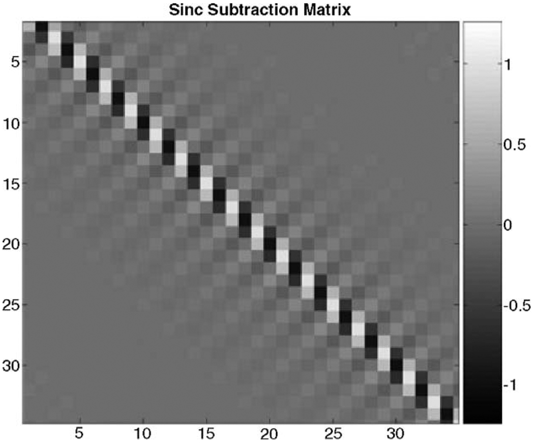
and sinc subtraction (D₅). The N × N differencing matrix for sinc subtraction is best illustrated as an image of the differencing matrix, as in Fig. 2.

Figure 2.

Example of a differencing matrix that implements a sinc subtraction (differencing matrix D₅).

Noise model

It is well known that the elements of the error, ε are not independent, with Cov(ε) = σ²V being non-diagonal. For example, Zarahn et al. (1997) found that the power spectra of fMRI noise data follow a “1/f ” frequency–domain structure, which is associated with a lower order autoregressive (AR) model. In the evaluations below, we will use an AR(1) plus white noise (WN) model; we found this autocorrelation structure to follow that of our data through empirical observations. Such a model has an autocorrelation structure, V, where the correlation for a lag of 𝓁 is defined by

$$V_{k,k-𝓁}={\rho }^{\left|𝓁\right|}\left(\frac{{\sigma }_{\text{AR}}^2}{{\sigma }_{\text{AR}}^2+{\sigma }_{\text{WN}}^2}\right)$$

and the variance of each measurement is given by ${\sigma }^2={\sigma }_{\text{AR}}^2+{\sigma }_{\text{WN}}^2$ where ${\sigma }_{\text{AR}}^2$ is the variance contributed from the AR(1) process, ${\sigma }_{\text{WN}}^2$ is the white noise variance and ρ is the AR(1) correlation parameter.

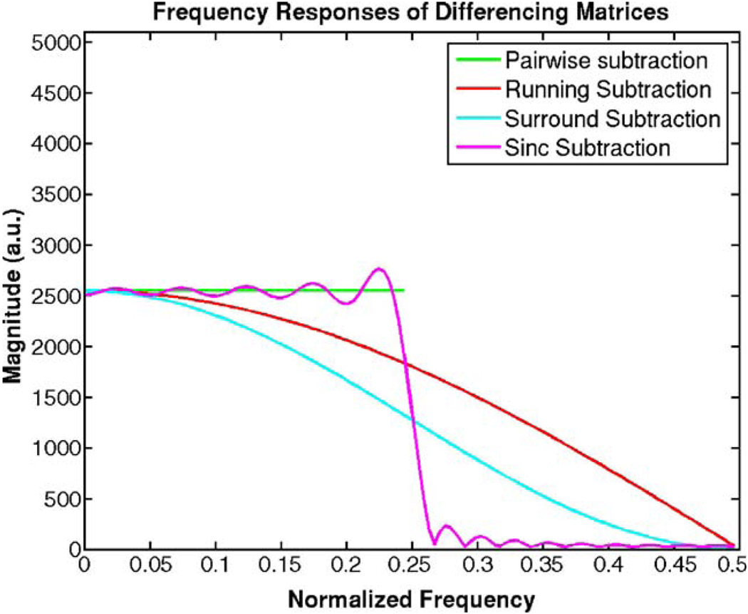
The effect of differencing matrices on the noise can be thought of as a two-step process: either aliasing (in the cases of pairwise and sinc subtractions) or demodulation (in the cases of running and surround subtractions), followed by a low pass filter. The effect of demodulating the system by the Nyquist frequency on the frequency spectrum is to shift the spectral content of the signal by π rad/s. The effect of subsampling (aliasing) by a factor of two on the frequency spectrum is to “reflect” the spectral content such that the top half of the spectrum is reversed and added on to the lower half. The resulting spectra can be derived analytically for a given input y[n] whose discrete Fourier transform is white and given by Y(e^jw). The derivations are showed in appendix B, and the results of the derivations are summarized in Table 1. Plots of the outputs of the different systems are shown in Fig. 3 as a function of the normalized continuous time frequency.

Table 1.

Frequency responses of the differencing schemes

Type of differencing		Fourier domain expression
D1	No subtraction	$Y_1(e^{j\omega })=Y\left(\begin{array}{c}j\omega \\ e\end{array}\right)$
D2	Pairwise subtraction	Y2(ejω) = 0.5·[ Y(ejω/2)(1-ejω/2) + Y(ej(ω+ 2π)/2)(1-ej(ω+2π)/2)]
D3	Running subtraction	Y3(ejω) = Y(ej(ω+π))(1-ej(ω+π))
D4	Surround subtraction	Y4(ejω) = Y(ej (ω+π))(− 1 + 2ej(ω+π) − e 2j(ω+π))
D5	Sinc subtraction	Y5(ejω) = Y2(ej 2ω)S(ejω )*

^*Y_2z = is the Fourier transform of y_2z[n], which is in turn the same as y₂[n] (the time domain output of the pairwise subtraction case) but zero filled between samples. In an ideal case (an Infinite Impulse Response filter), S would be a perfect rect function but, depending on the implementation, it is the Fourier transform of a truncated sinc function instead, and is dependent on the choice of truncated sinc.

Figure 3.

Expected output frequency spectra as predicted by the equations in Table 1. Note that these are the responses after the demodulation step in the equation. They correspond to each of the differencing matrices, which combine the filtering and demodulating effects into a single step.

Liu and Wong (2005) took a similar signal-processing approach in order to examine the effects of differencing on the BOLD and perfusion responses observed in ASL functional time series data, including BOLD effects (an ASL sequence in which the acquisition is carried out with a gradient echo with a long echo time would also be BOLD weighted). By modeling the acquisition scheme as a linear system, they also noted that the control-label modulation shifts the activation to higher frequencies in the BOLD weighted data and the choice of differencing method is contingent on the spectral content of the time series (determined by the experimental design).

Pairwise subtraction and sinc subtraction do not have a straightforward linear response since they both involve down-sampling the data prior to subtraction, although sinc-subtraction subsequently upsamples the data in the two separate channels. In both of those cases, the downsampling process causes the top half of the frequency spectrum to demodulate (shift in frequency) the signal into the bottom half before the filtering process (see Fig. 3). In terms of their frequency responses, they are very similar except for the imperfections of the sinc kernel used in the implementation. In terms of detection and statistics, sinc subtraction preserves greater degrees of freedom than pairwise subtraction, which reduces the number of time points by half. It is interesting to note that pairwise subtraction yields the same result as downsampling the running subtraction.

Estimation

Based on both the differenced and undifferenced data, OLS or GLS can be used to estimate and make inference on β. While OLS estimates of β are unbiased even when data are temporally autocorrelated, the estimates do not have minimum variance, meaning they are not fully efficient; further, the estimated standard errors are biased, which can result in test statistics that are either too large or too small. The optimal approach is GLS, corresponding to OLS on the whitened data and model, and is implemented in most fMRI packages (e.g., FSL and SPM). GLS requires that the structure of the noise in the data be known or, at least, estimated with high precision. The noise covariance, σ²V, is estimated by a variety of means (Worsley et al., 2002; Friston et al., 2002; Woolrich et al., 2001); most methods use a regularized fit of a low-dimensional autocorrelation model to the OLS residuals.

Given that the covariance of the error,ε, is σ²V, the covariance of the error of the differenced data, Dε, is given by ${\sigma }^2{\mathit{\text{DVD}}}^T={\sigma }_D^2{V}_D$ where ${\sigma }_D^2$ is the variance of the differenced error and V_D is the corresponding autocorrelation¹. Let W be a whitening matrix such that W(V_D)W^T = I the whitened version of the general linear model is then

$$\mathit{\text{WDY}}=\mathit{\text{WDX}}\beta +\mathit{\text{WD}}\mathrm{\epsilon }$$ (3)

and the GLS estimate of β is given by

$$\widehat{\beta }={(\mathit{\text{WDX}})}^{-}\mathit{\text{WDY}},$$ (4)

where the symbol ⁻ denotes a pseudo-inverse operator (Graybill, 1976, p. 28). The variance of the estimate is given by

$$\text{Var}\left(\widehat{\beta }\right)={(\mathit{\text{WDX}})}^{-}[{\mathit{\text{WV}}}_D{W}^T]{({(\mathit{\text{WDX}})}^{-})}^T{\sigma }_D^2.$$ (5)

If the whitening is accurate, the middle bracketed term will be identity; however, if OLS is used, then W = I and this term will not vanish.

Two problems may arise with the estimation procedure. First, if D ≠ I the intercept predictor in X will become an all-zero predictor in DX; for example, in the case of simple subtraction, the N-vector intercept [1, 1,…, 1] becomes a N/2 vector of zeros and should be omitted. More generally, effects nullified by D can be removed by an appropriate transformation, resulting in a reduced number of columns. Second, D’s may induce linear dependencies into DY, resulting in a singular covariance matrix V_D = DVD^T; for example, a N-by-N sinc subtraction matrix has rank N − 1. This problem can be resolved by removing rows of D until V_D is positive definite.

The residual variance is estimated with the residual mean square of the whitened differenced data,

$${\hat{\sigma }}_D^2=\frac{1}{N-p}{(\mathit{\text{WDY}}-\mathit{\text{WDX}}\widehat{\beta })}^T(\mathit{\text{WDY}}-\mathit{\text{WDX}}\widehat{\beta }).$$ (6)

Then the estimated variance, $\widehat{\text{Var}}(\widehat{\beta })$, is found by substituting ${\widehat{\sigma }}_D^2$ into Eq. (5). Note that under OLS, it is assumed that V_D = W = I, while with GLS the assumption is W(V_D)W^T = I.

The T test for the null hypothesis H₀: cβ = 0 $T=c\widehat{\beta }/\sqrt{\widehat{\text{Var}}(c\widehat{\beta })},$ where c is a contrast used to express the effect of interest.

Methods: model evaluation

Model details

For a given times series with length N = 258 (TR = 1.4 s) where the temporal autocorrelation followed an AR(1) + WN structure, a signal model for a TurboCASL perfusion experiment was created for three different experimental designs: a fixed ISI event-related design (ISI = 18, SOA= 20, stimulus duration = 2 s), a randomized event-related design (uniform distribution, 5 < ISI < 12 s), and a blocked design (30 scans ON, 30 scans OFF). The randomized event-related design was repeated 100 times to verify consistency across different realized designs. Appropriate general linear models were created consisting of baseline image intensity, baseline blood flow, BOLD response and increases in perfusion due to activation. The perfusion responses were modeled as a difference of two gamma variate functions.² Fig. 1 graphically illustrates the first 60 s of the first subject’s design matrix’s regressors for a block design.

Efficiency and bias

The efficiency of the estimated contrast, cβ̂, from the different models is given by the reciprocal of the true variance, 1/Var(cβ̂). If one method is less efficient than another method, it is not as sensitive for the detection of effect cβ.

The biases of ${\widehat{\sigma }}_D^2\text{and}\widehat{\text{Var}}(c\widehat{\beta })$ for the differencing models under the assumptions of OLS were also calculated. The derivations of these quantities are given in Appendix A. If these estimates are biased, it indicates that the differenced data are correlated, hence violating the OLS assumption of independent measurements and resulting in test statistics that can be too large or too small.

We computed the efficiency of the contrast estimated and bias of the estimated variance over a range of AR(1) + WN models. Specifically, we studied a range of AR parameter values (ρ) between 0 and 0.9. Also, since all values of ${\sigma }_{\text{AR}}^2\text{and}{\sigma }_{\text{WN}}^2$ that share the same ${\sigma }_{\text{AR}}^2/{\sigma }_{\text{WN}}^2$ yield the same relative efficiency and bias values, we varied the variance of the AR(1) + WN by varying the ratio, ${\sigma }_{\text{AR}}^2/{\sigma }_{\text{WN}}^2$, between 0 and 25.

Statistical power

Power is the probability of detecting a given effect of magnitude cβ with a given significance level. Power estimates are not meaningful when $\widehat{\text{Var}}(c\widehat{\beta })$ is biased; for example, negative bias leads to an overestimation of power since the test statistics are artificially large. Hence, we followed what is standard practice in the statistics literature, and only considered statistical power for methods where $\widehat{\text{Var}}(c\widehat{\beta })$ was found to be unbiased; this included the no differencing model estimated with GLS and the pairwise subtraction model estimated with OLS. We calculated power over a range of the signal to noise ratio (SNR = change in perfusion/σ). SNR was varied by varying the change in perfusion between 0.1 and 2 and fixing the variance at 1.45. The details of the power calculation are described in Appendix A.

Methods: imaging data

Data collection

All imaging was carried out using a 3.0 T Signa LX scanner (General Electric, Milwaukee, WI, USA) fitted with an additional, home-built, spin labeling system. Double-coil turboCASL time series data collected from six subjects during a finger tapping event-related experiment (4 slices, FOV = 24 cm, ISI = 18 s, 360-s duration, TR = 1.4 to 1.6 s depending on resting transit time, GE spiral, TE = 12 ms). Prior to acquisition of time series data, the sequence was optimized for each individual subject by collecting a set of Turbo-CASL images with varying TR (800, 1200, 1400, 1600, 1800, 2000, 2200 and 4000 ms). Labeling time was always 200 ms less than TR. The parameters that produced the highest SNR were chosen as the optimum TurboCASL regime as in Hernandez-Garcia et al. (2004). K-space data were filtered to remove spurious RF noise that may be introduced by the labeling coil and reconstructed using field map homogeneity correction.

Data analysis

While there are 10 possible methods (OLS and GLS for 5 differencing methods), we only considered two to be practical with real data: GLS with no differencing (D₁) and OLS with simple subtraction (D₂). OLS is inappropriate with any method other than simple subtraction because the errors are not independent (non-white noise). While the error autocorrelation of other differencing methods (DVD^T) could feasibly be estimated, existing fMRI software is designed to estimate V in undifferenced time series, and hence, we only used GLS with the original data.

For each subject, at each voxel, a GLS model with no differencing was fit with the FEAT software tool, which is part of fMRIB’s software library FSL.³ FSL estimates an autocorrelation function (ACF) at each voxel and, after tapering and non-stationary spatial smoothing, constructs V for data and model whitening. When whitening, we also included a high pass temporal filter to remove low-frequency artifacts. The high pass filter in FSL uses a local fit of a straight line, where Gaussian weighting within the line is used to give a smooth response. The simple subtraction data was also fit with FEAT, but without whitening. T statistics were converted to Z statistics with a probability integral transform. The Z statistics from each analysis were then compared. Both methods should yield valid inferences, that is, null-hypothesis voxels should have comparable Z statistics; but when a signal is present, larger Z values are evidence of greater sensitivity. A sign test on the median difference in z scores is computed over subjects to detect consistent effects.

To assess the assumption of independence in the differenced data we separately ran the simple difference data through SPM and SPMd (Luo and Nichols, 2003). From SPMd, we obtained power spectrum of the residuals, averaged over brain voxels, and diagnostic-log10 P value images for testing AR(1)-type positive autocorrelation (“Corr”) and arbitrary correlation (“Dep”). We summarize the diagnostic images by whether one or more voxels surpassed a 0.05 Bonferroni threshold.

Frequency response

Active voxels were identified by correlation analysis with a reference function generated using the stimulus presentation function convolved with a gamma variate function. Voxels whose t score was above 3 (r > 0.2) and had at least one supra-threshold neighbor were classified as active. Time courses (length = 258 points) were extracted from those active voxels (N = 87) and from 87 non-active voxels in the frontal lobe. Frequency spectra were computed from the undifferenced and differenced data and compared to the frequency spectra obtained from applying the predicted frequency response function to the raw data.

Results

Power and efficiency calculations

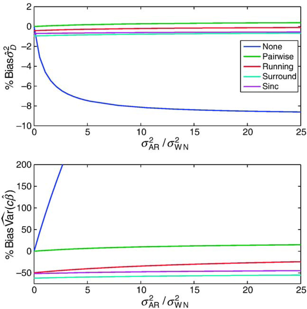
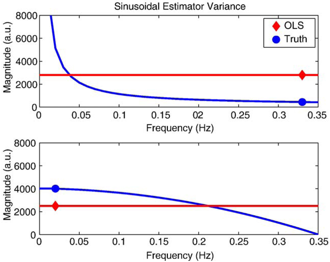
Three experimental design types were considered, as described in the Methods: model evaluation section: blocked, randomized event-related and fixed event related. For the reasons described above, OLS was used to estimate all differencing models and GLS was only used in the no differencing case. Fig. 4 illustrates the percent biases in both ${\widehat{\sigma }}_D^2\text{and}\widehat{\text{Var}}(c\widehat{\beta })$ when OLS is used to estimate the differencing models. When bias is present, it is an indication that there is autocorrelation or variability in the data that the model is ignoring. The top panel shows the bias in ${\widehat{\sigma }}_D^2$, where the no subtraction model results in strong negative bias while the running, surround and sinc subtraction models have a slightly negative bias and the pairwise differencing model has almost no bias. The direction of the bias in ${\widehat{\sigma }}_D^2$ is in the opposite direction of the autocorrelation that is ignored; hence, negative bias indicates positive autocorrelation (Berry and Feldman, 1985, p. 78). The bottom panel illustrates that $\widehat{\text{Var}}(c\widehat{\beta })$ has negative bias in all cases except for the simple subtraction model, which has appreciable positive bias. To understand these results, Fig. 5 shows an illustration of two cases, that of no differencing and running subtraction. Shown are the true noise spectra in blue, and the flat noise spectra implied by OLS in red, and the estimator variance for a sinusoidal experimental predictor. The top panel shows how OLS with no differencing overestimates power at high frequencies, where the modulated perfusion signal is, leading to positive bias. The bottom panel shows how an OLS running subtraction model overestimates variance at low frequencies, where the differenced signal is, producing negative bias.

Figure 4.

Bias of ${\widehat{\sigma }}_D^2\text{and}\widehat{\text{Var}}(c\widehat{\beta })$, expressed as percent of true variance, for subtraction methods using OLS for different AR(1) + WN variance models. The study design used was the block design and the AR parameter, ρ, was fixed at 0.9.

Figure 5.

Illustration explaining the directions of the bias of the estimated variance for the cases of no differencing and running subtraction. The top panel shows how OLS with no differencing overestimates power at high frequencies, where the modulated perfusion signal is, leading to positive bias. The bottom panel shows how an OLS running subtraction model overestimates variance at low frequencies, where the differenced signal is, producing negative bias.

To make concrete the magnitude of bias on a P value, consider an example where there is −50% bias in $\widehat{\text{Var}}(c\widehat{\beta })$. If the biased variance is used in the test statistic, a biased P value of 0.01 will be found when the true P value is actually 0.05; similarly a 0.0001 biased P value would be found when 0.004 is actually correct. So the biased variance inflates significance and can lead to an incorrect conclusion of significant activation.

The study design used in Fig. 4 was block design, but results were similar for the event-related designs also. Different values of ρ were also considered and as ρ decreased, the bias in the undifferenced model approached 0, but the percent bias in $\widehat{\text{Var}}(c\widehat{\beta })$ was similar to that shown in Fig. 4 for the other differencing methods (results not shown).

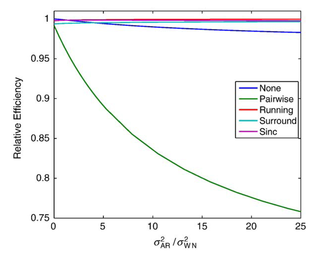
The linear models considered were able to estimate the amplitude of the responses with varying statistical efficiency. Fig. 6 shows the relative efficiency of the model estimation under the block design study, where the differencing models estimated with OLS are compared to no differencing with GLS. The pairwise differencing method shows the greatest loss in efficiency, up to 24% or more, while the other differencing methods are more efficient. The results were similar for the event-related designs, with a slightly larger loss in efficiency for the pairwise subtraction method but the relative efficiency for the other methods remained near 1 (results not shown).

Figure 6.

Estimation efficiency (relative to no differencing, GLS analysis) for subtraction methods using OLS for different AR + WN variance models for a block design study.

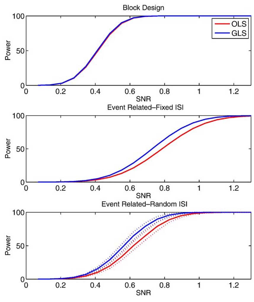
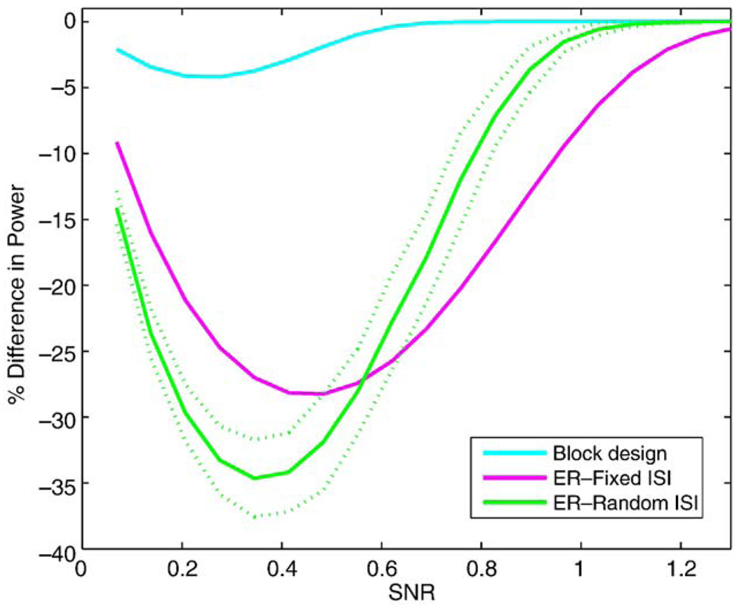
For the power study, we only consider models where $\widehat{\text{Var}}(c\widehat{\beta })$ has little or no bias: simple subtraction using OLS and no differencing with GLS. Fig. 7 shows the power for no differencing with GLS and that of pairwise differencing with OLS for the 3 study designs over SNR values ranging between 0.1 and 1.4. The AR(1) + WN model used had a correlation parameter ρ = 0.90, AR variance, ${\sigma }_{\text{AR}}^2=0.11$ and white noise variance, ${\sigma }_{\text{WN}}^2=2$. The dotted lines on the random event-related figure indicate ±2 standard deviations of the average power over the 100 realizations. The power is similar between the two methods for the block design, which is expected (see Appendix C), but GLS is seen to have larger power for the event-related study designs. Another view of this result is shown in Fig. 8, which shows the ratio of OLS power to GLS power. The random event-related design can have up to 35% (SD 1.5%) lower power when OLS is used compared to GLS. Note that the U-shape to the curves in Fig. 8 is to be expected: when SNR is very small, power is 0 for any method, and hence, there is no percent difference; likewise, when SNR is very large, power is 1 for any method and there is again no difference.

Figure 7.

Power of the no differencing model estimated with GLS and pairwise subtraction estimated with OLS for 3 study designs. Random ISI event-related design indicates average power over 100 iterations (solid) and ±2 standard deviations (dashed).

Figure 8.

Relative Power 100 × (OLS − GLS)/GLS for the different study designs. Random ISI event-related design indicates average relative power over 100 iterations (solid) and ±2 standard deviations (dashed).

Experimental data

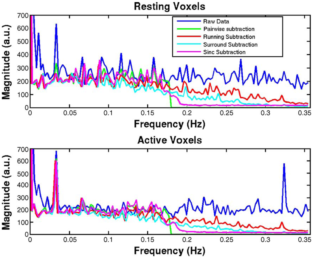
Undifferenced time courses from the experimental ASL time series were extracted from 87 active and 87 resting voxels (identified through simple correlation analysis). The effects of the differencing schemes on the frequency spectra of data can be seen in Fig. 9. The frequency spectra of time courses extracted from resting and active voxels are shown in the top and bottom panels, respectively. The blue line shows the spectral content of the raw (undifferenced) data, the other lines show the effects of simple, running, surround, and sinc subtraction schemes. The appearance of the raw data spectra indicates that our data contain primarily white noise but also a strong AR(1) component $(\rho =0.90,{\sigma }_{\text{AR}}^2=0.11,{\sigma }_{\text{WN}}^2=2)$.

Figure 9.

Frequency spectra of raw and differenced data in Resting (top) and Active (bottom) voxels. (Pairwise subtraction data are zero padded).

The activation-induced perfusion effects, which are typically low frequency by nature, were modulated by the Nyquist frequency because of the alternating acquisition pattern of the control and labeled images. Hence, the activation effects appeared in the higher frequency range in the spectrum. The theory and data agreed that the running and surround subtraction methods demodulated the activation effects back to low frequency and subsequently attenuated the frequency content at the higher frequencies, while the simple and sinc subtraction methods aliased the high-frequency content into the low-frequency range of the spectrum because of the subsampling step. The sinc interpolation kernel produced the smooth roll-off seen at the half-Nyquist frequency. Obviously, the undifferenced data retained all its frequency content. Crucially, only the pairwise subtraction yielded a mostly flat spectrum (for its halved sampling rate), and all other methods had spectra that were more colored than the original data, consistent with our bias calculations above.

Statistical mapping

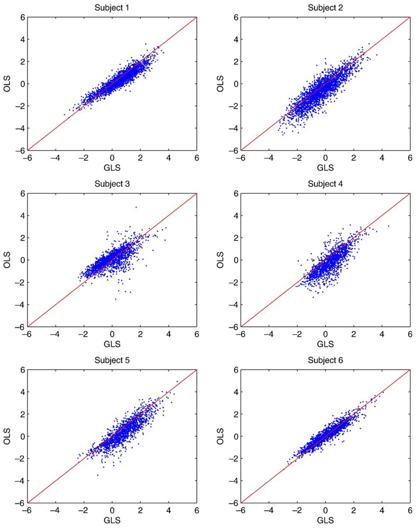
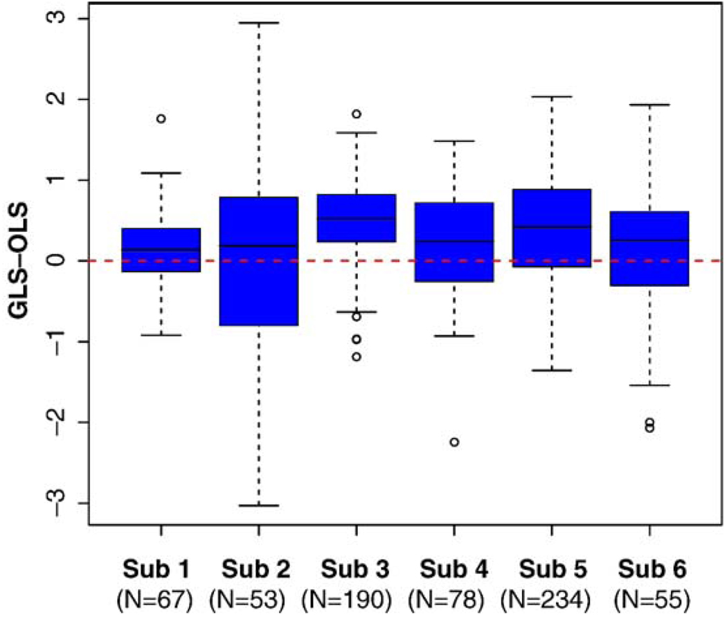
Fig. 10 shows a comparison of Z statistics obtained using GLS with no differencing and OLS with pairwise subtraction in all subjects. These figures show that the Z values for the full model tend to be larger when the statistics are positive and smaller when the statistics are negative, when compared to the subtracted model, which would result in more significant voxels found without differencing and using GLS. Fig. 11 displays the boxplots of the difference in Z values from the two methods when the Z value from either of the methods was larger than 2. Note that boxplots display the distribution of data by showing the median (horizontal black line in box), the first and third quartiles of the data (edges of the blue box), range of points included within 1.5* interquartile range (whiskers) and outliers (points). In all cases, the median is larger than 0 and a sign test for the 7 medians has P = 0.017, indicating that typically the Z value from the undifferenced model using GLS is larger than the differenced model estimated with OLS.

Figure 10.

Comparison of Z values from pairwise differencing for all subjects using OLS and full data using GLS. Note that for most positive values GLS is larger and for most negative values GLS is smaller, indicating greater sensitivity.

Figure 11.

Boxplots of difference in Z values when the Z value from either method was larger than 2. The number of voxels included in each subject’s boxplot are indicated beneath the subject number. Boxplots display the distribution of data by showing the median (horizontal black line in box), the first and third quartiles of the data (edges of the blue box), range of points included within 1.5* interquartile range (whiskers) and outliers (points). Positive values indicate greater sensitivity with full data using GLS.

Based on the strict Bonferroni criterion, 4 out of 6 subjects simple differenced data had evidence of some correlation (1 had significant Corr and Dep, 1 had just significant Corr, and 2 had just significant Dep). This indicates that, despite previous reports, we find not all subject’s produce independent differenced data, due probably to the original noise structure failing to be close to a 1/f structure.

Discussion

Our analysis indicates that the most powerful analysis of ASL data is obtained by using the full data, with no differencing and building the control/label effect into the model implicitly. Using direct calculations and real data, we have found increased sensitivity with this approach relative to the standard approach of pairwise differencing. While pairwise differencing reduces the dimensionality of the data in half, it should yield white noise, though in our real data, we found some evidence of non-white errors with this method. Our calculations found that differencing methods that did not severely reduce dimensionality had good efficiency even with OLS (Fig. 6), but such methods colored the noise (Fig. 9) leading to biased variance estimates when using OLS (Fig. 4). So while surround and sinc subtraction methods may appear attractive efficiency-wise, they induce yet more spectral structure which would have to be accounted for in subsequent modeling (in particular, to obtain accurate standard errors). Since the induced spectral structure does not follow an AR(1) + WN structure (Fig. 9), which is commonly found in BOLD fMRI data, it is not certain that existing software designed to analyze BOLD fMRI data would be appropriate for the subtracted data. We did not pursue the noise modeling for any differenced data, but there are two potential directions of future research with these models.

First, since OLS yields precise estimates but biased standard errors, one could investigate the accuracy of variance correction (Woolrich et al., 2001). With variance correction, OLS is used to find β but standard errors are found using an estimate of V. Of course, if an accurate estimate of autocorrelation was available, one would use GLS with the full undifferenced data. Instead, the goal would be to investigate whether the differencing methods provide accurate standard errors when V is misspecified. A second line of inquiry would be to investigate new noise models for differenced data to use with GLS. Again, since GLS with undifferenced data is already optimal, the motivation here is that DVD^T can be modeled more parsimoniously than V and hence yield standard errors that are more accurate and robust to misspecification of V.

Despite these intriguing future directions, we reiterate that we are drawn to the modeling of the full data with standard BOLD fMRI methods, with an ASL-tailored design matrix X and BOLD noise models for V. While noise modeling for BOLD fMRI data is a challenge, with a combination of a deterministic drift model (either with explicit addition of regressors to X or implicit drift modeling with a high-pass-type filter) and a stochastic colored noise model, it is now a standard feature in BOLD fMRI software.

As there are substantial differences between pairwise differencing and the other methods in terms of efficiency, it is tempting to infer that this is due to pairwise differencing yielding half as many observations. In fact, a simple example shows this cannot be. Consider the case of pairwise differencing with independent noise and a rest-only experiment; that is, the design matrix consists just of an intercept and the control/tag effect (−½, ½, −½, …). Even though the residual variance in the differenced model is doubled $({\sigma }_{\mathrm{D}}^2=\text{Var}({\mathrm{\epsilon }}_i-{\mathrm{\epsilon }}_i{+}_1)=2{\sigma }^2),$, this is exactly countered by DX having twice the relative efficiency as X. DX has twice the efficiency, since the efficiency of X is given by X’X = (−½, ½, −½, … ½)(−½, ½, −½, …½)’ = N/4 and the efficiency of DX = (DX)’DX = (1, 1, …, 1)(1, 1, …, 1)’ = N/2, in the case of pairwise differencing; that is, comparing two groups is less efficient than averaging a single group, but the single group has greater variance, making up the difference. So under white noise, pairwise differencing is fully efficient for the baseline perfusion effect, despite having half the observations of the full model. This suggests that the colored noise plays a role; in particular, the other differencing methods are providing some sort of approximate whitening which then improves their efficiency. Specifically, in Fig. 6, these differencing methods have greater efficiency than no-differencing as the autocorrelation increases. Any such whitening is definitely approximate, however, as marked by the bias in the variance estimates.

When the ultimate goal is group modeling, that is, making inferences for a whole population and not just a single subject, the same conclusion prevails. Optimal inferences are obtained by using the best intrasubject estimates, no differencing with GLS, and taking the intrasubject variances Var(cβ̂) to the second level (Beckman et al., Woolrich et al.). An alternative, less optimal approach is only to take the contrast estimates to the second level (Holmes and Friston, 1998; Friston et al., 1999); with this method, the combined between and within subject variance estimate is made implicitly and intrasubject standard errors are not needed. In this instance, only the precision of the intrasubject estimates matters and hence any of the high-efficiency methods (no differencing and full-dimensionality differencing methods; see Fig. 6) could be used. However, the simplicity of no-differencing and its unity with BOLD modeling methods makes it our method of choice, even if the simple group method is used.

Although the data presented here were collected using Turbo-CASL, there are large number of ASL techniques that can be used to perform perfusion-based fMRI. In terms of statistical properties, using Turbo-CASL presents primarily the same issues as other ASL techniques: the signal is modulated by a control-label acquisition pattern, and it contains temporally autocorrelated noise like all MRI data. Because of the faster acquisition, though, aliasing of respiratory and cardiac effects will occur in different locations in frequency than in standard continuous ASL techniques. The transit time sensitivity of Turbo-CASL likely introduces regionally specific spatial correlations, depending on the vascular network feeding the region. Otherwise, the temporal characteristics of the signal are the same as in other ASL techniques. Hence, the issues discussed in this article can be generalized to all ASL techniques.

Summary

In our comparison of techniques for modeling ASL data, we found that when using OLS to estimate a model, pairwise subtraction is less efficient than running, surround, sinc and no subtraction, but pairwise subtraction produces variance estimates with almost no bias. The no differencing model estimated with GLS also yields unbiased variance estimates but with more efficiency than pairwise subtraction. Therefore, the two methods with valid test statistics are the no subtraction estimated with GLS and pairwise subtraction estimated with OLS, and with real data we found larger test statistics using no subtraction estimated with GLS, reflecting the gain in efficiency.

Appendix A

A.1. Bias

We evaluated the bias in the estimate of Var(cβ̂) for each of the differencing models. When OLS is used to estimate the model (W = 1), then the expected value of ${\sigma }_D^2$ is given by

$$E({\widehat{\sigma }}_D^2)=\frac{{\sigma }_D^2}{N-p}(\mathit{\text{tr}}(V_D)-\mathit{\text{tr}}\left({(\mathit{\text{DX}})}^T{V}_D\mathit{\text{DX}}{\left({(\mathit{\text{DX}})}^T\mathit{\text{DX}}\right)}^{-1}\right)),$$ (A1)

and so the %bias of ${\sigma }_D^2$ is given by

$$100\times \frac{E({\widehat{\sigma }}_D^2)-{\sigma }_D^2}{{\sigma }_D^2},$$ (A2)

(Watson, 1955). Therefore, the %bias of the estimated variance of a contrast, cβ̂, is given by

$$\begin{array}{c}100\times \frac{E\left(\widehat{\text{Var}}\left(c\widehat{\beta }\right)\right)-\text{Var}\left(c\widehat{\beta }\right)}{\text{Var}\left(c\widehat{\beta }\right)}\hfill \\ \hfill =100\times (\frac{E({\widehat{\sigma }}_D^2)c{\left({(\mathit{\text{DX}})}^T\mathit{\text{DX}}\right)}^{-1}{c}^T}{{\sigma }_D^{2}c{(\mathit{\text{DX}})}^{-}{V}_D{({(\mathit{\text{DX}})}^{-})}^T{c}^T}-1).\end{array}$$ (A3)

A.2. Power

Power is the probability of detecting a given effect of magnitude cβ with a given significance level α

$$P(T\ge t_{\alpha })=1-\Phi (t_{\alpha }-c\beta /\sqrt{\text{Var}\left(c\widehat{\beta }\right)}),$$ (A4)

where t_α is the T statistic critical value and Ф(·) is the cumulative density function of a standard normal distribution (where we have assumed the degrees of freedom, N−p, to be large, as would be typical for a ASL study). The AR(1) + WN autocovariance σ²V was assumed known, and was used to find estimator variance with Eq. (5).

Appendix B

Let y[n] be the original signal. The different subtraction schemes can also be expressed as discrete difference equations, as well as the matrix operations described in the text. The frequency response can be obtained by examining the Fourier transform of these difference equations. Here, we express the frequency responses of the differencing methods as Fourier transform pairs.

B.1. Pairwise subtraction

In this case, the data are subsampled into the control and tagged “channels” as follows:

Step 1: the data are split into control and tagged channels at every other sample. The difference equation and its corresponding Fourier transform are given by

$$y_c[m]=y[2n]\iff y_c(e^{j\omega })=0.5[y(e^{j\omega /2})+y(e^{j(\omega +2\pi )/2)]}$$

$$\begin{array}{cc}{y}_t[m]& =y[2n+1]\iff Y_t(e^{j\omega })\hfill \\ & =0.5[e^{j\omega /2}Y(e^{j\omega /2})+e^{j(\omega +2\pi )/2}Y(e^{j(\omega +2\pi )/2})]\end{array}$$ (B.1)

Note that the second term in the Fourier transform describes the aliasing of the top half of the frequency spectrum becomes aliased into the bottom half, and that one of the two channels, the tagged channel in this case, is shifted by one sample. The resulting frequency spectrum has only half the original bandwidth.

Step 2: the two channels are subtracted from each other yielding

$$\begin{array}{cc}{y}_2[m]\hfill & =y_c[m]-y_t[m]Y_2\left(e^{j\omega }\right)\hfill \\ & =0.5\left[Y(e^{j\omega /2})(1-e^{j\omega /2})+Y(e^{j(\omega +2\pi )/2})(1-e^{j(\omega +2\pi )/2})\right]\end{array}$$ (B.2)

B.2. Running subtraction

The running subtraction case consists of subtractions of adjacent pairs of images. Because each image has alternating positive and negative contributions, the signs of the resulting subtraction must be alternated between positive and negative. This can be expressed as:

$$\begin{array}{cc}{y}_3[n]\hfill & ={(-1)}^n(y[n]-y[n+1])Y_3\left(e^{j\omega }\right)\hfill \\ & =\delta (\omega -\pi )\otimes (Y(e^{j\omega })-e^{j\omega }Y(e^{j\omega }))\end{array}$$ (B.3)

and thus

$$Y_3(e^{j\omega })=Y(e^{j(\omega +\pi )})(1-e^{j(\omega +\pi )}).$$ (B.4)

One can think of the system described by this equation as a two-step process: demodulation followed by a low pass filter. It should also be noted that for an input consisting of N samples n = 0, 1…N − 1, the system produces an output for samples n = 0, 1,… N − 2.

B.3. Surround subtraction

In this case, the subtraction is performed as a moving weighted average on the raw signal, with weights −1, 2, −1, as follows:

$$\begin{array}{cc}{Y}_4[n]\hfill & ={(-1)}^n(-y[n]+2y[n+1])\hfill \\ & -y[n+2])\iff Y_4(e^{j\omega })\hfill \\ \hfill & =\delta (\omega -\pi )\otimes (-Y(e^{j\omega })+2e^{j\omega }Y(e^{j\omega })-e^{2j\omega }Y(e^{j\omega }))\hfill \end{array}$$ (B.5)

or

$$Y_4(e^{j\omega })=Y(e^{j(\omega +\pi )})(-1+2e^{j(\omega +\pi )}-e^{2j(\omega +\pi )}).$$

This system has two effects on the data: demodulation followed by a low pass filter. It should be noted that for an input consisting of N samples n = 0, 1…N − 1, the system produces an output for samples n = 0, 1,…N − 3.

B.4. Sinc subtraction

This case is very similar to the pairwise subtraction case, except that the channels are upsampled immediately after downsampling. For upsampling, one fills in zeros between the time domain data to produce a length N function y_2z[n]. Next, one convolves the resulting function with a finite sinc kernel, so the end result is the following Fourier Transform pair:

$$y_5={(-1)}^n(y_{2z}[n]\otimes \text{sin}c[n/2])\iff Y_5=Y_2(e^{j2\omega })S(e^{j\omega }),$$ (B.6)

where $S_e^{j\omega }$ is the Fourier transform of the specific sinc kernel used in the interpolation. In the case of an infinite impulse response, it would be equivalent to zero-filling the frequency spectrum between F_N/2 and F_N, where F_N is the original Nyquist frequency.

Appendix C

In this paper, we use GLS to obtain efficient estimators with accurate standard errors. For some types of designs, though, there is little difference between GLS and OLS in terms of efficiency, in particular block designs are known to have good power regardless of the noise structure. This is based on the linear models result is that if X is comprised of sinusoidal regressors and the error has a stationary covariance structure, then OLS estimates are (almost) fully efficient. This result was described by Worsley and Friston (1995), but for completeness, we repeat the argument here.

First note that any stationary covariance matrix has eigenvectors that are approximately the columns of a discrete Fourier transform (DFT) matrix. This is because a stationary covariance matrix is, up to edge effects, a circulant matrix, and all circulant matrices have the same eigenvectors, the columns of the DFT matrix (Lagana et al., 2004, p 747). Next, a well-known theorem in linear models states that if the column space of X is equal to the column space of VX, then OLS estimators are fully efficient (Seber, 1977, p 63). If X are eigenvectors of V, then for any column i, X_i is just a scalar multiple of VX_i and hence in the column space. Hence, sinusoidal regressors should be nearly efficient regardless of V, providing intuition why there is little difference between OLS and GLS efficiency for block designs. Note that this theorem makes no statement on variance estimator bias, and hence why GLS is still important even for block designs.

References

- Aguirre GK, Detre JA, Zarahn E, Alsop DC. Experimental design and the relative sensitivity of BOLD and perfusion fMRI. NeuroImage. 2002;15(3):488–500. doi: 10.1006/nimg.2001.0990. [DOI] [PubMed] [Google Scholar]
- Berry WD, Feldman S. Multiple Regression in Practice. Sage Publications Inc; 1985. [Google Scholar]
- Friston KJ, Holmes AP, Price CJ, Buchel C, Worsley KJ. Multisubject fMRI studies and conjunction analyses. NeuroImage. 1999;10(4):385–396. doi: 10.1006/nimg.1999.0484. [DOI] [PubMed] [Google Scholar]
- Friston KJ, Penny W, Phillips C, Kiebel S, Hinton G, Ashburner J. Classical and Bayesian inference in neuroimaging: theory. NeuroImage. 2002;16:465–483. doi: 10.1006/nimg.2002.1090. [DOI] [PubMed] [Google Scholar]
- Graybill FA. Theory and Application of the Linear Model. Belmont, CA: Duxbury Press; 1976. [Google Scholar]
- Hernandez-Garcia L, Lee GR, Vazquez AL, Noll DC. Fast, pseudo-continuous arterial spin labeling for functional imaging using a two-coil system. Magn. Reson. Med. 2004;51(3):577–585. doi: 10.1002/mrm.10733. [DOI] [PubMed] [Google Scholar]
- Hernandez-Garcia L, Lee GR, Vazques AL, Yip CY, Noll DC. Quantification of perfusion fMRI using a numerical model of arterial spin labeling that accounts for dynamic transit time effects. Magn. Reson. Med. 2005;54(4):955–964. doi: 10.1002/mrm.20613. [DOI] [PubMed] [Google Scholar]
- Holmes A, Friston K. Generalisability, random effects and population inference. NeuroImage. 1998;7:S754. [Google Scholar]
- Lagana A, Gavrilova ML, Kumar V, Mun Y, Tan CJK, Gervasi O. Computational Science and Its Applications—ICCSA. Berlin Heidelberg New York: Part 3 Springer-Verlag; 2004. [Google Scholar]
- Lee GR, Hernandez-Garcia L, Noll DC. In: Effects of Activation Induced Transit Time Changes On Functional Turbo ASL Imaging. ISMRM P, editor. Japan: Kyoto; 2004. [Google Scholar]
- Liu TT, Wong EC. A signal processing model for arterial spin labeling functional MRI. NeuroImage. 2005;24(1):207–215. doi: 10.1016/j.neuroimage.2004.09.047. [DOI] [PubMed] [Google Scholar]
- Liu TT, Wong EC, Frank LR, Buxton RB. Analysis and design of perfusion-based event-related fMRI experiments. NeuroImage. 2002;16(1):269–282. doi: 10.1006/nimg.2001.1038. [DOI] [PubMed] [Google Scholar]
- Luo W-L, Nichols TE. Diagnosis and exploration of massively univariate neuroimaging models. NeuroImage. 2003;19(2):1014–1103. doi: 10.1016/s1053-8119(03)00149-6. [DOI] [PubMed] [Google Scholar]
- Silva AC, Zhang W, Williams DS, Koretsky AP. Multi-slice MRI of rat brain perfusion during amphetamine stimulation using arterial spin labeling. Magn. Reson. Med. 1995;33(2):209–214. doi: 10.1002/mrm.1910330210. [DOI] [PubMed] [Google Scholar]
- Seber GAF. Linear Regression Analysis. New York: Wiley; 1977. [Google Scholar]
- Wang J, Aguirre GK, Kimberg DY, Detre JA. Empirical analyses of null-hypothesis perfusion fMRI data at 1.5 and 4 T. NeuroImage. 2003;19(4):1449–1462. doi: 10.1016/s1053-8119(03)00255-6. [DOI] [PubMed] [Google Scholar]
- Watson GS. Serial correlation in regression analysis I. Biometrika. 1955;42:327–342. [Google Scholar]
- Williams DS, Detre JA, Leigh JS, Koretsky AP. Magnetic resonance imaging of perfusion using spin inversion of arterial water. Proc. Natl. Acad. Sci. U. S. A. 1992;89(1):212–216. doi: 10.1073/pnas.89.1.212. [DOI] [PMC free article] [PubMed] [Google Scholar]
- Wong EC, Luh WM, Liu TT. Turbo ASL: arterial spin labeling with higher SNR and temporal resolution. Magn. Reson. Med. 2000;44(4):511–515. doi: 10.1002/1522-2594(200010)44:4<511::aid-mrm2>3.0.co;2-6. [DOI] [PubMed] [Google Scholar]
- Woolrich MW, Ripley BD, Brady M, Smith S. Temporal autocorrelation in univariate linear modeling of fMRI data. NeuroImage. 2001;14:1370–1386. doi: 10.1006/nimg.2001.0931. [DOI] [PubMed] [Google Scholar]
- Worsley KJ, Friston KJ. Analysis of fMRI Time-Series Revisited-Again. NeuroImage. 1995;2:173–181. doi: 10.1006/nimg.1995.1023. [DOI] [PubMed] [Google Scholar]
- Worsley KJ, Liao CH, Aston J, Petre V, Duncan GH, Morales F, Evans AC. A general statistical analysis for fMRI data. NeuroImage. 2002;15:1–15. doi: 10.1006/nimg.2001.0933. [DOI] [PubMed] [Google Scholar]
- Zarahn E, Aguirre GK, D’Esposito M. Empirical analyses of BOLD fMRI statistics: I. Spatially unsmoothed data collected under null-hypothesis conditions. NeuroImage. 1997;5(3):179–197. doi: 10.1006/nimg.1997.0263. [DOI] [PubMed] [Google Scholar]