A Parameterization-Based Numerical Method for Isotropic and Anisotropic Diffusion Smoothing on Non-Flat Surfaces

Abstract

Neuroimaging data, such as 3-D maps of cortical thickness or neural activation, can often be analyzed more informatively with respect to the cortical surface rather than the entire volume of the brain. Any cortical surface-based analysis should be carried out using computations in the intrinsic geometry of the surface rather than using the metric of the ambient 3-D space. We present parameterization-based numerical methods for performing isotropic and anisotropic filtering on triangulated surface geometries. In contrast to existing FEM-based methods for triangulated geometries, our approach accounts for the metric of the surface. In order to discretize and numerically compute the isotropic and anisotropic geometric operators, we first parameterize the surface using a p-harmonic mapping. We then use this parameterization as our computational domain and account for the surface metric while carrying out isotropic and anisotropic filtering. To validate our method, we compare our numerical results to the analytical expression for isotropic diffusion on a spherical surface. We apply these methods to smoothing of mean curvature maps on the cortical surface, a step commonly required for analysis of gyrification or for registering surface-based maps across subjects.

I. Introduction

Gaussian kernel smoothing has been widely used in 3-D medical imaging as a tool to increase the signal-to-noise ratio and to generate multiresolution or scale-space representations of images [1]. In many brain imaging applications, neuro-anatomical [2], [3], functional [4], or statistical [5], [6] data are defined with respect to the non-Euclidean cortical surface and ideally should be processed with respect to the geometry of the surface. The notion of Gaussian kernel smoothing in a Euclidean space can be generalized to curved surfaces using the heat equation. Thus, filtering on curved surfaces can be formulated as the process of heat diffusion by explicitly solving an isotropic diffusion equation with the given data as an initial condition [7]. The drawback of this approach is the complexity of setting up a finite element method (FEM) formulation and difficulty in making a numerically stable scheme [8]. Here, we describe an alternative approach to smoothing using the heat equation, based on a parameterized representation of the surface.

Another filtering method, anisotropic filtering or Perona-Malik flow [9], has been widely used in region selective smoothing and edge preserving filtering of 2-D and 3-D images. Anisotropic diffusion filtering on non-Euclidean surfaces has been applied to processing and modification of surface geometries [10], [11]. In contrast, here we focus on anisotropic filtering of anatomical or functional images which are scalar functions defined on these surfaces. In order to solve the isotropic and anisotropic diffusion equations on nonflat surfaces, the associated Laplace-Beltrami and anisotropic diffusion operators need to be discretized. The existing approaches to this discretization use FEM formulations [7], [12]-[15]. FEM methods discretize the Laplace-Beltrami operator for isotropic smoothing in the neighborhood of each node in a triangulated mesh. Here we present an alternative numerical method which uses parameterization of the cortex. Additionally, we present a parameterization based anisotropic diffusion filtering method which computes Perona-Malik flow on the surface. We generate a global parameterization of the surface, compute the metric tensor for the parameterization, and use this to compute the isotropic and anisotropic diffusion operators. We first parameterize the cortical surface using p-harmonic mapping technique. We then resample the surface on a regular lattice with respect to the 2-D parameterization and solve the associated PDEs using this discretization while accounting for the p-harmonic mapping transformation. In the Euclidean case, discretization of the time derivative in the diffusion equations can be carried out using the Crank-Nicolson method [16] due to its numerical accuracy and stability. Our approach allows us to generalize this method to non-Euclidean cortical surfaces, thus making the method stable and accurate. We note that these smoothings, and other time-dependent PDEs on manifolds, can be implemented using implicit surface representations (i.e., level sets) as described in [17]-[19], but in many applications, data is available on triangulated surface meshes rather than on implicit surfaces and it might be advantageous to use explicit methods such as the one presented here to process this data.

II. Mathematical Formulation

We assume as input a genus-zero surface mesh that represents the cortex on which we define a scalar-valued field representing the anatomical or functional image of interest. We also assume that a 2-D coordinate system is assigned to this surface through a parameterization process. Our approach to generating this parameterization is summarized in Section III. Our goal is to define filtering operations on the image that are computed with respect to the intrinsic geometry of the surface, which guarantees that within-surface distances are handled correctly during smoothing.

Throughout this paper we use Einstein’s summation convention [20] to simplify the notation. Let I(s, t) be a scalar function which denotes the image given on the cortical surface S and t denotes time. I(s, 0) represents the original unsmoothed image. Let g, g_ij : i, j ∈ {1, 2} denote the metric tensor associated with S for a given coordinate system and g^ij : i, j ∈ {1, 2} denote the inverse of the metric g_{i, j}.

A. Isotropic Filtering

The isotropic diffusion equation on surface S, with the original image I(s, 0), s ∈ S as the initial condition, is given by

$$\frac{\partial }{\partial t}I(s,t)=\Delta I(s,t)$$ (1)

where Δ is the Laplace-Beltrami operator that generalizes the Laplacian in Euclidean space to a Riemannian space S

$$\Delta I(s,t)=\frac{1}{\sqrt{g}}\frac{\partial }{\partial u^{\nu }}\left(\sqrt{g}{g}^{\mu \nu }\frac{\partial I(s,t)}{\partial u^{\mu }}\right).$$ (2)

We discretize this operator using discrete approximations of the metric tensor and, thus, explicitly model the geometry of the surface in our method as described in Section III.

The discretization of the time derivative on the left-hand side of (1) can be carried out by explicit discretization methods for hyperbolic PDEs. In the explicit scheme for solving (1), time t is discretized using a forward difference and I(s, n) is used for calculation of the left-hand side of (1), where I(s, n) denotes the image value at iteration n. Let L denote the discretization of Δ and δ the time step; the resulting discretized equation is given by

$$\frac{I(s,n+1)-I(s,n)}{\delta }=LI(s,n).$$ (3)

Rearranging terms, we have the updated equation

$$I(s,n+1)=I(s,n)+\delta LI(s,n).$$ (4)

This is an explicit method for solving the heat equation. Since the diffusion equations are solved iteratively over time, discretization of the time derivative is an important consideration as there is a possibility of numerical instability. Accumulation and amplification of numerical errors at earlier time points results in large deviations or oscillations in the solution at later time points. Therefore, choice of time step becomes critical in the explicit method, which is generally used for its speed. There is an upper bound on the time step δ required for a stable solution. Violating this upper bound results in divergence of the solution. A theoretical upper limit on the size of δ depends on grid size and the metric tensor coefficients {g_{i, j}} and is hard to determine. Violating the upper limit on the value of δ causes amplification of numerical errors which in turn results in divergence of the solution [16]. In order to overcome this difficulty, here we adapt the Crank-Nicolson scheme to suit our particular equation. For the Crank-Nicolson numerical scheme, a small time step is not required for stability; however, it is required for numerical accuracy. While it is slower than the explicit method (4), it has the advantage of being stable as well as accurate [16]. We note that the Crank-Nicolson scheme is unconditionally stable, but it can result in decaying spurious oscillations if the time step is too large. We chose time steps of 10^-5 which did not result in such oscillations. In this case, (1) is discretized as

$$\frac{I(s,n+1)-I(s,n)}{\delta }=\frac{1}{2}L(I(s,n)+I(s,n+1)).$$ (5)

Rearranging terms gives

$$\begin{array}{c}\hfill I(s,n+1)-\frac{\delta }{2}LI(s,n+1)=I(s,n)+\frac{\delta }{2}LI(s,n)\hfill \\ \hfill L_{1}I(s,n+1)=b\hfill \end{array}$$ (6)

where L₁ = I - δ/2L and b = I(s, n) + δ/2LI(s, n) This linear system of equations is then solved at each iteration using the conjugate gradient method to compute I(s, n + 1) from I(s, n).

B. Anisotropic Filtering

Anisotropic diffusion filtering of planar images was first described by Perona and Malik [9]. Here, we generalize this idea to non-Euclidean surfaces [21], which allows us to perform spatially variant and image dependent nonlinear filtering of surface constrained image data within the geometry of the surface itself. The anisotropic diffusion filter is formulated as a diffusion process that encourages smoothing within regions of slowly varying intensity while inhibiting smoothing across boundaries characterized by large image gradients. The anisotropic diffusion equation has the form

$$\frac{\partial I(s,t)}{\partial t}=\nabla \cdot \left(D(s,t)\right)\nabla I(s,t)$$ (7)

where the diffusion coefficient D(s, t) is a monotonically decreasing function of image gradient magnitude

$$D(s,t)=f\left(\mid \mid \nabla I(s,t)\mid \mid \right).$$ (8)

Varying the diffusion coefficient with image gradient allows for locally adaptive edge preserving smoothing. Two choices for f were suggested [9]

$$f_1(s,t)=\exp \left(-{\left(\frac{\mid \mid \nabla I(s,t)\mid \mid }{\chi }\right)}^2\right)$$ (9)

$$f_2(s,t)=\frac{1}{\exp {\left(-\left(\frac{\mid \mid \nabla I(s,t)\mid \mid }{\chi }\right)\right)}^{(1+\alpha )}}\alpha >0$$ (10)

where χ is referred to as the flow constant. Since these filters are expressed using PDEs, they generalize to non-Euclidean spaces. For the cortical surface, we replace (7) by

$$\frac{\partial I(s,t)}{\partial t}=\frac{1}{\sqrt{g}}\frac{\partial }{\partial u^{\nu }}\left(\sqrt{g}D(s,t)g^{\mu \nu }\frac{\partial I(s,t)}{\partial u^{\mu }}\right).$$ (11)

To compute the diffusion constants we also need an estimator of the gradient. We replace ||▽I(s, t)||² by the differentiator of the first order [20] given by

$$\nabla (I(s,t),I(s,t))=g^{\alpha \beta }\frac{\partial I(s,t)}{\partial u^{\alpha }}\frac{\partial I(s,t)}{\partial u^{\beta }}.$$ (12)

With these substitutions, the anisotropic heat equation is well-defined on the cortical surface independently of the particular parameterization used for its computation.

Similar to the isotropic case in (5), discretization of temporal and spatial derivatives in (7) lead to

$$\frac{I(s,n+1)-I(s,n)}{\delta }=\frac{1}{2}{L}^a(I(s,n)+I(s,n+1))$$ (13)

where L^a denotes anisotropic diffusion operator. After simplification similar to (6), it becomes

$$L_1^{a}I(s,n+1)=b_a$$ (14)

where $L_1^a=I-\delta ∕2L^a$ and b^a = I(s, n) + δ/2L^aI(s, n). Similar to the isotropic case, the linear system of equations is solved using the conjugate gradient method to compute I(s, n + 1) from I(s, n). Discretization of the diffusion operators L and L^a is described in the next section.

III. Discretization and Numerical Method

A. Cortical Surface Extraction and Parameterization

We first extract cortical surface mesh models from MRI for each subject using the BrainSuite software [22], [23], which includes a six-stage cortical modeling sequence. First the brain is extracted from the surrounding skull and scalp tissues using a combination of edge detection and mathematical morphology. Next the intensities of the MRI are corrected for low-frequency “bias fields” resulting from RF inhomogeneities. Each voxel in the corrected image is labeled according to tissue type using a statistical classifier. Coregistration of the segmented volume to a standard atlas is then used to automatically identify the white matter volume, fill ventricular spaces and remove the brain stem and cerebellum, leaving a binary volume whose boundary surface represents interface between the white matter and the grey matter of the cerebral cortex. It is likely that the tessellation of this volume will produce surfaces with topological handles. Prior to tessellation, these handles are identified and removed automatically using a graph-based approach [24]. The resulting binary volume is then tessellated to produce a genus-zero surface.

We use a p-harmonic map for parameterization in which we minimize a p-harmonic energy function [25], [4] while constraining a closed curve on the interhemispheric fissure, which divides the brain into two hemispheres, to map to the boundary of a unit square. This procedure produces a one-to-one mapping from each hemisphere to a unit square. Details of this procedure can be found in the Appendix.

The metric coefficients or the coefficients of the first fundamental form contain information about the intrinsic geometry of the surface. Let x denote the 3-D position vector of a point on the cortical surface. Let u¹, u² denote the coordinates in the parameter space. The metric tensor coefficients required in the computation of the diffusion operators are given by

$$g_{11}={\Vert \frac{\partial \mathbf{x}}{\partial u^1}\Vert }^2,g_{22}={\Vert \frac{\partial \mathbf{x}}{\partial u^2}\Vert }^2$$ (15)

$$g_{12}=g_{21}=\langle \frac{\partial \mathbf{x}}{\partial u^1},\frac{\partial \mathbf{x}}{\partial u^2}\rangle$$ (16)

$$g=g_{11}{g}_{22}-{\left(g_{12}\right)}^2.$$ (17)

The inverse metric coefficients g^ij are given by

$$g^{11}=\frac{g_{22}}{g},g^{12}=g^{21}=-\frac{g_{12}}{g},g^{22}=\frac{g_{11}}{g}.$$ (18)

$$D_{u^1}^f(i,j)=\{\begin{array}{cc}-1,\hfill & \text{if}i=j\hfill \\ 1,\hfill & \text{if}j=i+1\text{and}i\ne 0\mathrm{mod}256,i<={256}^2\hfill \\ 1,\hfill & \text{if}j=i-1\text{and}i\ne 1\mathrm{mod}256,i>{256}^2\hfill \\ 1,\hfill & \text{if}j=i+{256}^2\text{and}i=0\mathrm{mod}256,i<={256}^2\hfill \\ 1,\hfill & \text{if}j=i-{256}^2\text{and}i=1\mathrm{mod}256,i>{256}^2\hfill \\ 0,\hfill & \text{otherwise}\hfill \end{array}\phantom{\}}$$ (19)

$$D_{u^1}^b(i,j)=\{\begin{array}{cc}1,\hfill & \text{if}i=j\hfill \\ -1,\hfill & \text{if}j=i-1\text{and}i\ne 1\mathrm{mod}256,i<={256}^2\hfill \\ -1,\hfill & \text{if}j=i+1\text{and}i\ne 0\mathrm{mod}256,i>{256}^2\hfill \\ -1,\hfill & \text{if}j=i+{256}^2\text{and}i=1\mathrm{mod}256,i<={256}^2\hfill \\ -1,\hfill & \text{if}j=i-{256}^2\text{and}i=0\mathrm{mod}256,i>{256}^2\hfill \\ 0,\hfill & \text{otherwise}\hfill \end{array}\phantom{\}}$$ (20)

$$D_{u^2}^f(i,j)=\{\begin{array}{cc}-1,\hfill & \text{if}i=j\hfill \\ 1,\hfill & \text{if}j=i+256\text{and}i<=256\ast 255\hfill \\ 1,\hfill & \text{if}j=i-256\text{and}{256}^2<i<=({256}^2+256\times 255)\hfill \\ 1,\hfill & \text{if}j=i+{256}^2\text{and}256\ast 255<i<={256}^2\hfill \\ 1,\hfill & \text{if}j=i-{256}^2\text{and}i>({256}^2+256\times 255)\hfill \\ 0,\hfill & \text{otherwise}\hfill \end{array}\phantom{\}}$$ (21)

$$D_{u^2}^b(i,j)=\{\begin{array}{cc}1,\hfill & \text{if}i=j\hfill \\ -1,\hfill & \text{if}j=i+{256}^2\text{and}i<=256\hfill \\ -1,\hfill & \text{if}j=i-256\text{and}256<i<={256}^2\hfill \\ -1,\hfill & \text{if}j=i+256\text{and}{256}^2<i<=256\times 255\hfill \\ -1,\hfill & \text{if}j=i+{256}^2\text{and}i>256\times 255\hfill \\ 0,\hfill & \text{otherwise}\hfill \end{array}\phantom{\}}$$ (22)

We assume that they are arranged in vectors for numerical computations as described in the next section.

B. Discretization Algorithm

In order to solve the diffusion equations numerically, we need to discretize the isotropic and anisotropic Laplace-Beltrami operators in (2) and (11). We use the unit-square p-harmonic maps of the triangulated tessellation of the cortical surface to define a 2-D coordinate system [25]. The square maps for each hemisphere are resampled on a regular 256 × 256 grid. Note that this resampling can be avoided by discretization on the triangulated 2-D mesh, but we prefer a regular grid based method for simplicity. The co-ordinate system we assign to the cortical surface is depicted in Fig. 1. The two squares in the (u¹, u²) parameter space represent the two hemispheres in the x¹, x², x³ space. The boundaries of the squares correspond to the common interhemispheric fissure between the two cortical hemispheres. A closed curve is formed at the boundary by cutting the genus-zero brain surface into two hemispheres. This curve is constrained to map as a unit speed curve to the boundaries of the unit squares for each of the two hemispheres. One can move continuously from one hemisphere to the other across this boundary. The neighborhood relations between the edges of the two squares is depicted by different arrows in Fig. 1. Because the interhemispheric fissure is fixed on the boundary of the squares representing the two hemispheres, one can visualize the (u¹, u²) parameter space as two squares placed on top of each other and connected at the boundaries of the squares. We follow these neighborhood relations when discretizing the partial derivatives at the boundary of each squares. This allows us to compute partial derivatives across the two cortical hemispheres making the boundary separating them transparent to the numerical discretizations. This boundaryless parameter space is then used for discretizing the partial derivatives with respect to the u¹ and u² spatial coordinates in the solution of the differential equations. For instance, assume that $f:M\to \mathbb{R}$ is a scalar valued function defined on the cortical surface M. We arrange its discretized representation at each vertex in the regular grid of the surface in a vector $\overrightarrow{f}$. In order to discretize (∂f)/(∂u¹) by central differences on the entire surface, we calculate the usual central differences at the points that are not on the boundary of the squares. On the boundary points of the squares, we use the connectivity relationship shown in Fig. 1 for the neighborhood in the central difference approximation. Using these relations, we compose a forward difference matrix $D_{u^1}^f$ and obtain discretization of (∂f)/(∂u¹) as $D_{u^1}^f\overrightarrow{f}$. Similarly, we compose backward difference matrix $D_{u^1}^b$, the backward difference operator for the u¹ coordinate, and $D_{u^2}^f$ and $D_{u^2}^b$, the forward and backward difference operator for the u² coordinate. Explicitly, these operators in matrix form are given by equations (19)-(22), shown at the bottom of the next page.

Fig. 1.

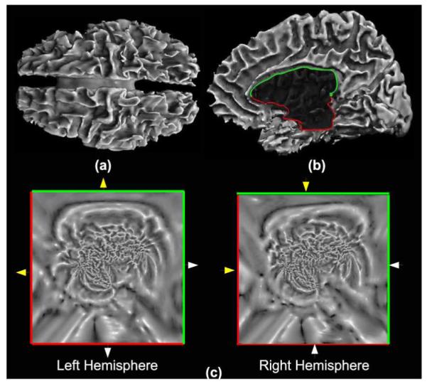
(a) Cortical surface extracted from MR data using the BrainSuite software. (b) Closed curve in the fissure between the two hemispheres divides the brain into two hemispheres; this curve is constrained to lie on the boundary of the unit square for both hemispheres. (c) 2-D coordinate system resulting from the p-harmonic mapping of the cortical surface. The mean curvature of the cortical surface is shown as a scalar image in this 2-D space. The arrows indicate connectivity along the boundary of the square between the two hemispheres, which is used for computing numerical approximations of the partial derivatives along this boundary.

For discretization of the anisotropic diffusion operator from (7), we compute the conduction function D(s, t) using (9) and arrange it in a column, denoted by D.

Then the isotropic and anisotropic diffusion operators are given by

$$L=G^I\left(D_{u^1}^f{D}_{u^2}^f\right)G^{r}G\left(\begin{array}{c}\hfill D_{u^1}^f\hfill \\ \hfill D_{u^2}^f\hfill \end{array}\right)$$ (23)

$$L^a=G^I\left(D_{u^1}^f{D}_{u^2}^f\right)D^{r}G\left(\begin{array}{c}\hfill D_{u^1}^f\hfill \\ \hfill D_{u^2}^f\hfill \end{array}\right)$$ (24)

where

$$G^I=\mathrm{diag}(1∕\sqrt{g}),$$ (25)

$$D^r=\mathrm{diag}\left([D,D][\sqrt{g},\sqrt{g}]\right)$$ (26)

$$G^r=\mathrm{diag}\left([\sqrt{g},\sqrt{g}]\right)\text{and}$$ (27)

$$G=\left(\begin{array}{cc}\hfill \mathrm{diag}\left(g^{11}\right)\hfill & \hfill \mathrm{diag}\left(g^{12}\right)\hfill \\ \hfill \mathrm{diag}\left(g^{12}\right)\hfill & \hfill \mathit{diag}\left(g^{22}\right)\hfill \end{array}\right).$$ (28)

In the discretization, we use forward and backward difference operators alternately in order to keep the numerical template of derivatives small [16].

The discretization of the isotropic and anisotropic operators is carried out in the following steps.

1. Parameterize the cortical surface to map it in two squares and assign it the coordinate system described in the Appendix.

2. Form the forward and backward difference matrices $D_{u^1}^f$, $D_{u^2}^f$, $D_{u^1}^b$, $D_{u^2}^b$, and for u¹ and u² coordinates, respectively, according to (19)-(22).

3. Compute the surface metric coefficients g, g₁₁, g₁₂, g₂₁ and g₂₂ and also the inverse metric coefficients g¹¹, g¹², g²². This is done by replacing partial derivatives in (15), (16), (17), (18) by their discrete versions from step 2.

4. Compute the isotropic or anisotropic Laplace-Beltrami operators using (23) or (24), respectively. For the anisotropic diffusion operator (11), we use the conduction function given by (9), with coefficient χ = 0.1. This value was chosen empirically.

In the case of isotropic diffusion, discretization of the diffusion operator needs to be carried out only once before starting the time iterations. On the other hand, for anisotropic diffusion the diffusion operator depends on I(s, t) and, hence, needs to be updated by carrying out the last step 4 repeatedly after every time step. In order to decrease this numerical cost, we update the operator after every 100 iterations assuming that the incremental change in I(s, n) is small.

The impulse response of the isotropic diffusion filter is shown in Fig. 2 both on the cortical surface and in the parameter space of one hemisphere. It can be seen that use of the surface metric results in an impulse response on the cortical surface with a greater degree of circular symmetry. Note that because of the nonlinear nature of the anisotropic diffusion filter, its behavior cannot be fully characterized by its impulse response.

Fig. 2.

Figure depicts the importance of using metric coefficients in (2). (a) The impulse response of the isotropic smoothing filter computed by solving the diffusion equation directly with respect to the 2-D coordinates without using metric coefficients. Note that the kernel is radially symmetric in the flat space but not symmetric when mapped back to the cortical surface. (b) In this case, we generate the isotropic smoothing kernel with respect to the intrinsic geometry of the cortical surface. In this case, the kernel appears highly nonsymmetric in the flat space, but becomes symmetric when mapped back to the cortical surface. (a) The heat kernel computed using the Laplacian in the (u, v) parameter space. (b) The heat kernel computed using the Laplace-Beltrami operator on the cortical surface.

IV. Results

We performed numerical studies on an Intel Pentium 4, 3.2-GHz computer with 2 GB of RAM using MATLAB. The cortical surface was extracted from a 256 × 256 × 170 voxel T1-weighted brain MR image of a volunteer subject. Processing time from the raw MR volume to extraction of the topologically corrected and tessellated cortex using BrainSuite took 7 min. The tessellated cortex had a total of 1.4 million nodes. The p harmonic parameterization of the 1.4 million node cortical surface with p = 4 took 37 s. Adding the parameterization step does not add significantly to the total computational cost compared to a direct FEM method [13], [12]. The number of iterations n along with the size of the time step δ determines the amount of smoothing applied. Smaller values of δ result in more numerically accurate solutions while the execution time is directly proportional to n. We chose δ = 1 × 10^-5 and n = 40000. Isotropic diffusion on the resampled surface took 20 min with this choice of n and δ while anisotropic diffusion took 1.5 h. The difference in execution times is mainly due to the nonlinear nature of the anisotropic diffusion which requires recomputation of the diffusion operator L repeatedly during the iterations. The code through parameterization was implemented in C/C++ with substantial effort directed at optimizing run-times while the diffusions were computed in MATLAB and, based on our earlier experience, we can expect a several-fold speed up when these are reprogrammed directly in C/C++.

In order to validate the method for isotropic diffusion, we compute the impulse response K_t(p, q) of the diffusion operator (heat-kernel) on a unit sphere. The heat-kernel K_t(p, q) is defined as the solution to the initial value problem

$$K_0(p,q)=\delta (p,q)$$ (29)

$$\frac{\partial K_t(p,q)}{\partial t}=\Delta K_t(p,q).$$ (30)

The heat-kernel on the unit sphere has a closed form analytical expression [26] given by

$$K_t(p,q)=\sum _{l=0}^{\infty }\frac{2l+1}{4\pi }{e}^{-l(l+1)t}{P}_l^0(p\cdot q)$$ (31)

where p is the starting point of the impulse and q is the point where measurement of the impulse response is made. In this case, the amount of spread is governed by time t in the diffusion (1). $P_l^0$ are the Legendre polynomials. The impulse response for different values of t is plotted on the unit sphere in Fig. 3. We also calculated the heat kernel using the diffusion filter defined in Section II-A and compared its accuracy with the analytically computed filter. We used a triangulated mesh with 300 000 vertices to represent the unit sphere. Each hemisphere was mapped to a unit square by (x, y, z) ↦ (sign(x)x² + sign(y)y², sign(x)x² - sign(y)y²). This parameterization was used for the numerical discretization of the Laplace-Beltrami operator in (1).

Fig. 3.

Heat-kernel on the unit sphere computed using the analytical expression as well as the parameterization based numerical method for t = 0.1 (b) t = 0.5 and (c) t = 1. The top row shows the heat-kernel computed analytically on the sphere. The second and third rows show numerically computed kernel on the sphere and in the flat paramater space. The two squares are maps of the upper and lower hemispheres, with the square boundary corresponding to a great circle around the equator of the sphere.

The root mean square percentage error compared to the analytical expression for t = 0.1, 0.5 and 1 was 2.31, 2.1 and 1.32, respectively. The errors are relatively small and do not appear to increase with time. Note that since the metric distortion is accounted for in the computation of the Laplace-Beltrami operator, the errors result from resampling and discretization of the parameterized surface and numerical approximation of derivatives. In order to study the behavior of the numerical errors in our method, we compared the percentage error in the numerically computed heat-kernel for different step sizes and grid sizes. As shown in Fig. 4, we can see that this error is a monotonically decreasing function of grid size and a monotonically increasing function of step size.

Fig. 4.

Percentage error in the numerically computed heat kernel on the sphere as a function of (a) grid size with fixed step size δ = 1 × 10^-6 and (b) step size for fixed grid of size 256 × 256.

We also applied the diffusion operators to mean curvature maps computed on the cortical surface. We compute the mean curvature using the method described in [27] and resample it on the regular grid. However, we note that an added advantage of our approach is that we can also compute the mean curvature by using our discretization of the metric tensor. In particular, the mean curvature H can be computed as

$$H=\frac{1}{2}{b}_{\alpha \beta }{g}^{\alpha \beta }$$ (32)

where the second fundamental form b_αβ is given by

$$b_{\alpha \beta }=\frac{1}{\sqrt{g}}\left[\frac{\partial \mathbf{x}}{\partial u^1}+\frac{\partial \mathbf{x}}{\partial u^2}+\frac{{\partial }^2\mathbf{x}}{\partial u^{\alpha }\partial u^{\beta }}\right].$$ (33)

The minima and saddle points of the mean curvature of the cortical surface are known to follow the sulcal patterns [27] and, therefore, are vital features for automatic labeling of the sulci [28]. However, as can be seen in Fig. 5(a), there is a considerable amount of noise in the mean curvature computed on the cortical surface. This is primarily due to the fact that the mean curvature is a local feature and is, therefore, prone to errors in extraction and discretization of the cortical surface. We see that the isotropic diffusion filtering smoothes out this noise, but since this filtering is not region selective, it also blurs the regions between sulci (positive mean curvature) and gyri (negative mean curvature) as seen in Fig. 5(b). On the other hand, anisotropic filtering removes noise while carrying out the smoothing only within regions and, thus, respects boundaries between sulci and gyri as seen in Fig. 5(c), thus illustrating the advantage of anisotropic filtering.

Fig. 5.

Left: Mean curvature of the cortical surface plotted on a smoothed representation for improved visualization of curvature in sulcal folds; right: the mean curvature plotted in 2-D parameter space for a single cortical hemisphere. (a) Shows the mean curvature maps on the surface and in the flat space for one hemisphere. (b) Isotropic diffusion filtering smoothes uniformly on the cortical surface, thus losing detail in the curvature map, while (c) anisotropic diffusion filtering removes the fine grain noise structure, while retaining the larger scale details in the curvature map. (a) Locally computed (noisy) mean curvature. (b) Isotropically smoothed mean curvature. (c) Anisotropically smoothed mean curvature.

V. Discussion

We have described a computational procedure for diffusion filtering of scalar images defined on nonflat surfaces. Using a parameterized representation of the surface, we compute a solution to the diffusion equation in which metric tensors are used to account for the curvature of the surface and intrinsic distances. The resulting diffusions are computed with respect to the intrinsic geometry of the surface and are, therefore, independent of the specific parameterization used, so long as the parameterization is fine enough. We also presented a Crank-Nicolson type scheme for discretization of the time derivative in order to make these filters stable. Our parameterization-based method can be used for both isotropic and anisotropic diffusion smoothing, as we demonstrated by performing these operations to mean curvature maps on models of the cerebral cortex. The resulting computational procedures are relatively efficient and stable, requiring approximately 30 min of computation for isotropic smoothing on a single cortex, including the preprocessing time necessary to extract the parameterized representation of the cortical surface.

In the context of neuroimaging, isotropic forms of diffusion described here may be used for spatially invariant smoothing of anatomical, functional or statistical data on the cortical surfaces in situations where selective smoothing is not required. Applications include filtering of functional data when smoothness is required for application of parametric random-field methods for control of false positives in multiple hypothesis testing [29].

Anisotropic diffusion filtering can be used for applications where region selective smoothing is advantageous, such as for studying gyrification of the cortex by mean curvature maps [30]-[32]. In functional studies involving different visual tasks, it may be advantageous to discourage smoothing across different visual areas [33]. These techniques can also be used for multiscale representations of functional activation [4], statistical data [5], and neuro-anatomical variability [3]. Surface matching across subjects may also be implemented using covariant PDEs, which essentially compute flows that are regular with respect to the surface metric, and are invariant to smooth changes in coordinates [3], [4]. In these flows, it is also necessary to compute the Laplace-Beltrami operators of a vector field, and it is also possible, by analogy, to regularize higher order tensor fields using a manifold-derived metric (e.g., for enhancing diffusion tensor images).

Appendix

In order to solve the smoothing equations on the cortical surface, a p-harmonic parameterization described in [25] is used. The 2-D coordinate system generated by this parameterization is used for the discretizations as described in Section III. Note that since the metric associated with the coordinate system is included in the computations, any other flattening method can be used instead of these mappings. In this Appendix, we briefly describe our p-harmonic parameterization scheme.

Let $\overrightarrow{u}=(u^1,u^2)$ be a function defined on a surface S such that $\overrightarrow{u}:S\mapsto R^2$. The p-harmonic energy functional is defined as the surface integral

$${\int }_S{\mid \nabla \overrightarrow{u}\mid }^{p}dS.$$ (34)

The p-harmonic maps are the minimizers of this energy. The existence, uniqueness, and other properties of these maps have been studied [36]-[38]. We use these maps to flatten the two brain hemispheres to two unit squares. The cortical surface model extracted using BrainSuite is represented as a high resolution triangulated mesh with around 1 million vertices. The corpus callosum which divides the two cortical hemispheres is identified as a closed contour in the cortical mesh. This contour is then constrained to lie on the unit square. With this as the mapping constraint, the p-harmonic energy minimization leads to a system of linear equations with a sparse system matrix as explained in [25]. Here we present the discretization formulae for completeness and ease of implementation. The detailed derivation is presented in [25].

We assume that the mapping function $\overrightarrow{u}$ is piecewise linear over the surface, i.e., it is linear over each triangle. For such functions, the gradient operator for ith triangle is given by

$$\begin{array}{cc}\hfill \overrightarrow{\nabla }& =\frac{1}{2A^i}\underset{B^i}{\overset{\left[\begin{array}{ccc}\hfill y_2^i-y_1^i\hfill & \hfill y_3^i-y_1^i\hfill & \hfill y_1^i-y_2^i\hfill \\ \hfill x_1^i-x_2^i\hfill & \hfill x_1^i-x_3^i\hfill & \hfill x_2^i-x_1^i\hfill \end{array}\right]}{\underbrace{}}}\hfill \\ \hfill & =\frac{1}{2A^i}{B}^i\hfill \end{array}$$

where Aⁱ is the area of triangle i and $x_k^i$, $y_k^i$, $z_k^i$ denote the x, y, z coordinates of the kth vertex of ith triangle. Since $\overrightarrow{u}$ is piecewise linear, its gradient is constant over each triangle i, so that

$$\int \mid \mid \nabla \overrightarrow{u}\mid \mid dS=\sum _i{\mid \mid \nabla \overrightarrow{u}\mid \mid }^p{A}^i$$

where the sum is over all triangles. The energy minimization discretizes to

$$\underset{\overrightarrow{u}}{\arg \min }\int {\mid \mid \nabla \overrightarrow{u}\mid \mid }^{p}dS=\underset{\overrightarrow{u}}{\arg \min }\sum _i{\Vert \frac{1}{2^p{\left(A^i\right)}^{p-1}}{B}^i{\overrightarrow{u}}^i\Vert }^p$$

where ${\overrightarrow{u}}^i$ are the values of the map $\overrightarrow{u}$ on the ith triangle. This energy discretization with the unit square mapping constraint on the vertices corresponding to corpus callosum is solved using a preconditioned conjugate-gradient minimization method resulting in the p-harmonic maps shown in Fig. 1. We use a Jacobi preconditioner for the minimization. The mapping function is integrated into our BrainSuite package [22] and is available for download at http://brainsuite.usc.edu.

References

- [1].Romeny B. Geometry-Driven Diffusion in Computer Vision. Kluwer; Norwell, MA: 1994. [Google Scholar]
- [2].Thompson P, Toga A. A surface-based technique for warping three-dimensional images ofthe brain. IEEE Trans. Med. Imag. 1996 Apr;15(4):402–417. doi: 10.1109/42.511745. [DOI] [PubMed] [Google Scholar]
- [3].Thompson PM, et al. Dynamics of gray matter loss in Alzheimer’s disease. J. Neuroscience. 2003;23(3):994–1005. doi: 10.1523/JNEUROSCI.23-03-00994.2003. [DOI] [PMC free article] [PubMed] [Google Scholar]
- [4].Joshi AA, Shattuck DW, Thompson PM, Leahy RM. A framework for registration, statistical characterization and classification of cortically constrained functional imaging data; Proc. Lecture Notes in Computer Science; Jul. 2005; pp. 186–196. [DOI] [PMC free article] [PubMed] [Google Scholar]
- [5].Chung MK, Robbins SM, Dalton KM, Davidson RJ, Alexander AL, Evans A. Cortical thickness analysis in autism with heat kernel smoothing. Neurolmage. 2005 May;25(4):1256–1265. doi: 10.1016/j.neuroimage.2004.12.052. [DOI] [PubMed] [Google Scholar]
- [6].Hagler DJ, Jr., Saygin AP, Sereno MI. Smoothing and cluster thresholding for cortical surface-based group analysis of fMRI data. NeuroImage. 2006 Dec;33(4):1093–1103. doi: 10.1016/j.neuroimage.2006.07.036. [DOI] [PMC free article] [PubMed] [Google Scholar]
- [7].Chung MK, et al. Diffusion smoothing on the cortical surface. NeuroImage. 2001 June;13(6S1):95. [Google Scholar]
- [8].Chung MK. Introducing heat and geodesic kernel smoothing on cortical manifolds; presented at the 11th Annu. Meet; OHBM, Toronto, ON, Canada. 2005. [Google Scholar]
- [9].Perona P, Malik J. Scale-space and edge detection using anisotropic diffusion. IEEE Trans. Pattern Anal. Mach. Intell. 1990 Jul;PAMI-12(7):629–639. [Google Scholar]
- [10].Hildebrandt K, Polthier K. Anisotropic filtering of non-linear surface features. Comput. Graph. Forum. 2004 Sept;23(3):391–400. [Google Scholar]
- [11].Clarenz U, Diewald U, Rumpf M. Processing textured surfaces via anisotropic geometric diffusion. IEEE Trans. Image Process. 2004 Feb;13(2):248–261. doi: 10.1109/tip.2003.819863. [DOI] [PubMed] [Google Scholar]
- [12].Lopez-Perez L, Deriche R, Sochen N. The Beltrami flow over triangulated manifolds; Proc. ECCV Workshops CVAMIA and MMBIA; 2004.pp. 135–144. [Google Scholar]
- [13].Bajaj C, Xu G. Anisotropic diffusion of surfaces and functions on surfaces. ACM Trans. Graphics (TOG) 2003;22(1):4–32. [Google Scholar]
- [14].Andrade A, Kherif R, Mangin J, Worsley K, Paradis A, Simon O, Dehaene S, Bihan DL, Poline J. Detection of fMRI activation using cortical surface mapping. Human Brain Map. 2001;12:79–93. doi: 10.1002/1097-0193(200102)12:2<79::AID-HBM1005>3.0.CO;2-I. [DOI] [PMC free article] [PubMed] [Google Scholar]
- [15].Qiu A, Bitouk D, Miller M. Smooth functional and structural maps on the neocortex via orthonormal bases of the Laplace-Beltrami operator. IEEE Trans. Med. Imag. 2006 Oct;25(10):1296–1306. doi: 10.1109/tmi.2006.882143. [DOI] [PubMed] [Google Scholar]
- [16].Smith GD. Numerical Solution of Partial Differential Equations: Finite Difference Methods, ser. Oxford Applied Mathematics and Computing Science. 3rd ed. Clarendon; Oxford, U.K.: 1985. [Google Scholar]
- [17].Bertalmio M, Cheng L-T, Osher S, Sapiro G. Variational Problems and Partial Differential Equations on Implicit Surfaces: The Framework and Examples in Image Processing and Pattern Formation, Tech. Rep. Univ. California; Los Angeles: Jun, 2000. [Google Scholar]
- [18].Mémoli F, Sapiro G, Osher S. Solving variational problems and partial differential equations mapping into general target manifolds. J. Comput. Phys. 2004;195(1):263–292. [Google Scholar]
- [19].Mémoli F, Sapiro G, Thompson P. Implicit brain imaging. Neuroimage: Mathematics in Brain Imaging. 2004;23(Supp 1):S179–S188. doi: 10.1016/j.neuroimage.2004.07.072. [DOI] [PubMed] [Google Scholar]
- [20].Kreyzig I. Differential Geometry. Dover; New York: 1999. [Google Scholar]
- [21].Sochen N, Deriche R, Perez-Lopez L. Variational Beltrami flow over implicit manifolds; presented at the Int. Conf. Image Processing; Barcelona, Spain. 2003. [Google Scholar]
- [22].Shattuck DW, Leahy RM. Brainsuite: An automated cortical surface identification tool. Med. Image Anal. 2002;8(2):129–142. doi: 10.1016/s1361-8415(02)00054-3. [DOI] [PubMed] [Google Scholar]
- [23].Shattuck DW, Sandor-Leahy SR, Schaper KA, R DA, Leahy RM. Magnetic resonance image tissue classification using a partial volume model. NeuroImage. 2001 May;13(5):856–876. doi: 10.1006/nimg.2000.0730. [DOI] [PubMed] [Google Scholar]
- [24].Shattuck DW, Leahy RM. Automated graph-based analysis and correction of cortical volume topology. IEEE Trans. Med. Imag. 2001 Nov;20(11):1167–1177. doi: 10.1109/42.963819. [DOI] [PubMed] [Google Scholar]
- [25].Joshi AA, Leahy RM, Thompson PM, Shattuck DW. Cortical surface parameterization by p-harmonic energy minimization; Proc. IEEE Int. Symp. Biomedical Imaging; 2004; pp. 428–431. [DOI] [PMC free article] [PubMed] [Google Scholar]
- [26].Chung MK. Heat kernel smoothing on unit sphere; presented at the IEEE Int. Symp. Biomedical Imaging; 2006. [Google Scholar]
- [27].Cachia A, et al. A primal sketch of the cortex mean curvature: A morphogenesis based approach to study the variability of the folding patterns. IEEE Trans. Med. Imag. 2003 Jun;22(6):754–765. doi: 10.1109/TMI.2003.814781. [DOI] [PubMed] [Google Scholar]
- [28].Rettmann M, Han X, Xu C, Prince J. Automated sulcal segmentation using watersheds on the cortical surface. NeuroImage. 2002;15(2):329–344. doi: 10.1006/nimg.2001.0975. [DOI] [PubMed] [Google Scholar]
- [29].Worsley K, Marrett S, Neelin P, Vandal A, Friston K, Evans A. A unified statistical approach for determining significant signals in images of cerebral activation. Human Brain Map. 1996;4:58–73. doi: 10.1002/(SICI)1097-0193(1996)4:1<58::AID-HBM4>3.0.CO;2-O. [DOI] [PubMed] [Google Scholar]
- [30].Luders E, Thompson P, Narr K, Toga A, Jancke L, Gaser C. A curvature-based approach to estimate local gyrification on the cortical surface. NeuroImage. 2006 Feb;29(4):1224–1230. doi: 10.1016/j.neuroimage.2005.08.049. [DOI] [PubMed] [Google Scholar]
- [31].Gaser C, Luders E, Thompson PM, Lee AD, Dutton RA, Geaga JA, Hayashi KM, Bellugi U, Galaburda AM, Korenberg JR, Mills DL, Toga AW, Reiss AL. Increased local gyrification mapped in Williams syndrome. NeuroImage. 2006 Oct;33(1):46–54. doi: 10.1016/j.neuroimage.2006.06.018. [DOI] [PubMed] [Google Scholar]
- [32].Lui LM, Wang YL, Chan TF, Thompson PM. Brain anatomical feature detection by solving partial differential equations on a general manifold. J. Discrete Continuous Dyn. Syst. B. 2007 May;7(3):605–618. [Google Scholar]
- [33].Calhoun VD, Adali T, McGinty VB, Pekar JJ, Watson TD, Pearlson GD. fMRI activation in a visual-perception task: Network of areas detected using the general linear model and independent components analysis. NeuroImage. 2001;14(5):1080–1088. doi: 10.1006/nimg.2001.0921. [DOI] [PubMed] [Google Scholar]
- [34].Tang B, Sapiro G, Caselles V. Diffusion of general data on non-flat manifolds via harmonic maps theory: The direction diffusion case. Int. J. Comput. Vis. 2000;36(2):149–161. [Google Scholar]
- [35].Chung MK, Qiu A, Nacewicz BM, Dalton KM, Pollak S, Davidson RJ. Tiling manifolds with orthonormal basis; presented at the 2nd MICCAI Workshop on Mathematical Foundations of Computational Anatomy (MFCA); 2008. [Google Scholar]
- [36].Xin Y. Geometry of Harmonic Maps. Birkhäuser; New York: 1996. [Google Scholar]
- [37].Fardoun A, Regbaoui R. Heat flow for p-harmonic maps between compact Riemannian manifolds. Indiana Univ. Math. J. 2002;51:1305–1320. [Google Scholar]
- [38].Hamilton R. Lecture Notes in Mathematics, ser. 471. Springer; New York: 1975. Harmonic maps of manifolds with boundary. [Google Scholar]