

Abstract
Sulcal and gyral landmarks on the human cerebral cortex are required for various studies of the human brain. Whether used directly to examine sulcal geometry, or indirectly to drive cortical surface registration methods, the accuracy of these landmarks is essential. While several methods have been developed to automatically identify sulci and gyri, their accuracy may be insufficient for certain neuroanatomical studies. We describe a semi-automated procedure that delineates a sulcus or gyrus given a limited number of user-selected points. The method uses a graph theory approach to identify the lowest-cost path between the points, where the cost is a combination of local curvature features and the distance between vertices on the surface representation. We implemented the algorithm in an interface that guides the user through a cortical surface delineation protocol, and we incorporated this tool into our BrainSuite software. We performed a study to compare the results produced using our method with results produced using Display, a popular tool that has been used extensively for manual delineation of sulcal landmarks. Six raters were trained on the delineation protocol. They performed delineations on 12 brains using both software packages. We performed a statistical analysis of 3 aspects of the delineation task: time required to delineate the surface, registration accuracy achieved compared to an expert-delineated gold-standard, and variation among raters. Our new method was shown to be faster to use, to provide reduced inter-rater variability, and to provide results that were at least as accurate as those produced using Display.
Keywords: Cerebral cortex, Sulci, Delineation, Landmarks, Surface registration
1. Introduction
The examination of the patterns of variation in the human brain often relies upon the accurate identification of structures on the surface of the cerebral cortex. Sulci are of great interest in the structural analysis of magnetic resonance imaging (MRI), where the functional and architectonic boundaries are not directly visible. These boundaries have been linked to various characteristics of the sulci (Watson et al., 1993; Roland and Zilles, 1994), thus major functional areas in the brain may be associated with sulci. Similarly, various gyri have been associated with a variety of brain functions. Fischl et al. (2007) have recently reported that localization of Broadman areas with respect to folding patterns demonstrates stability, providing further motivation for aligning cortical data based on geometric structure.
There are a number of sulci that appear reliably in normal brains; however, these structures are characterized by large variations across subjects (Ono et al., 1990). These variations have been studied in relationship to several aspects of health and disease. Early studies of sulci using MRI relied upon tracings on images with slice thicknesses of 5-9 mm (Missir et al., 1989; Steinmetz et al., 1989, 1990). Kikinis et al. (1994) traced sulcal patterns in 2D on renderings made from 3D images of brains oriented to the same camera view. Thompson et al. (1996) performed statistical analysis of high-resolution 3D sulcal curves that were traced on human cryosection data. These techniques were later extended and applied to MRI in several studies that examined sulcal asymmetry in the hemispheres. These included explorations of the brain during developmental stages (Blanton et al., 2001; Sowell et al., 2002), in subjects with schizophrenia (Narr et al., 2001), and in relationship to handedness and gender (Luders et al., 2003).
Since the sulci typically separate the brain into distinct functional areas, spatial normalization techniques have been developed that use explicitly defined sulcal features as constraints. Thompson et al. (1997) computed high-dimensional volumetric maps by elastically deforming scans into structural correspondence using landmarks that were traced manually on the cortical surface. Collins et al. (1998) combined sulcal ribbons with image-based features for volumetric registration. Cachier et al. (2001) used automatic sulcal identification and labeling followed by a combination of linear point matching and intensity matching to achieve intersubject correspondence. Joshi et al. (2007) used sulcal landmarks as constraints in a combined surface parameterization/registration approach, which was extended to the whole volume by constrained harmonic mapping, and finally refined using an intensity-based warp. Surface-based registration techniques, such as those described by Davatzikos et al. (1996), Fischl et al. (1999), or Tosun and Prince (2005), may also be used to align cortical surface models based on geometric features of the surface without the use of explicit constraints. These aligned maps can then be used to study the properties of the cortex in sulcal or gyral regions. Fischl et al. (2004) developed a method for labeling each point on the surface with a neuroanatomical label based on a manually labeled training set and geometric priors. Yeo et al. (2008) extended this work, proposing a generative model for the joint registration and parcellation of the cortical surface that provided improved parcellation accuracy. Geometric features can also be combined with explicitly defined sulcal constraints (Eckstein et al., 2007).
Manual delineation of sulcal anatomy can be a time-consuming process, and much effort has gone into the development of automated approaches to identify sulci. We summarize a few of the recent methods here. Khaneja et al. (1998) applied dynamic programming to identify length minimizing geodesics and curves of extremal curvature to identify the sulcal fissures. Le Goualher et al. (1999) developed a method called sulcal extraction and assisted labeling (SEAL), which detected cortical ribbons that were then associated manually with known sulci. Zeng et al. (1999) developed an automatic intrasulcal ribbon finding technique using the distance function computed as part of a coupled level set surface extraction method. Caunce and Taylor (2001) applied active shape models to identify sulci. Tao et al. (2002) applied a statistical shape model to identify sulci on cortical surfaces that were mapped to the unit sphere. Rivière et al. (2002) generated maps of the cortical sulci using a graph matching approach based on neural networks trained with manually labeled data. Rettmann et al. (2002) applied a watershed method to the sulcal beds in order to identify major sulci; this was later augmented with a system to perform assisted labeling of the identified regions (Rettmann et al., 2005). Ratnanather et al. (2003) applied dynamic programming to identify crestlines on cortical surfaces. Tu et al. (2007) applied a supervised learning approach to perform extraction of sulcal lines from MRI using curves that were manually delineated.
While automated methods have been successfully applied in several settings, their accuracy may not be satisfactory for expert neuroanatomists, particularly in the presence of the wide variation that appears in neuroanatomy and in image acquisition quality. Data from subjects exhibiting abnormal cortical shape, such as individuals with Alzheimer’s disease, may be handled better by manual delineation. In registration applications, errors in automatic sulcal identification may propagate into errors in the registration accuracy. It is likely that landmarks defined by experts, who have been trained to make consistent decisions when faced with ambiguities that arise frequently in the analysis of cortical geometry, will produce improved registration results. In some cases a particular area, such as the visual cortex, may be of interest and constraints specific to that area may provide more appropriate registration. Furthermore, some of the methods for automatic sulcal delineation (e.g., Rivière et al., 2002; Tu et al., 2007) require an expert-labeled training set. Thus, in certain instances, it is still desirable to use a manual approach to perform sulcal landmark identification.
Several semi-automated methods have been developed that allow raters to define curves on the cortex. Display (Montreal Neurological Institute, Montreal, Canada) is an OpenGL-based software package that provides a 3D rendering of a cortical surface, synchronized with views of a corresponding MRI or other data. Users can define a series of points along a curve, which are joined using a shortest-path algorithm based on the Euclidean distance between edges on the surface mesh. The Caret software package (available online at http://brainmap.wustl.edu/caret/) provides facilities for delineation of landmarks on various types of neuroanatomical data, including inflated and flattened cortical surfaces (Van Essen et al., 2001). Sulcal landmarks produced with Caret have been used in surface-based registration processes (Van Essen, 2005). The RView software package (available online at http://rview.colinstudholme.net) displays volume and surface data; it also provides the capability to define sets of points joined by straight line segments to define landmarks such as sulci. Bartesaghi and Sapiro (2001) developed a system for optimally computing geodesics on surfaces, and used it to identify sulci and gyri based on local curvature measures. Hurdal et al. (2008) applied Dijkstra’s algorithm to find shortest paths between endpoints of sulci, using a weighted graph with an edge cost function designed to follow crestlines such as gyri or sulci. Studies of variation in manually delineated sulcal delineations can be limited by the variations in the definitions of the end points of sulcal curves, specifically when pointwise correspondence between curves is derived from the end point positions. To address this problem, Durrleman et al. (2008) proposed measuring the distance between landmark curves using currents, with no implicit assumption of pointwise correspondence.
In this paper, we describe a semi-automated curve tracking algorithm and its implementation as part of a curve tracing protocol software tool. The curve tracking method computes a weighted graph from the vertices and edges of a triangle mesh representation of the cerebral cortex. The weight of each edge is determined by a combination of local curvature features and the distance between vertices on the surface representation. Given two seed points on the surface, we use a shortest path algorithm on the weighted graph to determine a series of edges that follow the valleys of sulci or the ridges of gyri. The tracking tool was integrated into our existing BrainSuite software package (Shattuck and Leahy, 2002) to guide the user through the process of identifying a sequence of well-defined landmarks on the cortical surface. The user can seed multiple points along the path and view the results in real-time as points are added or as the end point of the curve is moved on the surface. The view of the curve traced on the cortical surface is synchronized with a view of orthogonal slices in a corresponding 3D image volume, providing the user with additional context for decision making during the delineation process. To establish performance relative to an established software tool, we performed inter-rater and intra-rater comparisons using both Display and our new BrainSuite tool. The results demonstrate that our new method can achieve comparable accuracy with reduced inter-rater variability in dramatically less time.
2. Methods
2.1. Curve-tracking procedure
We assume, as input to our algorithm, a triangular mesh M, comprising a set of vertices, V = {v1, v2, . . . , vNV}, and a set of edges, E = {e1, e2, . . . , eNE} that compose the triangles of the mesh. Each vertex vi ∈ V is a point in 3D space, and each edge ej ∈ E is a pair of integers corresponding to the indices of the vertices V. This triangle mesh can be produced in a number of ways. In this work, we focus our validation on surfaces produced by the method of MacDonald (1998), though we have also applied the technique to surfaces produced with our own BrainSuite software (Shattuck and Leahy, 2002), FreeSurfer (Dale et al., 1999), and BrainVoyager (Brain Innovation B.V., Maastricht, The Netherlands).
Given a pair of points va ∈ V and vb ∈ V, we compute an optimal path through a weighted graph constructed from the surface mesh. While we could define the weights of this graph using the Euclidean distances of the edges in the path, such a path would be unlikely to follow the neuroanatomical features of the surface. Instead, we compute the cost of each edge using the Euclidean distance modulated by a measure of the local convexity at each point. The path that is found will thus depend on the local properties of the surface.
2.1.1. Convexity measure
We define the convexity measure at each vertex index i as
| (1) |
where Ni is the set of first-order neighbors of vertex i, i.e., those vertices sharing an edge with vi, |Ni| is the size of set Ni, vi is the 3D spatial position of vertex i, and n̂i is the surface normal at i. The surface normal n̂i is computed as the average of the normals of the triangles adjacent to vertex vi, with the convention that the normals point outwards from the surface.
In simpler terms, the sum in Eq. (1) averages the cosines of the angles between the surface normal at vi and the edges connected to that vertex. Fig. 1 shows a map of the convexity measures for a cortical surface model. In a flat configuration, ci will be zero since the surface normal is orthogonal to the connected edges. If the surface is locally concave, i.e., has negative mean curvature, at that point, then the angles will be in the range (0, π/2) since all points in the neighborhood are above the tangent plane. Thus, the sum will be positive, and ci will be negative. Similarly, if the surface is locally convex, i.e., has positive mean curvature, then the sum will be negative and ci will be positive. In previous work, we adopted this measure (Timsari and Leahy, 2000) in place of mean curvature, as it could be computed rapidly. We note here that this measure could be replaced by more formal discrete approximations of curvature, such as those described by Meyer et al. (2003). In practice, the convexity measure we selected has been effective and produced sulcal tracking results that were satisfactory to neuroanatomists.
Fig. 1.
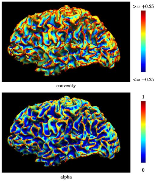
A cortical surface model shaded by (top) its convexity measure and (bottom) the cost function (α).
2.1.2. Graph weighting
We create a weighted graph G = (E, V, W) from the edge and vertex sets, E and V. The weighting wk ∈ W of an edge ek = (vi, vj), ek ∈ E is determined by the equation
| (2) |
where αi is a cost function that we define at each vertex
| (3) |
where ci is the local measure of convexity, κ is a global constant controlling the slope of the sigmoid, and λ is a second global constant that determines the influence of the convexity term in the weighting function. In this work, we use κ = 20 for the sigmoid slope. We did not perform extensive testing of this parameter, but this value demonstrated acceptable performance during initial development of the algorithm. The sigmoid provides a limit on extreme convexity measures, making the method more robust to rapid changes in the surface that result from noise that is often present in surface models, such as those produced from tissue classification maps. The weight averages the robust convexity measure along the edge. When λ = 0, the weighting is based solely on the Euclidean distance between the two vertices; when λ > 0, paths through convex regions will have higher costs than paths of equal edge length through concave regions, thus the path through the concave region will be preferred. Changing the sign of the convexity measure or the sign of κ will reverse this effect, allowing us to trace convex regions. In the context of cortical surface models, changing these parameters allows the algorithm to follow sulci or gyri when we apply this method to cortical surface models. Lambda is user-adjustable. We selected a default value of λ = 2 based on our initial use of the algorithm; we did not formally test the stability of this parameter. The influence of λ will vary depending on the smoothness of the particular surface and feature being traced. On rough surfaces, increasing to larger values will cause the curve to trace around surfaces bumps which may be attributable to noise rather than anatomy. Fig. 1 shows a map of the vertex cost function, αi, for a cortical surface model, with κ = 20 and λ = 2.0. The darker blue areas indicate the lowest cost vertices, and are largely restricted to the sulcal fundi. Fig. 2 shows examples of curves traced upon white matter/grey matter boundary surfaces produced by BrainSuite using parameter settings to follow sulci, gyri, or unweighted edge length.
Fig. 2.
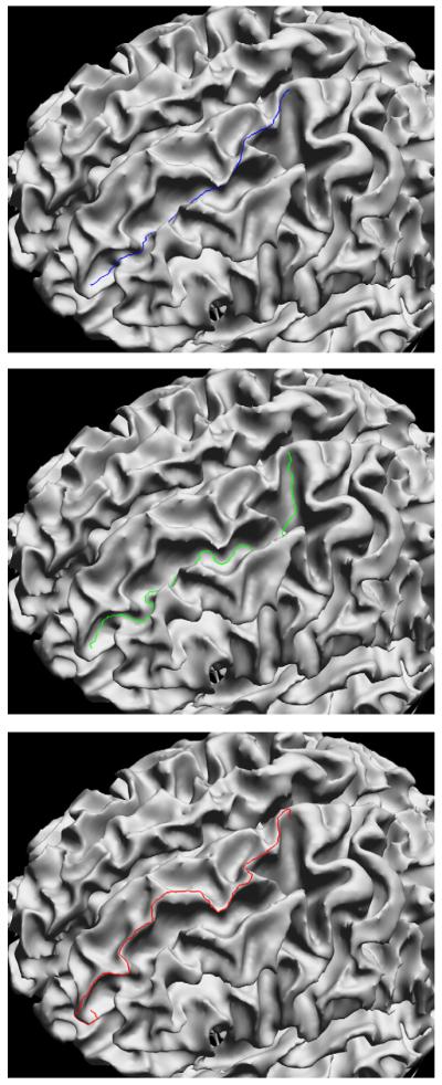
Surface curves traced with the method described in this paper; all points were traced using the same 2 seed points. (top) Surface curve automatically traced using the Euclidean distance along each edge (λ = 0). (middle) Sulcal curve traced using λ = 2 and positive convexity weighting. (middle) Gyral curve traced using λ = 2 and negative convexity weighting.
2.1.3. Path computation
Once the edge weighting has been determined, the graph can be used to compute paths between seed points. Given two vertices, va and vb, we compute the shortest weighted path between them using Dijkstra’s algorithm (Dijkstra, 1959). This path will be composed of contiguous points on the cortical surface mesh M, joined by edges from E. In practice, more complicated curves may be defined as the total path computed between adjacent pairs of points in an ordered set of points defined by the user.
2.2. Software implementation
2.2.1. Landmark identification
We built the curve identification algorithm into a customized version of our BrainSuite software (Shattuck and Leahy, 2002). BrainSuite uses OpenGL to display a 3D rendering of the cortical surface mesh (see Fig. 3). The user can interactively reorient this surface and zoom to different levels of detail. This view is synchronized with 3 orthogonal views of a corresponding 3D MRI volume that can be loaded into the interface. This allows the user to identify neuroanatomical landmarks through several views. The software can be run interactively on Windows-based PCs or on other platforms using tools such as WINE (http://www.winehq.org).
Fig. 3.

The BrainSuite curve protocol tool. Tracing protocols, defined in XML, can be loaded into the tool. The user can select a curve to be traced, and control the λ parameter, undo previous points selected, and save and load results. The interface also provides access to additional information via URLs encoded in the protocol specification.
When tracking a curve on the surface, the user can identify an initial seed point va by clicking on the view of the surface. The software then displays that point on the surface and computes the data used in the Dijkstra algorithm. This provides a fast method to compute the optimal path between va and any other point on the mesh. Once these data have been generated, the user can select a second point on the surface. The Curve Protocol software then generates the lowest cost path and displays it on the cortical surface model. Because all necessary data for optimal paths from va have been computed, the software updates the displayed curve as the user drags the next point to different locations on the surface. These updates occur in real-time on relatively modest personal computers; we have achieved acceptable performance on computers with 1.7 GHz Intel Pentium 4 processors. The rapid updates provide the user with direct feedback so that he or she can quickly select an appropriate endpoint or midpoint for a cortical landmark. This allows the user to ensure that the traced curve properly follows the anatomy, which would otherwise be difficult near interrupted sulci. Once an initial pair of points has been selected, the optimal path is displayed and the software computes the Dijkstra information from the second point. The user can then track curves from this next seed point, and this new path segment is added to the complete path. We also developed the software to provide undo features, allowing the user to rewind the curve to correct mistakes that may occur during the landmark selection process. The user can also adjust the parameter to determine the influence of the curvature weighting. For example, when tracing an interrupted sulcus, the user can cross another gyrus by setting the weighting to zero.
2.2.2. Protocol interface
Since the purpose of this software tool is to provide a mechanism for identifying a set of landmarks that are defined by a delineation protocol, we built a specialized interface that displays the protocol information within BrainSuite (see Fig. 3). A protocol file is specified using an XML document. This protocol file provides a definition for each curve, including descriptions of the start and stop points that should be used for the landmark, the direction in which the landmark curve, e.g., sulcus, should be traced, and additional notes of any features or special criteria that should be observed during the delineation process. An additional field is provided for a URL reference, which allows a webpage to be specified that provides additional information relating to the landmark.
When a user selects a curve in the curve protocol interface, BrainSuite displays the information for that curve and provides a button to launch the related webpage if required by the user. The user can trace curves defined by the protocol, save curve sets, and load them. The protocol is stored in the same file as the saved curves, thereby providing a record of which protocol was followed to define a set of landmarks. Each landmark can be described in the protocol as being required or optional, and BrainSuite will warn users when they save a set of curves that is incomplete. These curves can be exported in formats appropriate for surface registration methods (e.g., Thompson et al., 2004) or studies of sulcal variation (e.g., Blanton et al., 2001; Narr et al., 2001; Sowell et al., 2002; Luders et al., 2003). In this work, we adapted the existing LONI protocol (Sowell et al., 2002, protocol available online at http://www.loni.ucla.edu/Protocols/SulcalAnatomy) into this format. This protocol specifies each sulcal landmark to be traced by a single contiguous curve. Included in this protocol is the specification for how the rater should trace each landmark, including how to locate the landmarks on the brain surface and how to determine the path to take for each sulcus. The protocol accounts for many of the variations that are encountered across subjects; this provides a consistent set of rules that plays an important role in establishing reliable landmarks for intersubject analysis. For example, in the case of a bifurcation, the protocol specifies which path to follow. Similarly, in the case of a sulcus that may be interrupted by a gyrus, the protocol specifies how the traced curve should traverse the gyrus. In the case of tracing an interrupted sulcus with BrainSuite, the raters were instructed to adjust the curvature weighting to allow the curve tracker to cross gyri as necessary.
2.3. Validation methodology
To assess our new method, we compared its use to that of Display (Montreal Neurological Institute, Montreal, Canada), which had been used previously as a standard for delineation at the UCLA Laboratory of Neuro Imaging. Display allows users to delineate curves using an OpenGL interface, and it will compute paths along mesh edges between seed points using a shortest path algorithm.
Tracings were performed on 12 cortical surface meshes. These meshes were produced from T1-weighted MRI volumes using the cortical surface extraction method of MacDonald (1998). Each mesh represents one hemisphere of the brain. These surfaces were traced previously by experts within our laboratory to produce training standards for use within our laboratory; these expert delineations were performed using the Display software. The expert delineations included landmark curves on the lateral aspect of the brain hemisphere for six of these surfaces (L1-L6) and landmark curves on the medial aspect of the remaining six surfaces (M1-M6). A set of 23 curves (see Table 2) was selected that were determined to be consistently present in most subjects. Surfaces L1-L6 were used for evaluating 13 curves on the lateral surface of brains; surfaces M1-M6 were used for evaluating 10 curves on the medial surface. In principal, we could have evaluated the 23 curves on all 12 surfaces; however, we opted to use the existing expert delineations as our gold standard for evaluation since they have been used reliably for several years.
Table 2.
Inter-rater variance (in units of mm2) for protocol curves traced by 6 individuals using BrainSuite and Display
| Curve | BrainSuite | Display |
|---|---|---|
| Sylvian fissure | 0.0669 | 2.2214 |
| Central sulcus | 0.7552 | 1.4937 |
| Postcentral sulcus | 4.9397 | 5.2170 |
| Precentral sulcus | 0.4018 | 0.9754 |
| Superior temporal sulcus main body | 2.5692 | 1.7645 |
| Superior temporal sulcus ascending branch | 1.8983 | 1.7679 |
| Transverse occipital sulcus | 14.5701 | 14.1739 |
| Intraparietal sulcus | 1.5365 | 2.7808 |
| Primary intermediate sulcus | 1.7256 | 1.9433 |
| Inferior temporal sulcus | 0.6676 | 1.1129 |
| Inferior frontal sulcus | 0.7439 | 0.7983 |
| Superior frontal sulcus | 1.8302 | 4.1926 |
| Olfactory sulcus | 4.7014 | 5.4206 |
| Callosal sulcus | 0.7380 | 0.7472 |
| Superior rostral sulcus | 0.3383 | 0.6818 |
| Inferior rostral sulcus | 0.7287 | 1.0865 |
| Paracentral sulcus | 2.3139 | 2.8526 |
| Cingulate sulcus, anterior segment | 1.3430 | 2.8599 |
| Cingulate sulcus, posterior segment | 0.7920 | 2.5374 |
| Parieto-occipital sulcus | 3.1697 | 3.3113 |
| Calcarine sulcus, anterior segment | 0.7599 | 1.1439 |
| Calcarine sulcus, posterior segment | 3.1257 | 3.1236 |
| Subparietal sulcus | 1.5099 | 2.9581 |
Delineation of the surfaces was performed by six raters who had limited experience with cortical surface delineation and limited neuroanatomical knowledge. This selection of the raters should reduce bias effects that might otherwise result from experience with the delineation tools. We note that the raters were not blinded to which method they were using, as the tools have very different interfaces. The raters were trained on the LONI protocol by an experienced rater and trainer (E.K.). The raters delineated a set of 8 practice surfaces, constructed using the same methods as those used in the study. The raters had engineering backgrounds but minimal knowledge of brain anatomy. Therefore, training involved learning both cortical anatomy and the tracing protocol, as well as the use of the two software packages. Training sessions started with BrainSuite, because it provided better visualization of the cortical surfaces. A total of 6 cortical surfaces were traced by all participants, during which they familiarized themselves with cortical anatomy and the use of BrainSuite. A second tracing session then followed, during which the participants were instructed to trace 2 more surfaces with Display to learn how to use that software. Feedback on their delineation results was provided by the trainer.
The raters then delineated the 12 test cortical surface models. Each surface was delineated twice by each rater—once in Display and once in BrainSuite. The order in which the delineations were performed was randomized to reduce bias effects from fatigue and experience with the surfaces and software. Each rater was provided a schedule specifying which brain surface to trace with which software package. The lateral brain surfaces were traced first. In statistical terms, each rater was assigned the same 12 experimental units, produced by the combination of 2 software packages (BrainSuite,Display) × 6 brains(L1-L6). This order was randomized for each rater. The order was then repeated for the 6 medial surfaces, replacing L1 with M1, and so on. The raters were instructed to record the time taken to delineate each surface completely. A set of curves, which had previously been established by very experienced raters at the UCLA Laboratory of Neuro Imaging using the Display software tool, was used as the ground truth for this study. To compare BrainSuite and Display, we analyzed 3 aspects of the delineation task: time efficiency, delineation accuracy, and inter-rater variability.
2.3.1. Time efficiency
To analyze the delineation time, we considered the rater as a random factor, and the software (BrainSuite/Display) and delineation side (lateral/medial) as fixed factors. We followed the summary statistic approach and modeled the delineation time separately for each rater using an ANCOVA (analysis of covariance) design:
| (4) |
where ti is the delineation time for the ith cortical surface; si is the software indicator variable (0 for BrainSuite, 1 for Display); vi is the view indicator variable (0 for lateral, 1 for medial), hi is the habituation covariate, which denotes the brain delineation order (1 for the first brain, 2 for the second, etc.), and ei is the error term. Variables b1, b2, b3, and b4 are the estimable model parameters, and the first term b1 is the intercept term (mean delineation time). We use the superscript r to denote that the same model is fit separately per rater r. We include the view indicator in this model since brains L1-L6 were traced on the lateral side and brains M1-M6 were traced on the medial side. The medial and lateral tracing tasks differed significantly in key areas, including the numbers of curves traced, the difficulty in visualizing the anatomy, and the nature of the curves that were traced.
2.3.2. Delineation accuracy
Because of limited neuroanatomical knowledge, the raters often produced large tracing errors irrespective of software. Such erroneous tracings constitute large measurement outliers, which deemed the analysis of variance approach inaccurate. To evaluate whether delineation accuracy is affected by each software, we used the median statistic, which is robust to the presence of outliers.
For a surface s and a specified curve n, we estimate the error difference between Display and BrainSuite in a traced curve from a rater r as
| (5) |
where is the gold standard curve and e1 is a distance measure defined by
| (6) |
where the first term in (6) is the average minimum distance of each point in curve Da to a point in curve Db, and the second term is the average minimum distance from each point in Db to a point in Da. We note that this is one of the 24 distance measures based on the Hausdorff distance that were described by Dubuisson and Jain (1994). For each rater, we estimate the median of the error difference as
| (7) |
.
2.3.3. Inter-rater variability
To trace a curve, Display requires the selection of multiple points on a surface, which are then joined by line segments computed using the shortest path along the surface mesh edges. BrainSuite, on the other hand, guides curves based on a curvature weighted lowest-cost path algorithm. Therefore, as long as brain anatomy has been identified accurately, the software will tend to trace the same curve, reducing inter-rater variability. To evaluate this effect, we measured the inter-rater variance for each curve using the following equation:
| (8) |
where R = 6 is the number of raters.
3. Results
The 6 raters delineated all 12 brains according to the methods described above. In one case, due to a file transfer error, one rater had to retrace a single curve that had been traced in Display; the corrected file was used in this study. We assumed this had a minimal impact on the assessment of the methods and did not take this into account in the analysis. The raters did not record how many manually selected points were needed for each curve. The raters reported that they did not alter the default parameter settings (λ = 2.0) in the BrainSuite tracing tool, except in the case of interrupted sulci where they turned this feature off (λ = 0.0) in some instances. The raters did not have control over the value of κ, which was set to 20 in all cases.
3.1. Time performance
The estimated model for the time analysis ANCOVA model parameters bi for each rater are shown in Table 1. The b1 term indicates the mean time, in minutes, required to delineate a set of curves on a brain surface. The remaining terms indicate, for each rater, the differences in time required with respect to different aspects of the study. We note that the signs of each of these terms were consistent across the raters. The b2 term indicates the difference in time required to use Display instead of BrainSuite. The sign for b2 was positive for all raters, thus more time was needed to trace curves with Display. The time difference between tracing the medial surface, which requires fewer curves, and tracing the lateral surface is denoted by b3; its negative value indicates that the medial side was traced faster then the lateral. Finally, the habituation parameter b4 indicates that there was a linear learning effect, since its negative value indicates that less time was required to trace the latter brains in the set.
Table 1.
Estimated model parameters for each rater for the delineation time ANCOVA model, in units of minutes
| Parameter | Rater 1 | Rater 2 | Rater 3 | Rater 4 | Rater 5 | Rater 6 | |
|---|---|---|---|---|---|---|---|
| Mean delineation time | b1 | 16.0920 | 36.8500 | 12.2333 | 20.0667 | 19.2167 | 9.6667 |
| Software (BrainSuite/Display) | b2 | 15.2397 | 5.3333 | 6.8333 | 18.0833 | 11.4167 | 7.7500 |
| Side (Lateral/Medial) | b3 | -7.2329 | -14.3333 | -5.5000 | -12.5833 | -12.7500 | -6.0833 |
| Habituation | b4 | -1.3222 | -4.1714 | -0.9714 | -1.8643 | -1.4071 | -0.3214 |
The consistently positive b2 parameter indicates that more time was required to use Display than BrainSuite. Similarly, the consistently negative b3 parameter indicates that less time was required to trace the medial surfaces, which had fewer curves, than the lateral surfaces. The habituation parameter, b4, was also consistently negative, indicating that less time was required to trace the latter brains in the study.
To establish statistical significance, we used the above parameters as data on a second level analysis. For example, to test for a software effect, we define the statistic . This statistic is equal to 10.77 min for the original dataset, denoting the average extra time to delineate brains using Display. To test whether the positive value of S was statistically significant, we generated 26 permutation samples S* by randomly multiplying each subject’s value by ±1: . The original statistic S was larger than all permutation samples, indicating a software effect with p-value = 1/26 = 0.0156. We can similarly demonstrate a view and habituation effect with the same p-value.
3.2. Delineation accuracy
The median statistic for accuracy assessment had values 0.2127, 0.0588, 0.0402, 0.0504, 0.3287, 0.0621 in units of mm for the 6 raters. Since this statistic is always positive, using the same permutation procedure as described in the time efficiency analysis, we can show that less error was introduced by the BrainSuite software with p-value = 0.0156. However, we have observed that the software dependent component of the error was typically much smaller than the errors introduced by erroneous curve tracings. Therefore, the neuroanatomical knowledge of the raters is much more important than the software they use.
3.3. Inter-rater variability
The majority of curves, as listed in Table 2, had less interrater variance with BrainSuite than with Display. We performed a one-sided Wilcoxon signed rank test of the difference between the variance of Display curves minus the variance of BrainSuite curves. We tested the null hypothesis that the difference comes from a distribution whose median is zero, against the alternative that the distribution has positive median. The p-value was equal to 7.03 × 10⁻⁴, indicating that BrainSuite reduces inter-rater curve variance.
4. Discussion
The work presented here demonstrates an improved approach to the manual delineation of cortical landmarks. While the method could be applied to the delineation of either sulci or gyri, our validation study examined the identification of sulcal landmarks. We chose this focus because of our previous application of sulcal-based protocols since these are frequently used in intersubject registration methods (e.g., Thompson et al., 2004; Joshi et al., 2007). The analysis of sulcal curve tracing results produced by six raters shows that the new tool was as accurate or better than Display, another software package that has been widely used within the Laboratory of Neuro Imaging and elsewhere. Furthermore, our algorithm produced results with reduced inter-rater variability. Users were consistently able to produce delineations using BrainSuite in less time - 10 min per brain on average than using Display. Reducing the time required to perform the delineation while also reducing inter-rater variation without compromising accuracy is a significant improvement.
Several factors may have been involved in the improvement provided by BrainSuite for the delineation task tested. The most significant difference between the two software programs, for the purpose of delineation, was the curvature weighting used by BrainSuite. It was this difference that allowed the curved paths of the cortical anatomy to be defined in BrainSuite with fewer mouse clicks without compromising the quality of the delineations. Anecdotally, the raters reported using approximately 3 points per curve delineated in BrainSuite and approximately 15 points per curve delineated in Display. Differences in the user interface were also likely factors. BrainSuite rendered the brain surface model faster than Display, providing the user with smoother rotation of the surface to visualize the anatomy. BrainSuite provided visual updates of the curve being drawn, giving the user better feedback so that he or she could easily reposition the curve during delineation. BrainSuite also provided features for undoing segments of a drawn curve, while Display only allowed the user to restart a curve if changes had to be made. Furthermore, BrainSuite provided the details of the delineation protocol directly in the user interface, while the use of Display required the user to cross-reference external documentation, e.g., a website.
Our algorithm is closest related to the approaches taken by Bartesaghi and Sapiro (2001) or Hurdal et al. (2008). We note that the approach of Bartesaghi and Sapiro (2001) computes the geodesic on the surface, and is not restricted to the mesh edges. In our principal application of image registration, we are matching the meshes using finite element methods (Thompson et al., 2004; Joshi et al., 2007), thus delineation on the edges is appropriate. Bartesaghi and Sapiro (2001) also make the point that Dijkstra’s algorithm can produce multiple minimal paths. In practice, should such a case arise it would be circumvented during the delineation procedure by the trained rater. The sulcal identification method of Hurdal et al. (2008) is quite similar to the one we present here, though it uses a slightly different cost function devised to achieve the same purpose. In that work, which was focused on the mathematical shape analysis of the curves, 10 sulcal curves were specified by users who selected the two endpoints of the curve, with verification by another user. The pre-central sulcus was split into superior and inferior components, and specified with two curves. The lowest cost path between them was then computed. The approach we present here is more general, as it allows for more explicit control by the operators. We note that the curves we generate would be suitable for analysis by the methods described by Hurdal et al. (2008). An additional difference between our method and that of Bartesaghi and Sapiro (2001) or Hurdal et al. (2008) is our use of a convexity metric in place of an estimate of mean curvature. A natural extension of the work we present here would be to explore alternate cost functions, though pragmatically the cost function we use has been demonstrated to produce satisfactory results for detection of sulci and other landmarks.
In related work, we have been developing new protocols for delineation of the surfaces generated from the white-matter/grey-mater interface, such as those produced using BrainSuite. These surfaces represent the deep cortical folds more accurately and therefore make the delineation task more challenging. For example, the Sylvian fissure in these surfaces is mostly an empty space, thus surface landmarks cannot be defined upon it. In that instance, we instead trace the deep circular sulcus of the insula as a landmark. Also, we have identified optimal subsets of sulcal landmarks that minimize the cortical surface registration error (Joshi, 2008). We anticipate that these developments will allow us to apply our delineation method more broadly and further reduce the burden of manual delineation. We are currently preparing an updated public release version of the BrainSuite software, which will include the method and tools described here. The BrainSuite software is available online at http://brainsuite.loni.ucla.edu and http://brainsuite.usc.edu.
Acknowledgements
This work was supported under NIH Grants P41-RR013642 (PI: AW Toga) and R01-EB002010 (PI: RM Leahy).
References
- Bartesaghi A, Sapiro G. A system for the generation of curves on 3D brain images. Hum Brain Mapp. 2001 September;14(1):1–15. doi: 10.1002/hbm.1037. [DOI] [PMC free article] [PubMed] [Google Scholar]
- Blanton RE, Levitt JG, Thompson PM, Narr KL, Capetillo-Cunliffe L, Nobel A, et al. Mapping cortical asymmetry and complexity patterns in normal children. Psychiatry Res. 2001 July;107(1):29–43. doi: 10.1016/s0925-4927(01)00091-9. [DOI] [PubMed] [Google Scholar]
- Cachier P, Mangin J-F, Pennec X, Rivière D, Papadopoulos-Orfanos D, Régis J, et al. Multisubject non-rigid registration of brain MRI using intensity and geometric features. In: Niessen W, Viergever M, editors. Medical Image Computing and Computer-Assisted Intervention - MICCAI 2001, vol. 2208 of LNCS. 2001. Springer pp. 734–42. [Google Scholar]
- Caunce A, Taylor CJ. Building 3D sulcal models using local geometry. Med Image Anal. 2001 March;5(1):69–80. doi: 10.1016/s1361-8415(00)00033-5. [DOI] [PubMed] [Google Scholar]
- Collins DL, Goualher GL, Evans AC. Non-linear cerebral registration with sulcal constraints. In: Wells W, Colchester A, Delp S, editors. Medical image computing and computer-assisted intervention - MICCAI 1998, vol. 1496 of LNCS. Springer pp. 974–84. [Google Scholar]
- Dale AM, Fischl B, Sereno MI. Cortical surface-based analysis. I. Segmentation and surface reconstruction. NeuroImage. 1999 February;9(2):179–94. doi: 10.1006/nimg.1998.0395. [DOI] [PubMed] [Google Scholar]
- Davatzikos C, Prince JL, Bryan RN. Image registration based on boundary mapping. IEEE Trans Med Imaging. 1996;15(1):112–5. doi: 10.1109/42.481446. [DOI] [PubMed] [Google Scholar]
- Dijkstra EW. A note on two problems in connexion with graphs. Numerische Mathematik. 1959;1:269–71. [Google Scholar]
- Dubuisson M-P, Jain A. A modified hausdorff distance for object matching; Pattern recognition, vol. 1, conference A: computer vision & image processing, Proceedings of the 12th IAPR international conference on vol. 1; 9-13 October 1994.pp. 566–8. [Google Scholar]
- Durrleman S, Pennec X, Trouvé A, Thompson P, Ayache N. Inferring brain variability from diffeomorphic deformations of currents: an integrative approach. Med Image Anal. 2008;12(5):626–37. doi: 10.1016/j.media.2008.06.010. [DOI] [PMC free article] [PubMed] [Google Scholar]
- Eckstein I, Joshi A, Kuo C-C, Leahy R, Desbrun M. Generalized surface flows for deformable registration and cortical matching. In: Ayache N, Ourselin S, Maeder A, editors. Medical image computing and computer-assisted intervention - MICCAI 2007, vol. 4791 of LNCS. Springer. pp. 692–700. [DOI] [PMC free article] [PubMed] [Google Scholar]
- Fischl B, Rajendran N, Busa E, Augustinack J, Hinds O, Yeo BTT, et al. Cortical folding patterns and predicting cytoarchitecture. Cereb Cortex. 2008;18(8):1973–80. doi: 10.1093/cercor/bhm225. [DOI] [PMC free article] [PubMed] [Google Scholar]
- Fischl B, Sereno MI, Tootell RB, Dale AM. High-resolution intersubject averaging and a coordinate system for the cortical surface. Hum Brain Mapp. 1999;8(4):272–84. doi: 10.1002/(SICI)1097-0193(1999)8:4<272::AID-HBM10>3.0.CO;2-4. [DOI] [PMC free article] [PubMed] [Google Scholar]
- Fischl B, van der Kouwe A, Destrieux C, Halgren E, Ségonne F, Salat DH, et al. Automatically parcellating the human cerebral cortex. Cereb Cortex. 2004 January;14(1):11–22. doi: 10.1093/cercor/bhg087. [DOI] [PubMed] [Google Scholar]
- Hurdal MK, Gutierrez JB, Laing C, Smith DA. Shape analysis for automated sulcal classification and parcellation of MRI data. J Comb Optim. 2008;15:257–75. [Google Scholar]
- Joshi AA. Ph.D. thesis. University of Southern California; 2008. Geometric methods for image registration and analysis. [Google Scholar]
- Joshi AA, Shattuck DW, Thompson PM, Leahy RM. Surface-constrained volumetric brain registration using harmonic mappings. IEEE Trans Med Imaging. 2007 December;26(12):1657–69. doi: 10.1109/tmi.2007.901432. [DOI] [PMC free article] [PubMed] [Google Scholar]
- Khaneja N, Miller M, Grenander U. Dynamic programming generation of curves on brain surfaces. IEEE Trans Pattern Anal Mach Intell. 1998;20(11):1260–5. [Google Scholar]
- Kikinis R, Shenton ME, Gerig G, Hokama H, Haimson J, et al. Temporal lobe sulco-gyral pattern anomalies in schizophrenia: an in vivo MR three-dimensional surface rendering study. Neurosci Lett. 1994 November;182(1):7–12. doi: 10.1016/0304-3940(94)90192-9. [DOI] [PubMed] [Google Scholar]
- Le Goualher G, Procyk E, Collins DL, Venugopal R, Barillot C, Evans AC. Automated extraction and variability analysis of sulcal neuroanatomy. IEEE Trans Med Imaging. 1999 March;18(3):206–17. doi: 10.1109/42.764891. [DOI] [PubMed] [Google Scholar]
- Luders E, Rex DE, Narr KL, Woods RP, Jancke L, Thompson PM, et al. Relationships between sulcal asymmetries and corpus callosum size: gender and handedness effects. Cereb Cortex. 2003 October;13(10):1084–93. doi: 10.1093/cercor/13.10.1084. [DOI] [PubMed] [Google Scholar]
- MacDonald JD. Ph.D. thesis. McGill University; Montreal, Que., Canada, Canada: 1998. A method for identifying geometrically simple surfaces from three-dimensional images. [Google Scholar]
- Meyer M, Desbrun M, Schröder P, Barr AH. Discrete differential-geometry operators for triangulated 2-manifolds. In: Hege H-C, Polthier K, editors. Visualization and mathematics III. Springer-Verlag; Heidelberg: 2003. pp. 35–57. [Google Scholar]
- Missir O, Dutheil-Desclercs C, Meder JF, Musolino A, Fredy D. Central sulcus patterns at MRI. J Neuroradiol. 1989;16(2):133–44. [PubMed] [Google Scholar]
- Narr K, Thompson P, Sharma T, Moussai J, Zoumalan C, Rayman J, et al. Three-dimensional mapping of gyral shape and cortical surface asymmetries in schizophrenia: gender effects. Am J Psychiatry. 2001 February;158(2):244–55. doi: 10.1176/appi.ajp.158.2.244. [DOI] [PMC free article] [PubMed] [Google Scholar]
- Ono M, Kubik S, Abernathey C. Atlas of the cerebral sulci. Thieme; Stuttgart, New York: 1990. [Google Scholar]
- Ratnanather JT, Barta PE, Honeycutt NA, Lee N, Morris HM, Dziorny AC, et al. Dynamic programming generation of boundaries of local coordinatized submanifolds in the neocortex: application to the planum temporale. NeuroImage. 2003 September;20(1):359–77. doi: 10.1016/s1053-8119(03)00238-6. [DOI] [PubMed] [Google Scholar]
- Rettmann ME, Han X, Xu C, Prince JL. Automated sulcal segmentation using watersheds on the cortical surface. NeuroImage. 2002 February;15(2):329–44. doi: 10.1006/nimg.2001.0975. [DOI] [PubMed] [Google Scholar]
- Rettmann ME, Tosun D, Tao X, Resnick SM, Prince JL. Program for assisted labeling of sulcal regions (PALS): description and reliability. NeuroImage. 2005 Jan;24(2):398–416. doi: 10.1016/j.neuroimage.2004.08.014. [DOI] [PubMed] [Google Scholar]
- Rivière D, Mangin J-F, Papadopoulos-Orfanos D, Martinez J-M, Frouin V, Régis J. Automatic recognition of cortical sulci of the human brain using a congregation of neural networks. Med Image Anal. 2002 June;6(2):77–92. doi: 10.1016/s1361-8415(02)00052-x. [DOI] [PubMed] [Google Scholar]
- Roland PE, Zilles K. Brain atlases—a new research tool. Trends Neurosci. 1994 November;17(11):458–67. doi: 10.1016/0166-2236(94)90131-7. [DOI] [PubMed] [Google Scholar]
- Shattuck DW, Leahy RM. Brainsuite: an automated cortical surface identification tool. Med Image Anal. 2002 June;6(2):129–42. doi: 10.1016/s1361-8415(02)00054-3. [DOI] [PubMed] [Google Scholar]
- Sowell ER, Thompson PM, Rex D, Kornsand D, Tessner KD, Jernigan TL, et al. Mapping sulcal pattern asymmetry and local cortical surface gray matter distribution in vivo: maturation in perisylvian cortices. Cereb Cortex. 2002 January;12(1):17–26. doi: 10.1093/cercor/12.1.17. [DOI] [PubMed] [Google Scholar]
- Steinmetz H, Frst G, Freund HJ. Cerebral cortical localization: application and validation of the proportional grid system in MR imaging. J Comput Assist Tomogr. 1989;13(1):10–9. [PubMed] [Google Scholar]
- Steinmetz H, Frst G, Freund HJ. Variation of perisylvian and calcarine anatomic landmarks within stereotaxic proportional coordinates. AJNR Am J Neuroradiol. 1990;11(6):1123–30. [PMC free article] [PubMed] [Google Scholar]
- Tao X, Prince JL, Davatzikos C. Using a statistical shape model to extract sulcal curves on the outer cortex of the human brain. IEEE Trans Med Imaging. 2002 May;21(5):513–24. doi: 10.1109/TMI.2002.1009387. [DOI] [PubMed] [Google Scholar]
- Thompson PM, Hayashi KM, Sowell ER, Gogtay N, Giedd JN, Rapoport JL, et al. Mapping cortical change in Alzheimer’s disease, brain development, and schizophrenia. NeuroImage. 2004;23(Suppl 1):S2–18. doi: 10.1016/j.neuroimage.2004.07.071. [DOI] [PubMed] [Google Scholar]
- Thompson PM, MacDonald D, Mega MS, Holmes CJ, Evans AC, Toga AW. Detection and mapping of abnormal brain structure with a probabilistic atlas of cortical surfaces. J Comput Assist Tomogr. 1997;21(4):567–81. doi: 10.1097/00004728-199707000-00008. [DOI] [PubMed] [Google Scholar]
- Thompson PM, Schwartz C, Lin RT, Khan AA, Toga AW. Three-dimensional statistical analysis of sulcal variability in the human brain. J Neurosci. 1996 July;16(13):4261–74. doi: 10.1523/JNEUROSCI.16-13-04261.1996. [DOI] [PMC free article] [PubMed] [Google Scholar]
- Timsari B, Leahy R. An optimization method for creating semi-isometric flat maps of the cerebral cortex. In: Hanson K, editor. Medical Imaging 2000: Image Processing, Volume 3979, Proceedings of the SPIE; San Diego (CA). 2000.pp. 698–708. [Google Scholar]
- Tosun D, Prince JL. In: Christensen G, Sonka M, editors. Cortical surface alignment using geometry driven multispectral optical flow; Information Processing in Medical Imaging, 19th International Conference, IPMI 2005, vol. 3565 of LNCS; Springer. pp. 480–92. [DOI] [PubMed] [Google Scholar]
- Tu Z, Zheng S, Yuille AL, Reiss AL, Dutton RA, Lee AD, et al. Automated extraction of the cortical sulci based on a supervised learning approach. IEEE Trans Med Imaging. 2007 April;26(4):541–52. doi: 10.1109/TMI.2007.892506. [DOI] [PubMed] [Google Scholar]
- Van Essen DC. A population-average, landmark- and surface-based (PALS) atlas of human cerebral cortex. NeuroImage. 2005 November;28(3):635–62. doi: 10.1016/j.neuroimage.2005.06.058. [DOI] [PubMed] [Google Scholar]
- Van Essen DC, Drury HA, Dickson J, Harwell J, Hanlon D, Anderson CH. An integrated software suite for surface-based analyses of cerebral cortex. J Am Med Inform Assoc. 2001;8(5):443–59. doi: 10.1136/jamia.2001.0080443. [DOI] [PMC free article] [PubMed] [Google Scholar]
- Watson JD, Myers R, Frackowiak RS, Hajnal JV, Woods RP, Mazziotta JC, et al. Area V5 of the human brain: evidence from a combined study using positron emission tomography and magnetic resonance imaging. Cereb Cortex. 1993;3(2):79–94. doi: 10.1093/cercor/3.2.79. [DOI] [PubMed] [Google Scholar]
- Yeo BTT, Sabuncu MR, Desikan R, Fischl B, Golland P. Effects of registration regularization and atlas sharpness on segmentation accuracy. Med Image Anal. 2008 October;12(5):603–15. doi: 10.1016/j.media.2008.06.005. [DOI] [PMC free article] [PubMed] [Google Scholar]
- Zeng X, Staib LH, Schultz RT, Tagare H, Win L, Duncan JS. A new approach to 3D sulcal ribbon finding from MR images. In: Taylor C, Colchester A, editors. Medical Image Computing and Computer-Assisted Intervention - MICCAI’99, vol. 1679 of LNCS. Springer; pp. 148–57. [Google Scholar]