

Abstract
Measures of brain changes can be computed from sequential MRI scans, providing valuable information on disease progression for neuroscientific studies and clinical trials. Tensor-based morphometry (TBM) creates maps of these brain changes, visualizing the 3D profile and rates of tissue growth or atrophy. In this paper, we examine the power of different nonrigid registration models to detect changes in TBM, and their stability when no real changes are present. Specifically, we investigate an asymmetric version of a recently proposed unbiased registration method, using mutual information as the matching criterion. We compare matching functionals (sum of squared differences and mutual information), as well as large deformation registration schemes (viscous fluid and inverse-consistent linear elastic registration methods versus symmetric and asymmetric unbiased registration) for detecting changes in serial MRI scans of 10 elderly normal subjects and 10 patients with Alzheimer's Disease scanned at 2-week and 1-year intervals. We also analyzed registration results when matching images corrupted with artificial noise. We demonstrated that the unbiased methods, both symmetric and asymmetric, have higher reproducibility. The unbiased methods were also less likely to detect changes in the absence of any real physiological change. Moreover, they measured biological deformations more accurately by penalizing bias in the corresponding statistical maps.
Keywords: Image registration, unbiased nonlinear registration, information theory, mutual information, tensor-based morphometry, computational anatomy
1 Introduction
In recent years, computational anatomy has become an exciting interdisciplinary field with many applications in functional and anatomic brain mapping, image-guided surgery, and multimodality image fusion (Avants and Gee (2004); Christensen et al. (1996); Chung et al. (2001); Collins et al. (1994); Grenander and Miller (1998); Miller (2004); Shen and Davatzikos (2003); Thompson and Toga (2002)). The goal of image registration is to align, or spatially normalize, one image to another. In multi-subject studies, this reduces subject-specific anatomic differences by deforming individual images onto a population average brain template. When applied to serial scans of human brain, image registration offers tremendous power in detecting the earliest signs of illness, understanding normal brain development or aging, and monitoring disease progression (Camara et al. (2008); Crum et al. (2001); Hogan et al. (2000); Klein et al. (2009); Pieperhoff et al. (2008); Ridha et al. (2006); Wang et al. (2003)). Recently, there has been an expanding literature on various nonrigid registration techniques, with different image matching functionals, regularization schemes, and numerical implementations. Many algorithms were developed that regularize different differential operators, including elastic regularization (Broit (1981)), viscous fluid registration (Christensen et al. (1996)), and large deformation diffeomorphic metric mapping (Beg et al. (2005)), among other works. We have argued previously that most work in tensor-based morphometry (TBM) is interested in relative volume gain or loss, and if that is to be statistically evaluated, it is preferable to be working on distributions that have no bias and minimal skew, in order to obtain correct interpretations.
It is also important to observe that the Unbiased technique, though a novel concept in medical image registration, can be adapted and combined with any non-rigid registration algorithm. As such, we chose to add unbiased registration to work with fluid regularization in order to show its advantages in measuring biological deformations more accurately, by penalizing bias in the corresponding statistical maps and generating more stable and reproducible results than if only fluid regularization were used.
In (Leow et al. (2007); Yanovsky et al. (2007b)), our group systematically examined the statistical properties of Jacobian maps (the determinant of the local Jacobian operator applied to the deformations), and proposed an unbiased large-deformation image registration approach. In this context, unbiased means that we strive to obtain a zero-mean and symmetric log-Jacobian distribution under the null hypothesis, when a pair of images is matched. We argued that this distribution is beneficial when recovering change in regions of homogeneous intensity, and in ensuring symmetrical results when the order of two images being registered is switched. An unbiased algorithm is advantageous as it does not detect gain with more likelihood than loss when signals of equal magnitude log-Jacobian but opposite sign are present. We applied this method to a longitudinal MRI dataset from a single subject, and showed promising results in eliminating spurious signals. We also noticed that different registration techniques, when applied to the same longitudinal dataset, may sometimes yield visually very different Jacobian maps, causing problems in interpreting local structural changes. Given this ambiguity and the increasing use of registration methods to measure brain change, more information is required concerning the baseline stability, reproducibility, and statistical properties of signals generated by different nonrigid registration techniques.
The main contribution of this paper is to provide quality calibrations for different non-rigid registration techniques in tensor-based morphometry (TBM). We systematically investigate and compare the performances of different non-rigid registration techniques including two common matching functionals: L2, or the sum of squared intensity differences, versus mutual information, and four regularization techniques (fluid registration, inverse-consistent linear elastic registration, and the Symmetric and Asymmetric Unbiased registration techniques). Our experiments are designed to determine which registration method is more reproducible and more reliable with less artifactual variability, especially in regions of homogeneous image intensity. Also, for the first time we investigate the Asymmetric version of the Unbiased registration (by contrast with the Symmetric Unbiased model), as well as analyze unbiased models with mutual information based matching functionals (prior work has focused on the case where the summed squared intensity differences is used as the criterion for registration).
Following analyses in the preparatory phase of the Alzheimer's Disease Neuroimaging Initiative (ADNI) (Leow et al. (2006)), the foundation of our calibrations is based on the assumption that, by scanning healthy normal human subjects twice over a 2-week period using the same protocol, serial MRI scan pairs should not show any systematic biological change. Therefore, any regional structural differences detected using TBM over such a short interval may be assumed to be errors. We apply statistical analysis to the profile of these errors, providing information on the reliability, reproducibility and variability of different registration techniques. Moreover, serial images of 10 subjects from the ADNI follow-up phase (images acquired one year apart) were analyzed in a similar fashion and compared to the ADNI baseline data. In images collected one year apart, real anatomical changes are present; neurobiological changes due to aging and dementia include widespread cell shrinkage, regional gray and white matter atrophy and expansion of fluid-filled spaces in the brain. Thus, a good computational technique should be able to differentiate between longitudinal image pairs collected for the ADNI baseline (2-week) and follow-up (1-year) phases. We refer to prior papers for details of the ADNI acquisition protocol, but briefly, all subjects were scanned with a standardized MRI protocol, developed after a major effort evaluating and comparing 3D T1-weighted sequences for morphometric analyses (Jack et al. (2008)).
In the experiments that follow, all scans were collected according to the standard ADNI MRI protocol (http://www.loni.ucla.edu/ADNI/Research/Cores/), which acquires a high-resolution sagittal T1-weighted 3D MP-RAGE sequence for each subject, with a reconstructed voxel size of 0.9375 × 0.9375 × 1.2 mm3. Additional image corrections were also applied, using a processing pipeline at the Mayo Clinic, consisting of: (1) a procedure termed GradWarp for correction of geometric distortion due to gradient non-linearity (Jovicich et al. (2006)), (2) a “B1-correction”, to adjust for image intensity non-uniformity using B1 calibration scans (Jack et al. (2008)), (3) “N3” bias field correction, for reducing intensity inhomogeneity Sled et al. (1998), and (4) geometrical scaling, according to a phantom scan acquired for each subject (Jack et al. (2008)), to adjust for scanner- and session-specific calibration errors. Additional phantom-based geometric corrections were applied to ensure spatial calibration was kept within a specific tolerance level for each scanner involved in the ADNI study (Gunter et al. (2006)).
At this point, we would like to motivate the unbiased approach, which couples the computation of deformations with statistical analyses on the resulting Jacobian maps. As a result, the unbiased approach ensures that deformations have intuitive axiomatic properties by penalizing any bias in the corresponding statistical maps. In the following sections, we describe the mathematical foundations of this approach, define energy functionals for minimization, and perform thorough statistical analyses to demonstrate the advantages of the unbiased registration models.
2 Unbiased Large-Deformation Image Registration
We first introduce the notation used in this paper. Throughout this paper, we denote the vectors by bold fonts and scalars by regular fonts. Let Ω be an open and bounded domain in ℝn, for arbitrary n. Without loss of generality, assume that the volume of Ω is 1, i.e. |Ω| = 1. Let I1 : Ω → ℝ and I2 : Ω → ℝ be the two images to be registered. We seek to estimate a transformation g : Ω → Ω such that I2 matches I1 when deformed by g. In this paper, we will restrict this mapping to be differentiable, one-to-one, and onto. We denote the Jacobian matrix of a deformation g to be Dg. The inverse mapping of g is denoted by g−1.
The displacement field u(x) from the position x in the deformed image I2○g(x) back to I2(x) is defined in terms of the deformation g(x) by the expression g(x) = x − u(x) at every point x ∈ Ω. Thus, we consider the problems of finding g and u to be equivalent. It is sometimes more convenient to write expressions in terms of either g or u. For instance, we can denote the determinant of the Jacobian matrix of deformation g as either |Dg(x)| or |D(x − u(x))|.
We now describe the construction of the Unbiased Large-Deformation Image Registration. We associate three probability density functions (PDFs) to g, g−1, and the identity mapping id:
| (1) |
By associating deformations with their corresponding global density maps, we can now apply information theory to quantify the magnitude of deformations (Yanovsky et al. (2007a)). In our approach, we choose the Kullback-Leibler (KL) divergence and symmetric Kullback-Leibler (SKL) distance. The KL divergence between two probability density functions, p1(x) and p2(x), is defined as
| (2) |
We define the SKL distance as
| (3) |
The Unbiased method solves for the deformation g (or, equivalently, for the displacement u) minimizing the energy functional E, consisting of the image matching term F and the regularizing term R which is based on KL divergence or SKL distance. The fidelity term F dependents on I2 and I1, as well as the displacement u. The general minimization problem can be written as
| (4) |
Here, λ > 0 is a weighting parameter.
2.1 Asymmetric Unbiased Registration
To quantify the magnitude of deformation g, in this paper we introduce a new regularization term RKL, which is an asymmetric measure between Pid and Pg:
| (5) |
This regularization term can be shown to be
| (6) |
Thus, the energy functional in (4) implementing Asymmetric Unbiased registration can be written as
| (7) |
for some distance measure F between I2(x − u) and I1(x). The second term on the right-hand side of the equality in (7) is equivalent to the logarithmic barrier in numerical optimization theory (Nocedal and Wright (1999)) and is well-behaved.
2.2 Symmetric Unbiased Registration
In this section, we describe the regularization functional based on the symmetric KL distance between Pid and Pg:
| (8) |
As shown in (Leow et al. (2007); Yanovsky et al. (2007b)), the regularization term is linked to statistics on Jacobian maps as follows
| (9) |
The energy functional employing Symmetric Unbiased registration can be rewritten as
| (10) |
for some distance measure F. Notice that the symmetric unbiased regularizing functional is pointwise nonnegative, while the asymmetric unbiased regularizer in equation (6) can take either positive or negative values locally. Although in theory, the asymmetric KL regularization may potentially favor voxel expansion over the identity transformation (at least locally), this is not the case globally. Indeed, given a body force of zero everywhere, the deformation with minimum asymmetric KL energy is still the identity transformation. This can be readily appreciated by noticing that the function − log(x), though not strictly non-negative, is still a convex function with respect to its argument, x. Thus, expansion in some regions would induce contraction in others, driving the overall asymmetric KL energy upwards and away from zero. Moreover, although symmetrization was shown to be important in (Christensen and Johnson (2001)), here we show that in practice, the asymmetric unbiased method does not seem to perform much differently than its symmetric version. This further supports our conclusion that the log transformation may be a more fundamental operation than symmetrization in understanding Jacobian maps in the context of medical imaging.
3 Fidelity Metrics
In this paper, the matching functional F takes two forms: the L2 norm (the sum of squared intensity differences) and MI (mutual information). These functionals have each been widely used in the past for nonrigid registration, to measure the intensity agreement between a deforming image and the target image. We briefly describe both distances in this section.
3.1 L2-norm
The L2-norm matching functional is suitable when the images have been acquired through similar sensors and thus are expected to present the same intensity range and distribution. The L2 distance between the deformed image I2(x − u) and target image I1(x) is defined as
| (11) |
Computing the first variation of functional FL2 gives the following gradient
| (12) |
3.2 Mutual Information
Mutual information is a measure of how much information one random variable has about another. The use of mutual information for image registration was first introduced in (Collignon et al. (1995) and Viola and Wells (1995)). One of the main advantages of using mutual information is that it can be used to align images of different modalities, without requiring knowledge of the relationship (joint intensity distribution) of the two registered images. We refer the readers to (D'Agostino et al. (2003); Hermosillo et al. (2001); Wells et al. (1996)) for relevant discussions on mutual information.
To define the mutual information between the deformed image I2(x − u) and the target image I1(x), we follow the notations in (Hermosillo et al. (2001)), where pI1 and are used to denote the intensity distributions estimated from I1(x) and I2(x − u), respectively. An estimate of their joint intensity distribution is denoted as . In this probabilistic framework, the link between two modalities is fully characterized by a joint density.
We let i1 = I1(x), i2 = I2(x − u(x)) denote intensity values at point x ∈ Ω. Given the displacement field u, the mutual information computed from I1 and I2 is provided by
| (13) |
We seek to maximize the mutual information between I2(x − u) and I1(x), or equivalently, minimize the negative of :
| (14) |
The gradient of (14) is derived in Appendix C and is given by
| (15) |
where |Ω| is the volume of Ω, Qu is defined as
| (16) |
and ψ(ξ1, ξ2) is a two-dimensional Parzen windowing kernel, which is used to estimate the joint intensity distribution from I2(x − u) and I1(x). Here, we use the Gaussian kernel with variance σ2:
| (17) |
4 Minimization of Energy Functionals
In general, we expect minimizers of the energy functional E(u) to exist. Computing the first variation of the functional in (4), we obtain the gradient of E(I1, I2, u), namely ∂uE(I1, I2, u). We define the force field f, which drives I2 into registration with I1, as
| (18) |
Here, R(u) is either RKL(u) or RSKL(u). Explicit expressions for components of ∂uR(u), in both cases, are derived in Appendices A and B for two and three dimensional cases, respectively. Also, the gradient ∂uF(I1, I2, u) depends on the choice of the fidelity term.
Given the force field, the most straightforward way to minimize (4) might seem to involve parameterizing the descent direction by an artificial time τ,
| (19) |
However, in our case, we do not solve Euler-Lagrange equations using the gradient descent method. In order to regularize the flow, we employ the fluid regularization proposed in (Christensen et al. (1996)). Given the velocity field v, the following partial differential equation can be solved to obtain the displacement field u:
| (20) |
The instantaneous velocity as in (D'Agostino et al. (2003)) is obtained by convolving f with Gaussian kernel Gσ of variance σ2:
| (21) |
This equation can be solved efficiently using the Fast Fourier transform (FFT).
To avoid possible confusion, we summarize the methods we will be referring to in our subsequent analyses. In later discussions, minimization of the following energies
| (22) |
and
| (23) |
using equations (18), (21), (20) will be referred to as L2-Asymmetric Unbiased and L2-Symmetric Unbiased models, respectively. The model above, provided λ = 0, will be referred to as the L2-Fluid model.
Similarly, minimization of
| (24) |
and
| (25) |
will be referred to as the MI-Asymmetric Unbiased and MI-Symmetric Unbiased models, respectively. Such models, with λ = 0, define the MI-Fluid model.
We are now ready to give an algorithm for minimizing either one of energy functionals (22) through (25) above.
| Algorithm 1 Unbiased Nonlinear Registration |
|
5 Statistical Analysis
5.1 Statistical testing on the deviation of log Jacobian maps in the absence of changes
Based on the authors' approach in (Leow et al. (2007); Yanovsky et al. (2007b)), we observe that, given that there is no systematic structural change within two weeks, any deviation of the Jacobian map from one should be considered error. Thus, we expect that a better registration technique would yield log |Dg| values closer to 0 (i.e., smaller log Jacobian deviation translates into better methodology). Mathematically speaking, one way to test the performance is to consider the deviation map dev of the logged (i.e., logarithmically transformed) Jacobian away from zero, defined at each voxel as
| (26) |
For two different registration methods A and B, we define the voxel-wise deviation gain of A over B (denoted by SA,B) as
| (27) |
For the ADNI baseline dataset (in which patients are scanned twice with MRI, two weeks apart), two distinct types of t tests are used, a within-subject paired t test and a group paired t test. A within-subject paired t test is conducted for each subject by pooling all voxels inside a region of interest, as defined by the ICBM whole brain mask (the ICBM brain is a standardized population average image, defined by the International Consortium for Brain Mapping (Mazziotta et al. (2001))). This determines whether two methods differ significantly inside the whole brain (for each subject). A group paired t test, on the other hand, is performed across subjects, by computing a voxel-wise t-map of deviation gains. In this case, to statistically compare the performance of two registration methods, we rely on the standard t test on the voxel mean of S. To construct a suitable null hypothesis, we notice that the following relation would hold, assuming B outperforms A
| (28) |
Thus, the null hypothesis in this case would be testing if the mean deviation gain is zero
| (29) |
To determine the ranking of A and B, we have to consider one-sided alternative hypotheses. For example, when testing if B outperforms A, we use the following alternative hypothesis
| (30) |
For n subjects, the voxel-wise T statistic, defined as
| (31) |
where
| (32) |
and
| (33) |
thus follows the Student's t distribution under the null hypothesis and may be used to determine the p-value that the null hypothesis is true. If the alternative hypothesis is accepted, we confirm that sequence B outperforms A at point x. Otherwise, we would rank A and B equally if the null hypothesis is not rejected.
5.2 Detecting Real Changes - Statistical testing on the mean log Jacobian
For both the ADNI follow-up dataset (in which patients are scanned twice with MRI, one year apart) and ADNI baseline dataset, we create a voxel-wise t map using the local log Jacobian values of the ten subjects, allowing us to test the validity of the zero mean assumption. To simplify the notation, we introduce J to denote J = |Dg|. The following voxel-wise T statistic compared to a two-tailed Student's t distribution may then be used to test the above null hypothesis
| (34) |
where
| (35) |
and
| (36) |
We reject the null hypothesis if the p value calculated above exceeds a preset threshold based on a suitable confidence interval. Notice the voxel-wise variance of log J provides us with a way to assess the repeatability of a deformation method, i.e., measuring the voxel-wise spread of the given multiple observations (with higher variance corresponding to lower repeatability).
5.3 Permutation Testing to Correct Multiple Comparisons
To determine the overall global effects of different registration methods on the deviation of log Jacobian maps throughout the brain, we performed permutation tests to adjust for multiple comparisons (Bullmore et al. (1999); Nichols and Holmes (2001)). Following the analyses in (Leow et al. (2006)), we resampled the observations by randomly flipping the sign of (i = 1, 2, …, n) under the null hypothesis. For each permutation, voxelwise t tests are computed. We then compute the percentage of voxels inside the chosen ROI (in this case the ICBM mask) with T statistics exceeding a certain threshold. The multiple comparisons corrected p value may be determined by counting the number of permutations whose above-defined percentage exceeds that of the un-permuted observed data. This is comparable to ‘set-level inference’ in the widely-used SPM (Statistical Parametric Mapping) functional image analysis package (Friston et al. (1995)). For example, we say that sequence B outperforms A on the whole brain if this corrected p value is smaller than 0.05 (that is, less than 5% of all permutations have the above-defined percentage greater than that of the original data). All possible (210 = 1024) permutations were considered in determining the final corrected p value.
5.4 Cumulative Distribution Function (CDF)
To visually assess the global significance level of the voxel-wise t tests on deviation gains and log-Jacobian values, we also employed the cumulative distribution function (CDF) plot, as in several prior studies (Brun et al. (2007); Chiang et al. (2007); Lepore et al. (2007); Morra et al. (2009)). In brief, we plot observed cumulative probabilities against the theoretical distribution under the null hypothesis. These CDF plots are commonly created as an intermediate step, when using the false discovery rate (FDR) method to assign overall significance values to statistical maps (Benjamini and Hochberg (1995); Genovese et al. (2002); Storey (2002); Zhu et al. (2007)). As they show the proportion of supra-threshold voxels in a statistical map, for a range of thresholds, these CDF plots (sometimes called Q-Q plots) offer a measure of the effect size in a statistical map. They also may be used to demonstrate which methodological choices influence the effect size in a method that creates statistical maps (Brun et al. (2007); Chiang et al. (2007); Lepore et al. (2007)).
In the case of deviation gains S of a worse technique A over a better technique B in the ADNI baseline data, we expect a CDF curve to lie above the Null line, in the sense that a better technique exhibits less systematic changes. In the case of log-Jacobian values, a better registration technique, on the other hand, should be able to separate the CDF curves between ADNI baseline and follow-up phases (this is what we refer to as the separation of CDF curves in the presence of real physiological changes).
6 Computational Considerations
In Sections 7 and 8, we tested the Asymmetric Unbiased and Symmetric Unbiased models and compared the results to those obtained using the Fluid registration model (Christensen et al. (1996); D'Agostino et al. (2003)) and inverse-consistent linear elastic registration (Christensen and Johnson (2001); Leow et al. (2005)). Of note, even though Asymmetric Unbiased and Symmetric Unbiased methods minimize different energy functionals, our experiments showed that they generate very similar maps. For each regularization technique, we employed both L2 and mutual information matching functionals (see equations (22)-(25)).
To obtain a fair comparison, re-gridding was not employed. Re-gridding is a method to relax the energy computed from the linear elasticity prior after a certain number of iterations, which allows large-deformation mappings to be recovered without any absolute penalty on the displacement field (other than via the smoothness constraint on the velocity field which is integrated to give the displacement) (Christensen et al. (1996)). It is essentially a memory-less procedure, as how images are matched after each re-gridding is independent of the final deformation before the re-gridding, rendering the comparison of final Jacobian fields and cost functionals problematic. Moreover, we consider the strategy of re-gridding, through the relaxation of deformation fields over time, to be less rigorous from a theoretical standpoint, as the imposition of a regularizer can be used to secure distributional properties in the resulting statistics (e.g., symmetric log-Jacobian).
For the experiments in this paper, different values of parameter σ (the standard deviation) in equation (21) were chosen. The values we used were σ = 7.0, 9.0, 12.0. Also, different values of parameter λ were employed. For example, in our MI-Unbiased experiments, λ was chosen to be 1.0, 2.0, 5.0, 10.0. As will be shown in the experimental sections, Fluid registration yielded best results with σ = 9.0 and 12.0, and therefore, all fluid registration results were visualized with σ = 9.0, unless otherwise mentioned. As will be shown in the experimental sections, for all values of λ, the unbiased registration outperformed the fluid registration with statistical significance when comparing the value of the data term at convergence (for the 10 subjects used) using a t-test to compare the results of one set of parameters versus the other. Unless otherwise mentioned, MI-Unbiased registration results were generated using values of σ = 9.0 and λ = 5.0. A similar procedure was employed to choose the parameters for L2-based methods. Notice that our procedure for selecting the parameters closely follows the approach employed in (Cachier et al. (2003)), who compared algorithms over a range of regularization constants and picked the best constant for each algorithm. Alternatively, parameters may be selected as in (Yeo et al. (2008)), where the best regularization constant was found using cross-validation.
7 ADNI Baseline Scan Experiments
In this section, nonlinear registration was performed on a dataset that we shall refer to as the “ADNI Baseline” dataset, collected during the preparatory phase of the ADNI project, which includes serial MRI images of ten normal elderly subjects acquired two weeks apart. Each of the ten pairs of scans is represented on a 220 × 220 × 220 grid. Here, the foundation of calibrations is based on the assumption that, by scanning normal control human subjects serially within a two-week period using the same MRI protocol, no systematic structural changes should be recovered.
7.1 L2 matching
In our first experiment, we compared methods based on L2 matching (L2-Fluid, L2-Asymmetric Unbiased, and L2-Symmetric Unbiased). Uniform values of λ = 500 and λ = 1000 were used for all deformations using L2-Symmetric Unbiased and L2-Asymmetric Unbiased algorithms, respectively. Since the Asymmetric Unbiased model quantifies only the forward deformation, the weight of the corresponding regularization functional is half the magnitude of that of the Symmetric Unbiased model, and hence, a weighting parameter twice as large should be used.
Registering Serial MRI Scans
Figures 1-4 show the results of registering a pair of serial MRI images for one of the subjects (subject 3). The deformation was computed in both directions (time 2 to time 1, and time 1 to time 2) using methods based on L2 matching. In Figure 1, Jacobian maps of deformations are superimposed on brain volumes. Both Asymmetric Unbiased and Symmetric Unbiased methods generate less noisy Jacobian maps with values closer to the identity mapping, which shows the superior stability of the Unbiased approach in the absence of physiological changes. We also visually assessed the inverse consistency of the mappings (Christensen and Johnson (2001)) by concatenating forward and backward Jacobian maps (in an ideal situation, this operation should yield the identity). Again, we observe noticeable visual differences between the results obtained using the unbiased methods and Fluid registration. Figure 2 shows the L2-norm decrease per iteration for all L2-based models. Figure 3 plots the KL divergence and SKL distance measures for each of the L2-based methods. For L2-Fluid method, both KL and SKL measures increase with increasing numbers of iterations. On the other hand, even though the Asymmetric Unbiased method minimizes the KL divergence and the Symmetric Unbiased model minimizes the SKL distance, these two measures stabilize for both unbiased methods. Figure 4 shows the histograms of voxel-wise deviation gains of L2-Fluid over L2-Asymmetric Unbiased as well as L2-Fluid over L2-Symmetric Unbiased. The histograms are skewed to the right, indicating the superiority of both unbiased registration methods over Fluid registration.
Fig. 1.
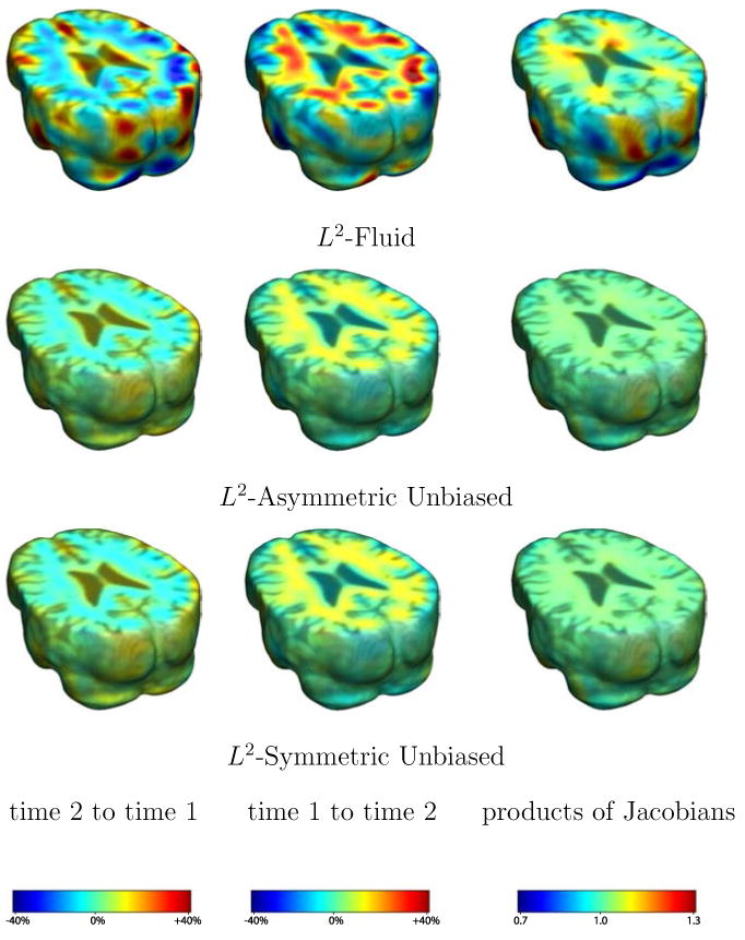
Nonrigid registration was performed on an image pair from one of the subjects from the ADNI Baseline study (serial MRI images acquired two weeks apart) using L2-Fluid (row 1), L2-Asymmetric Unbiased (row 2), and L2-Symmetric Unbiased (row 3) registration methods. Jacobian maps of deformations from time 2 to time 1 (column 1) and time 1 to time 2 (column 2) are superimposed on the target volumes. The unbiased methods generate less noisy Jacobian maps with values closer to 1; this shows the greater stability of the approach when no volumetric change is present. Column 3 examines the inverse consistency of deformation models. Products of Jacobian maps generated using all three models are shown, for forward direction (time 1 to time 2) and backward direction (time 2 to time 1). For the L2-based unbiased methods, the products of the Jacobian maps are less noisy, with values closer to 1, showing better inverse consistency.
Fig. 4.
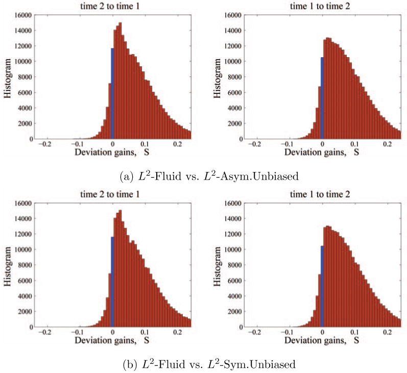
Histograms of voxel-wise deviation gains (a) L2-Fluid over L2-Asymmetric Unbiased and (b) L2-Fluid over L2-Symmetric Unbiased for one of the subjects for the forward direction (time 2 to time 1) and backward direction (time 1 to time 2). The histograms are skewed to the right, indicating the superiority of Asymmetric Unbiased and Symmetric Unbiased registration methods over Fluid registration. A paired t test shows significance (p < 0.0001). The histogram of the null distribution is centered at the point where the deviation gain S = 0, designated in blue.
Fig. 2.

Values of the L2 matching functional are shown per iteration for the L2-Fluid (solid red), L2-Asymmetric Unbiased (solid blue), and L2-Symmetric Unbiased (dashed green) methods. All methods cause the intensity mismatch measure to decrease and converge in a similar way.
Fig. 3.

(a) KL divergence and (b) SKL distance per iteration are shown for L2-Fluid (solid red), L2-Asymmetric Unbiased (solid blue), and L2-Symmetric Unbiased (dashed green) methods. For L2-Fluid, both KL and SKL measures increase, while for Asymmetric Unbiased and Symmetric Unbiased models both measures stabilize.
Of note, we have also considered a different deviation map, defined as , in place of (26). We performed statistical analyses with this definition of deviation gain, which yielded very similar results. These results are therefore not shown in this paper.
In Figure 5, we compared L2-Fluid and L2-Symmetric Unbiased methods, conducting a within-subject paired t test inside the ICBM mask for each of the ten subjects. In this case, p < 0.0001 for all subjects, indicating that the Symmetric Unbiased registration, when coupled with L2 matching cost functional, produces more reproducible maps with less variability.
Fig. 5.

Global T statistics for all ten subjects testing whether Symmetric Unbiased registration (method B) outperforms Fluid registration (method A) when coupled with L2. Here, p < 0.0001 for all subjects, indicating that the Symmetric Unbiased registration, when coupled with L2 cost functional, outperforms Fluid registration with confirmed statistical significance, producing more reproducible maps with less variability.
Group Differences
Figure 6 shows the mean Jacobian maps obtained using L2-Fluid, L2-Asymmetric Unbiased, and L2- Symmetric Unbiased registration algorithms. Jacobian maps generated using unbiased models have values closer to 1, whereas L2-Fluid model generated noisy mean maps. Figure 7, shows the results when performing 3D voxel-wise paired t tests for the deviation gain of L2-Fluid over L2-Asymmetric Unbiased and L2-Fluid over L2-Symmetric
Fig. 6.
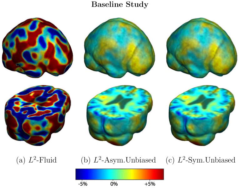
Nonrigid registration was performed on the ADNI Baseline study (serial MRI images acquired two weeks apart) of ten normal elderly subjects using L2-Fluid (column 1), L2-Asymmetric Unbiased (column 2), L2-Symmetric Unbiased (column 3) registration methods. For each method, the mean of the resulting 10 Jacobian maps is superimposed on one of the brain volumes. Visually, L2-Fluid generates a noisy mean map, while maps generated using L2-Asymmetric Unbiased and L2-Symmetric Unbiased methods are less noisy with values closer to 1. For all deformation models, regions with least stability, due to both spatial distortion and intensity inhomogeneity, are the brain stem, thalamus, and ventricles.
Fig. 7.
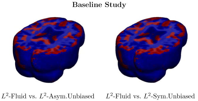
Voxel-wise paired t test for the deviation gain S empirically thresholded at 2.82 (p = 0.005 on the voxel level with 9 degrees of freedom), showing where L2-Asymmetric Unbiased and L2-Symmetric Unbiased registration outperform L2-Fluid registration (regions in red) with statistical significance on a voxel level. In contrast, there are no voxels with T values smaller than -2.82, indicating that Fluid registration does not outperform unbiased methods at any voxel. Hence, the visualization of voxel-wise paired t test with a threshold of -2.82 is omitted.
Unbiased. T maps for the deviation gains are empirically thresholded at 2.28 (p = 0.005 on the voxel level with 9 degrees of freedom) to show statistical significance.
Figure 8 shows results obtained using Multiple Comparison Analysis using permutation testing on deviation gains of L2-Fluid over L2-Symmetric Unbiased. The results indicate that out of 1024 permutations, no permutation yields a larger percentage of voxels with p < 0.05 than the observed data, which indicates that L2-Symmetric Unbiased method outperforms L2-Fluid with p < 0.001.
Fig. 8.

Multiple Comparison Analysis using permutation testing on the deviation gain S of L2-Fluid over L2-Symmetric Unbiased for baseline ADNI dataset. Each permutation randomly assigns a positive or negative sign to each of the 10 log-Jacobian maps. Here, results are plotted with respect to the number of positive signs (from 0 to 10) with 10 positive signs indicating the observed data. Dark blue, light blue, and green colors indicate the minimum, average, and maximum percentage of voxels with p < 0.05 of all possible permutations with a given number of positive signs. There is only one observation for the observed data, and thus, minimum, maximum, and average values are equal for the rightmost bar. The result indicates that out of 1024 permutations, no permutation gives a greater percentage of voxels with p < 0.05 than the observed data does. This indicates that unbiased regularization technique outperforms Fluid method with p < 0.001. Since the results obtained using Asymmetric Unbiased method are similar to those obtained using Symmetric Unbiased method, they are not shown here.
To emphasize the differences between the distributions of log Jacobian values for Fluid and unbiased (both asymmetric and symmetric) methods, in Figure 9, we plotted the cumulative distribution function of the p-values in deviation gains as defined in (27). In these plots, the interval p ∈ [0, 0.005] is the most important. For a null distribution, this cumulative plot falls along the line y = x in xy-plane, as represented by the dashed black line. Larger upward inflections of the CDF curve near the origin are associated with significant deviation gains, indicating that both Asymmetric Unbiased and Symmetric Unbiased methods outperform Fluid method in being less likely to exhibit structural changes in the absence of systematic biological changes.
Fig. 9.

Cumulative distribution of p-values for the deviation gain S of (a) L2-Fluid over L2-Asymmetric Unbiased and (b) L2-Fluid over L2-Symmetric Unbiased. Here, the ADNI baseline dataset is used. In both (a) and (b), the CDF line is well above the Null line (y = x), indicating that both asymmetric and symmetric unbiased methods outperform Fluid method (i.e. less deviation) in being less likely to exhibit structural change in the absence of biological change. Note that the interval p ∈ [0, 0.005] is of most importance for observation.
7.2 MI matching
In our second experiment, we compared the performance of methods based on mutual information matching (MI-Fluid, MI-Asymmetric Unbiased, and MI-Symmetric Unbiased). Uniform values of λ = 5 and λ = 10 were used for all deformations using MI-Symmetric Unbiased and MI-Asymmetric Unbiased algorithms, respectively. Since the Asymmetric Unbiased model quantifies only the forward deformation, the weight of the corresponding regularization functional is half the magnitude of that of the Symmetric Unbiased model, and hence, a weighting parameter twice as large should be used.
Registering Serial MRI Scans
Figures 10-13 show the results of registering a pair of serial MRI images for one of the subjects (subject 3). The deformation was computed in both directions (time 2 to time 1, and time 1 to time 2) using methods based on Mutual Information matching. In Figure 10, Jacobian maps of deformations are superimposed on brain volumes. Both Asymmetric Unbiased and Symmetric Unbiased methods generate less noisy Jacobian maps with values closer to the identity mapping, which shows the superior stability of the Unbiased approach in the absence of physiological changes. We also observed that MI-Asymmetric Unbiased and MI-Symmetric Unbiased methods to produce inverse consistent maps with less variability. Figure 11 shows the mutual information decrease per iteration for all MI-based models. Figure 12 plots the KL divergence and SKL distance measures for each of the MI-based methods. For MI-Fluid method, both KL and SKL measures increase with increasing numbers of iterations. On the other hand, these two measures stabilize for both unbiased methods. Figure 13 shows the histograms of voxel-wise deviation gains of MI-Fluid over MI-Asymmetric Unbiased as well as MI-Fluid over MI-Symmetric Unbiased. The histograms are skewed to the right, indicating the superiority of both unbiased registration methods over Fluid registration.
Fig. 10.
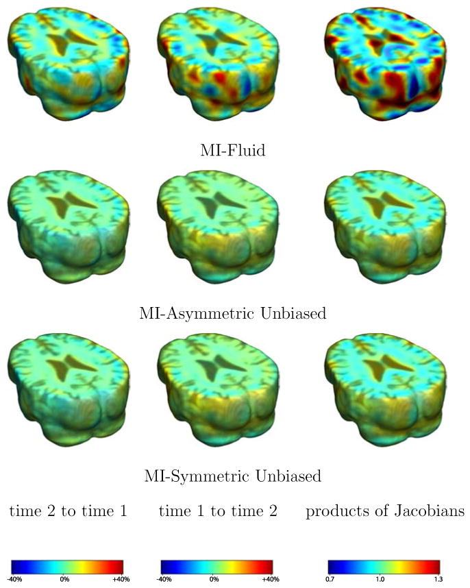
Nonrigid registration was performed on an image pair from one of the subjects from the ADNI Baseline study (serial MRI images acquired two weeks apart) using MI-Fluid (row 1), MI-Asymmetric Unbiased (row 2), and MI-Symmetric Unbiased (row 3) registration methods. Jacobian maps of deformations from time 2 to time 1 (column 1) and time 1 to time 2 (column 2) are superimposed on the target volumes. The unbiased methods generate less noisy Jacobian maps with values closer to 1; this shows the greater stability of the approach when no volumetric change is present. Column 3 examines the inverse consistency of deformation models. Products of Jacobian maps generated using all three models are shown, for the forward direction (time 1 to time 2) and backward direction (time 2 to time 1). For the mutual information-based unbiased methods, the products of the Jacobian maps are less noisy, with values closer to 1, showing better inverse consistency.
Fig. 13.
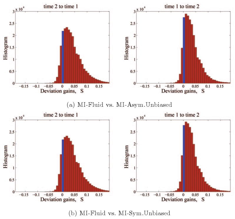
Histograms of voxel-wise deviation gains (a) MI-Fluid over MI-Asymmetric Unbiased and (b) MI-Fluid over MI-Symmetric Unbiased for one of the subjects, for the forward direction (time 2 to time 1) and backward direction (time 1 to time 2). The histograms are skewed to the right, indicating the superiority of Asymmetric Unbiased and Symmetric Unbiased registration methods over Fluid registration. Paired t test shows significance (p < 0.0001). The histogram of the null distribution is centered at the point where the deviation gain S = 0, designated in blue.
Fig. 11.

Values of the mutual information matching functional are shown per iteration for the MI-Fluid (solid red), MI-Asymmetric Unbiased (solid blue), and MI-Symmetric Unbiased (dashed green) methods. Again, all methods cause the intensity mismatch measure to decrease and converge in a similar way.
Fig. 12.

(a) KL divergence and (b) SKL distance per iteration are shown for the MI-Fluid (solid red), MI-Asymmetric Unbiased (solid blue), and MI-Symmetric Unbiased (dashed green) methods. For MI-Fluid, both KL and SKL measures increase, while for Asymmetric Unbiased and Symmetric Unbiased models both measures stabilize.
In Figure 14, we compared MI-Fluid and MI-Symmetric Unbiased methods, conducting a within-subject paired t test for each of the ten subjects. In this case, p < 0.0001 for all subjects, indicating that the Symmetric Unbiased registration, when coupled with mutual information matching cost functional, produces more reproducible maps with less variability.
Fig. 14.

Global T statistics for all ten subjects testing whether Symmetric Unbiased registration (method B) outperforms Fluid registration (method A) when coupled with mutual information. Here, p < 0.0001 for all subjects, indicating that the Symmetric Unbiased registration, when coupled with MI matching cost functional, outperforms Fluid registration with confirmed statistical significance, producing more reproducible maps with less variability.
Group Differences
Figure 15 shows the mean Jacobian maps obtained using MI-Fluid, MI-Asymmetric Unbiased, and MI- Symmetric Unbiased registration algorithms. Jacobian maps generated using unbiased models have values closer to 1, whereas MI-Fluid model generated noisy mean maps. Figure 16, shows the results when performing 3D voxel-wise paired t tests for the deviation gain of MI-Fluid over MI-Asymmetric Unbiased and MI-Fluid over MI-Symmetric Unbiased. T maps for the deviation gains are empirically thresholded at 2.28 (p = 0.005 on the voxel level with 9 degrees of freedom) to show statistical significance.
Fig. 15.
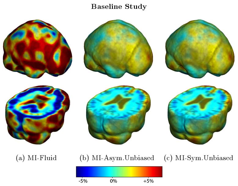
Nonrigid registration was performed on the ADNI Baseline study (serial MRI images acquired two weeks apart) of ten normal elderly subjects using MI-Fluid (column 1), and MI-Asymmetric Unbiased (column 2), and MI-Symmetric Unbiased (column 3) registration methods. For each method, the mean of the resulting 10 Jacobian maps is superimposed on one of the brain volumes. Visually, MI-Fluid generates a noisy mean map, while maps generated using MI-AU and MI-Symmetric Unbiased methods are less noisy with values closer to 1. For both deformation models, regions with least stability, due to both spatial distortion and intensity inhomogeneity, are the brain stem, thalamus, and ventricles.
Fig. 16.
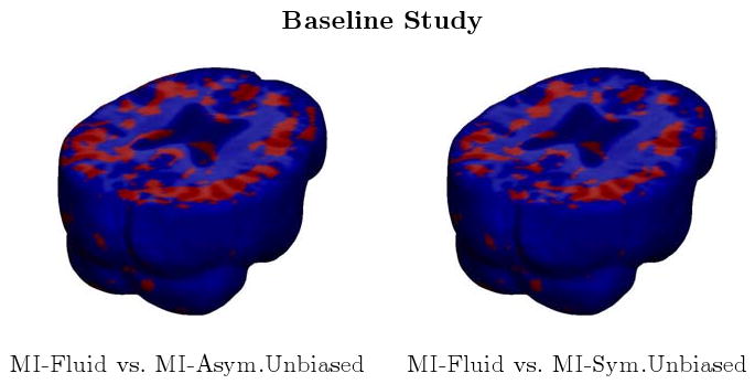
Voxel-wise paired t test for the deviation gain S empirically thresholded at 2.82 (p = 0.005 on the voxel level with 9 degrees of freedom), showing where MI-Asymmetric Unbiased and MI-Symmetric Unbiased registration outperform MI-Fluid registration (regions in red) with statistical significance on a voxel level. In contrast, there are no voxels with T values smaller than -2.82, indicating that Fluid registration does not outperform unbiased methods at any voxel. Hence, the visualization of voxel-wise paired t test with a threshold of -2.82 is omitted.
Figure 17 shows results obtained using Multiple Comparison Analysis using permutation testing on deviation gains of MI-Fluid over MI-Symmetric Unbiased. The results indicate that out of 1024 permutations, no permutation yields a larger percentage of voxels with p < 0.05 than the observed data, which indicates that MI-Symmetric Unbiased method outperforms MI-Fluid with p < 0.001.
Fig. 17.

Multiple Comparison Analysis using permutation testing on the deviation gain S of MI-Fluid over MI-Symmetric Unbiased, for baseline ADNI dataset. See caption of Figure 8 for interpretation of the results.
In Figure 18, we plotted the cumulative distribution function of the p-values in deviation gains. Larger upward inflections of the CDF curve near the origin are associated with significant deviation gains, indicating that both Asymmetric Unbiased and Symmetric Unbiased methods outperform Fluid method in being less likely to exhibit structural changes in the absence of systematic biological changes.
Fig. 18.

Cumulative distribution of p-values for the deviation gain S of (a) MI-Fluid over MI-Asymmetric Unbiased and (b) MI-Fluid over MI-Symmetric Unbiased. Here, ADNI baseline dataset is used. In both (a) and (b), the CDF line is well above the Null line, indicating that both asymmetric and symmetric unbiased methods outperform Fluid method in being less likely to exhibit structural change in the absence of biological change. Note that the interval p ∈ [0, 0.005] is of most importance for observation.
7.3 L2 versus MI matching
Lastly, we compared L2 and mutual information cost functionals for both Fluid and Symmetric Unbiased regularization. (Since Asymmetric Unbiased and Symmetric Unbiased regularizations produce similar results, we do not show the results for the asymmetric version). We again conducted within-subject paired t tests (Figure 19) as well as group paired t tests (Figure 20) on the voxel-wise deviation gains for all voxels inside the ICBM brain mask. We showed that MI-Fluid outperforms L2-Fluid with p < 0.0001. However, the result of the comparison of L2-Symmetric Unbiased and MI-Symmetric Unbiased is inconclusive.
Fig. 19.

Global T statistics for all ten subjects testing (a) whether MI-Fluid (method B) outperforms L2-Fluid (method A), and (b) whether L2-Symmetric Unbiased (method B) outperforms MI-Symmetric Unbiased (method A). MI-Fluid outperforms L2-Fluid with p < 0.0001. However, the result of the comparison of L2-Symmetric Unbiased and MI-Symmetric Unbiased is inconclusive.
Fig. 20.

Multiple Comparison Analysis using permutation testing on the deviation gain S of (a) L2-Fluid over MI-Fluid and (b) MI-Symmetric Unbiased over L2-Symmetric Unbiased, both for baseline ADNI dataset. Each permutation randomly assigns positive or negative sign to each of the 10 log-Jacobian maps. Here, results are plotted with respect to the number of positive signs (from 0 to 10) with 10 positive signs indicating the observed data. Dark blue, light blue, and green colors indicate the minimum, average, and maximum percentage of voxels with p < 0.05 of all possible permutations with a given number of positive signs. There is only one observation for the observed data, and thus, minimum, maximum, and average values are equal for the rightmost bar. The result in (a) indicates that out of 1024 permutations, no permutation gives a greater percentage of voxels with p < 0.05 than the observed data does. This indicates that MI-Fluid method outperforms L2-Fluid method with p < 0.001. However, the comparison of MI-Symmetric Unbiased and L2-Symmetric Unbiased in (b) is inconclusive. Since the results obtained using Asymmetric Unbiased method are similar to those obtained using Symmetric Unbiased method, they are not shown here.
8 ADNI Follow-up Scan Experiments
In this section, we analyze a dataset we shall call the “ADNI Follow-up” phase dataset, which includes serial MRI images (220 × 220 × 220) of ten subjects acquired one year apart. These data were collected as part of a larger study to track degenerative brain changes in MRI in 800 subjects, ages 55 to 90, including 200 elderly controls, 400 subjects with mild cognitive impairment, and 200 patients with AD. As the images are now one year apart, real anatomical changes are present, which allows methods to be compared in the presence of true biological changes.
In Figures 21 and 22, nonlinear registration was performed using Fluid, Asymmetric Unbiased, and Symmetric Unbiased methods. Visually, the Fluid method generates noisy mean Jacobian maps, while maps generated using unbiased methods suggest a volume reduction in gray matter as well as ventricular enlargement. Here, both Asymmetric Unbiased and Symmetric Unbiased methods perform equally well. Figure 23 displays the cumulative distribution of p-values for the voxel-wise log Jacobian t-maps for both ADNI Baseline and ADNI Follow-up datasets. We expect a better method to separate these two CDF curves, indicating that a real biological change has occurred between the two time points. A greater separation is accomplished when Asymmetric Unbiased and Symmetric Unbiased methods are used, while the Fluid method does not differentiate between the two datasets.
Fig. 21.
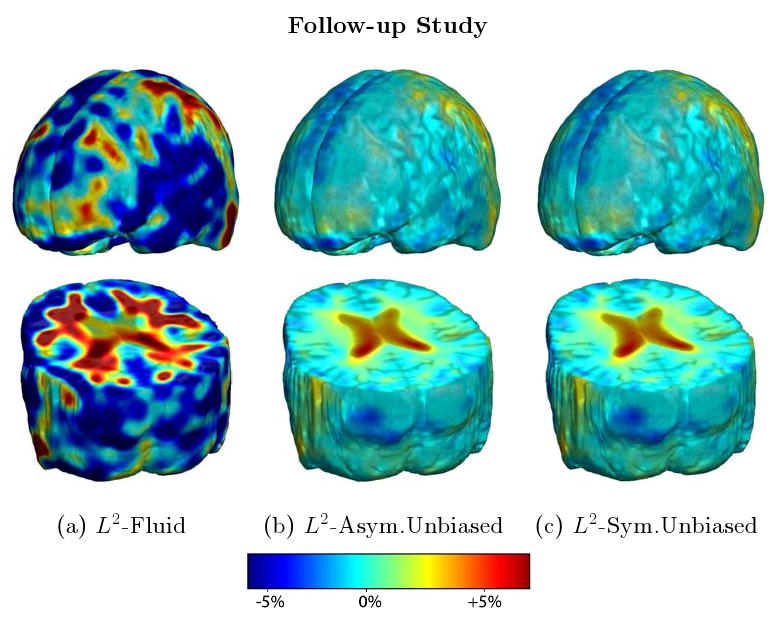
Nonrigid registration was performed on the ADNI Follow-up study (serial MRI images acquired 12 months apart) using L2-Fluid (column 1), L2-Asymmetric Unbiased (column 2), and L2-Symmetric Unbiased (column 3) registration methods. For each method, the mean of the resulting 10 Jacobian maps is superimposed on one of the brain volumes. Visually, L2-Fluid generates a noisy mean map, while maps generated using the L2-Asymmetric Unbiased and L2-Symmetric Unbiased methods suggest a volume reduction in gray matter as well as ventricular enlargement.
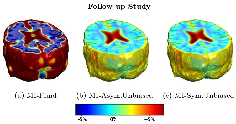
Fig. 22.
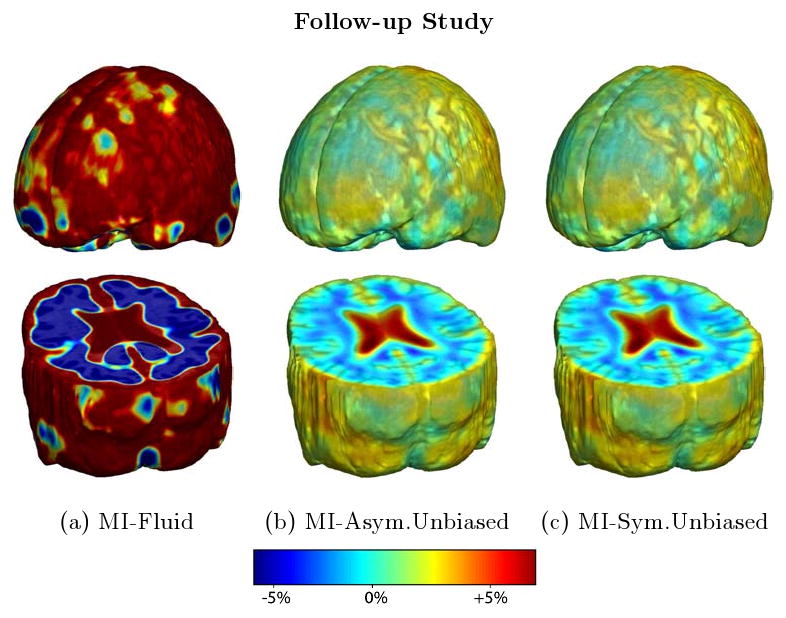
Nonrigid registration was performed on the ADNI Follow-up study (serial MRI images of patients with Alzheimer's disease acquired 12 months apart) using MI-Fluid (column 1), MI-Asymmetric Unbiased (column 2), and MI-Symmetric Unbiased (column 3) registration methods. For each method, the mean of the resulting 10 Jacobian maps is superimposed on one of the brain volumes. Visually, MI-Fluid generates a noisy mean map, while the map generated using MI-Asymmetric Unbiased and MI-Symmetric Unbiased methods suggest a volume reduction in gray matter as well as ventricular enlargement.
Fig. 23.

Cumulative distribution of p-values for the voxelwise log Jacobian t-maps (as defined in Equation (34)) for both ADNI Baseline (in blue) and Follow-up (in green) using (a) L2-Fluid, (b) L2-Asymmetric Unbiased, and (c) L2-Symmetric Unbiased methods. Here, a better method should separate these two CDF plots (see Section 5.4), indicating a real biological change has occurred between these two time points. Hence, L2-Asymmetric Unbiased and L2-Symmetric Unbiased methods outperform L2-Fluid method. Note that the interval p ∈ [0,0.005] is of most importance for observation.
In Figures 24 and 25, we further compared different registration methods by matching images artificially corrupted with Gaussian noise (zero mean; variance 12.0). Figure 25 displays the cumulative distribution of p-values for the voxel-wise log Jacobian t-maps for both ADNI Baseline and ADNI Follow-up datasets. A greater separation is accomplished when Unbiased methods are used.
Fig. 24.
Nonrigid registration was performed on the ADNI Follow-up study images artificially corrupted with Gaussian noise (mean zero; variance 12.0). For each method, the mean of the resulting 10 Jacobian maps is superimposed on one of the brain volumes.
Fig. 25.
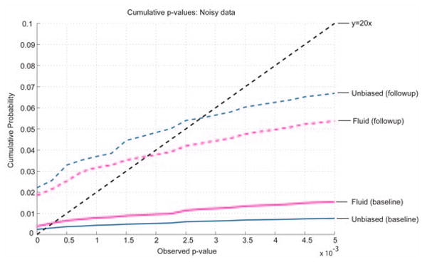
Random Gaussian noise (zero mean; variance 12.0) was added to ADNI Baseline and Follow-up datasets. Cumulative distributions of p-values for the voxelwise log Jacobian t-maps for Baseline (solid lines) and Follow-up (dashed lines) using Fluid and Unbiased methods are displayed. Here, Unbiased methods show a bigger separation between the baseline and follow-up curves, indicating that they were able to better differentiate between the two datasets.
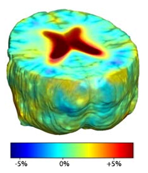
We also compared Fluid registration and Unbiased registration methods using different values for the two parameters σ and λ (Figure 26). We used λ = 1.0, 2.0, 5.0, 10.0 (for the Unbiased registration), and σ = 7,9,12 (for both Fluid and Unbiased registration). In general, Fluid registration and Unbiased registration with smaller λ values generated noisier mean maps, while maps generated using Unbiased registration with larger λ values suggest a volume reduction in gray matter as well as ventricular enlargement. As the value of the smoothing parameter σ increased, the resulting Jacobian maps became smoother, making the biological effects, such as reduction in gray matter, harder to detect.
Fig. 26.
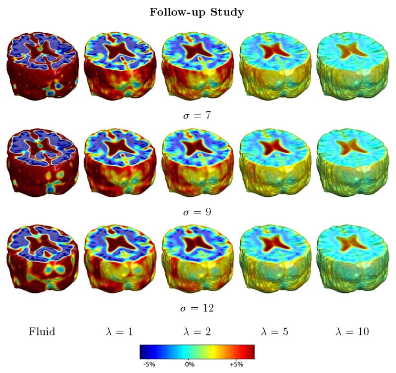
Nonrigid registration was performed on the ADNI Follow-up study using Fluid and Unbiased registration methods with different values of λ and σ. For each method, the mean of the resulting 10 Jacobian maps is superimposed on one of the brain volumes. Fluid and Unbiased registration with smaller λ values generate noisier mean maps, while maps generated using Unbiased registration with larger λ values suggest a volume reduction in gray matter as well as ventricular enlargement. As the value of the smoothing parameter σ increases, the resulting Jacobian maps become smoother, making the biological effects, such as reduction in gray matter, harder to detect.
In Figures 27 and 28, we compared Unbiased registration methods with the inverse-consistent linear elastic matching of (Christensen and Johnson (2001); Leow et al. (2005)). Figure 28 displays the cumulative distribution of p-values for the voxel-wise log Jacobian t-maps for both ADNI Baseline and Follow-up datasets for Unbiased technique with different values of λ, Fluid registration, and inverse-consistent linear elastic matching. Unbiased methods, especially with larger values of parameter λ, show a bigger separation between the baseline and follow-up curves than Fluid and inverse-consistent linear elasticity methods do, indicating that Unbiased methods, with any λ value, were able to better differentiate between the two datasets.
Fig. 27.
Inverse-consistent linear elastic registration was performed on the ADNI Follow-up study. The mean of the resulting 10 Jacobian maps is superimposed on one of the brain volumes.
Fig. 28.
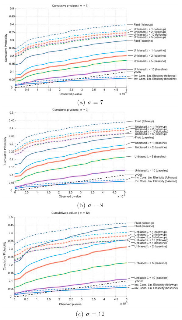
Cumulative distributions of p-values for the voxelwise log Jacobian t-maps for both ADNI Baseline (solid lines) and Follow-up (dashed lines) using Fluid, Inverse-Consistent Linear Elasticity, and Unbiased methods with different sets of parameters of λ and (a) σ = 7, (b) σ = 9, and (c) σ = 12. Unbiased methods, especially with larger values of λ, show a bigger separation between the baseline and follow-up curves than Fluid and Inverse-Consistent Linear Elasticity methods do, indicating that Unbiased methods were able to better differentiate between the two datasets.
9 Discussion
This is the first paper which aims to provide quality calibrations for different non-rigid registration techniques in TBM. We systematically investigated and compared the performances of different non-rigid registration techniques including common matching functionals (L2-metric and mutual information), and regularization techniques (fluid registration, inverse-consistent linear elastic matching, Asymmetric Unbiased, and Symmetric Unbiased techniques). Experiments were conducted to determine which registration method is more reproducible, more reliable, with less artifactual variability in regions of homogeneous image intensity. We also introduced a novel asymmetric unbiased registration model (the Asymmetric Unbiased model) and for the first time, analyzed unbiased models with mutual information based matching functionals.
We showed that both Asymmetric and Symmetric Unbiased models generate very similar results. Although in theory, the asymmetric KL regularization may potentially favor voxel expansion over the identity transformation, this is not the case globally. Indeed, given a body force of zero everywhere, the deformation with minimum asymmetric KL energy is still the identity transformation. Thus, expansion in some regions would induce contraction in others, driving overall asymmetric KL energy upwards and away from zero. Here we show that in practice, the asymmetric unbiased method does not seem to perform much differently than its symmetric version. This further supports our conclusion that the log transformation may be a more fundamental operation than symmetrization in understanding Jacobian maps in the context of medical imaging.
We compared Fluid registration and Unbiased registration methods with different values of parameters σ and λ. Fluid registration, as well as Unbiased registration with smaller values of λ, generated noisier mean maps, while maps generated using Unbiased registration with larger values of λ suggest a volume reduction in gray matter as well as ventricular enlargement. As the value of smoothing parameter σ increased, the Jacobian map became smoother, making the biological effects, such as reduction in gray matter, harder to detect.
Our analyses showed that both Asymmetric Unbiased and Symmetric Unbiased models perform significantly better than the fluid registration technique and demonstrated that the Unbiased registration, with any choice of parameters, has more power differentiating between regions of change and no change than the inverse-consistent linear elastic matching of (Christensen and Johnson (2001); Leow et al. (2005)).
The fluid registration is indeed a useful nonrigid registration technique for many applications since it generates a close alignment between the images being registered. Even so, as we showed in this paper, the fluid registration has its limitations in tensor-based morphometry. Unbiased regularization, however, ensures that the resulting deformations have intuitive axiomatic properties by penalizing any bias in the corresponding statistical maps. With Unbiased registration, we can generate accurate alignment while ensuring that deformations have intuitive axiomatic properties.
This also leads to a key issue in the field of non-linear registration, as validation studies have been relatively difficult to perform as ground truth is not generally available. Even in cases where test images were transformed using simulated deformations and thus the ground truth is known a priori, one may still wonder whether these simulated deformations correspond to anatomically plausible brain changes. As a result, efforts such as the ADNI project are important, as it provides a platform for researchers to compare nonlinear registration techniques using standardized imaging data. Along this direction, here we reported one of the first studies using the ADNI dataset, and with potentially interesting results for the rest of the registration community.
Importantly, the proposed Unbiased framework, though a novel concept in medical image registration, can be easily adapted and combined with any non-rigid registration algorithm. In this paper, we implemented the unbiased registration by adapting a fluid regularization algorithm in order to show its advantages in measuring biological deformations. The construction of Unbiased nonlinear elastic registration algorithm (Yanovsky et al. (2008a,b)) is another example of how an arbitrary nonrigid registration algorithm can be extended to compute unbiased deformations.
In addition to investigating various regularizers, we compared L2 and Mutual Information matching functionals in detecting changes in tensor-based morphometry. When applied to serial scans obtained using the same protocol, the results were inconclusive when comparing L2-Unbiased and MI-Unbiased (both asymmetric and symmetric) models. However, L2-Fluid performs less favorably than MI-Fluid. In other words, mutual information performs better as a fidelity metric when coupled with Fluid registration, but not in the case of unbiased registration.
To explain this result, we postulate that by not constraining the final deformations (as in Fluid registration), assuming intensity 1-to-1 correspondence (i.e., matching using L2) may lead to local oscillations of the deformation maps, as minimizing L2 forces a local search for the smallest intensity differences. One result of this is a Jacobian map with locally extreme values, translating into spurious signals and, in our case, less reproducibility. On the other hand, the Unbiased method eliminates local oscillations, allowing better realization of true physiological signals even when L2 is used as a data fidelity term. Again, this supports our conclusion that unbiased framework is fundamental in the understanding and realization of physiological signals.
Although various techniques have been extensively applied to detect disease effects and monitor brain changes with TBM, this paper is the first calibration study to systematically compare registration models for tensor-based morphometry. We believe our results are important, as they provide greater insight into the interpretation of TBM results in the future.
Acknowledgments
This work was supported in part by the National Institutes of Health under Grant U54 RR021813 NIH/NCRR, Grant U01 AG024904, Grant P41 RR13642, and Grant R21 EB001561. The work of Igor Yanovsky was also partially supported by NSF VIGRE Grant DMS-0601395 and CCB-NIH Grant 30886, and was also carried out in part at the Jet Propulsion Laboratory, California Institute of Technology, under a contract with the National Aeronautics and Space Administration. The work of Paul Thompson was also supported in part by the National Center for Research Resources, the National Institute for Biomedical Imaging and Bioengineering, the National Institute of Aging, and the National Institute for Neurological Disorders and Stroke, Grant R21 RR019771, Grant EB01651, Grant AG016570, Grant NS049194.
A Derivations of Gradient of R(u) in Two Spatial Dimensions
In this Appendix, we derive explicit expressions for ∂uR(u) in (18) when Ω ⊂ ℝ2. Let us denote the components of vector x to be (x1, x2) and the components of vector u be (u1, u2). We also denote ∂jui = ∂ui/∂xj.
To simplify the notation, we let J = |Dg| = |D(x – u)|. Also, denote L(J) = LKL(J) = − log J, when R = RKL and L(J) = LSKL(J) = (J – 1) log J, when R = RSKL. Note that J :  2×2(ℝ) → ℝ, where M2×2(ℝ) is the set of 2 × 2 matrices with real elements, and L : ℝ → ℝ. Jacobian J is a function of ∂jui, for i,j = 1,2, and is given by
We would like to minimize the functional
We find the first Euler-Lagrange equation. For some :
| (A.1) |
With notation L' = dL/dJ, the first Euler-Lagrange equation becomes:
| (A.2) |
Thus, minimizing the energy R(u) with respect to u1, for fixed u2, yields the first component of ∂uR(u):
| (A.3) |
Note that L'KL(J) = −1/J and L'SKL(J) = 1 + log J – 1/J.
Similarly, the Euler-Lagrange equation for the second component of ∂uR(u) can be found to be:
| (A.4) |
B Derivations of Gradient of R(u) in Three Spatial Dimensions
In this Appendix, we derive an explicit expression for ∂uR(u) in (18) when Ω ⊂ ℝ3. Let us denote the components of vector x to be (x1, x2, x3) and the components of vector u be (u1, u2, u3). Here, we will use the same notation we used in Appendix A.
Jacobian J is a function of ∂jui, for i, j = 1, 2, 3, and is given by
| (B.1) |
We would like to minimize the functional
| (B.2) |
For some η, we have
| (B.2) |
Hence, the first Euler-Lagrange equation becomes:
| (B.3) |
Thus, minimizing the energy R(u) with respect to u1, for fixed u2 and u3, yields the first component of ∂uR(u):
| (B.4) |
Similarly, the other two Euler-Lagrange equations can be found to be:
| (B.5) |
and
| (B.6) |
C Derivation of equations for maximization of Mutual Information
In this Appendix, we derive the gradient ∂uFMI(u) of the mutual information matching functional in (14), adopting the approach of (Chefd'Hotel et al. (2001); Hermosillo et al. (2001)), modeling the joint intensity distribution of deformed image I2(x − u) and image I1(x) as a continuous function using the Parzen windowing method.
We compute the first variation of FMI(u) by perturbing u in the following way
| (C.1) |
Thus, we have
| (C.2) |
However, note that
| (C.3) |
and
| (C.4) |
Hence, the second term on the right hand side of the equality in (C.2) reduces to
| (C.5) |
Equation (C.1) becomes
| (C.6) |
The joint intensity distribution estimated from I2(x − u) and I1(x) is given by
| (C.7) |
where |Ω| is a volume of Ω and ψ(ξ1,ξ2) is a two-dimensional Parzen windowing kernel.
The derivative of (C.7) can also be computed:
Let us denote
If we let ε = 0, equation (C.6) gives the first variation of FMI(u):
Here, * denotes a convolution. Thus,
| (C.8) |
Footnotes
Publisher's Disclaimer: This is a PDF file of an unedited manuscript that has been accepted for publication. As a service to our customers we are providing this early version of the manuscript. The manuscript will undergo copyediting, typesetting, and review of the resulting proof before it is published in its final citable form. Please note that during the production process errors may be discovered which could affect the content, and all legal disclaimers that apply to the journal pertain.
Contributor Information
Igor Yanovsky, Email: igor.yanovsky@jpl.nasa.gov.
Alex D. Leow, Email: feuillet@ucla.edu.
Suh Lee, Email: slee04@ucla.edu.
Stanley J. Osher, Email: sjo@math.ucla.edu.
Paul M. Thompson, Email: thompson@loni.ucla.edu.
References
- Avants B, Gee JC. Geodesic estimation for large deformation anatomical shape averaging and interpolation. NeuroImage. 2004;23 1:S139–50. doi: 10.1016/j.neuroimage.2004.07.010. [DOI] [PubMed] [Google Scholar]
- Beg M, Miller M, Trouve A, Younes L. Computing large deformation metric mappings via geodesic flows of diffeomorphisms. International Journal of Computer Vision. 2005;61(2):139–157. [Google Scholar]
- Benjamini Y, Hochberg Y. Controlling the false discovery rate: A practical and powerful approach to multiple testing. Journal of the Royal Statistical Society B. 1995;57(1):289–300. [Google Scholar]
- Broit C. PhD thesis. University of Pennsylvania; 1981. Optimal registration of deformed images. [Google Scholar]
- Brun C, Lepore N, Pennec X, Chou Y, Lopez O, Aizenstein H, Becker J, Toga A, Thompson P. Comparison of standard and Riemannian elasticity for tensor-based morphometry in HIV/AIDS. International Conference on Medical Image Computing and Computer Assisted Intervention; 2007. [DOI] [PubMed] [Google Scholar]
- Bullmore E, Suckling J, Overmeyer S, Rabe-Hesketh S, Taylor E, Brammer M. Global, voxel, and cluster tests, by theory and permutation, for a difference between two groups of structural MR images of the brain. IEEE Transactions on Medical Imaging. 1999;18:32–42. doi: 10.1109/42.750253. [DOI] [PubMed] [Google Scholar]
- Cachier P, Bardinet E, Dormont D, Pennec X, Ayache N. Iconic feature based nonrigid registration: The PASHA algorithm. Computer Vision and Image Understanding. 2003;89:272–298. [Google Scholar]
- Camara O, Schnabel J, Ridgway G, Crum W, Douiri A, Scahill R, Hill D, Fox N. Accuracy assessment of global and local atrophy measurement techniques with realistic simulated longitudinal alzheimer's disease images. NeuroImage. 2008 doi: 10.1016/j.neuroimage.2008.04.259. [DOI] [PubMed] [Google Scholar]
- Chefd'Hotel C, Hermosillo G, Faugeras O. A variational approach to multi-modal image matching. IEEE Workshop in Variational and Level Set Methods; 2001. pp. 21–28. [Google Scholar]
- Chiang M, Dutton R, Hayashi K, Lopez O, Aizenstein H, Toga A, Becker J, Thompson P. 3D pattern of brain atrophy in HIV/AIDS visualized using tensor-based morphometry. NeuroImage. 2007;34:44–60. doi: 10.1016/j.neuroimage.2006.08.030. [DOI] [PMC free article] [PubMed] [Google Scholar]
- Christensen G, Johnson H. Consistent image registration. IEEE Transactions on Medical Imaging. 2001;20(7):568–582. doi: 10.1109/42.932742. [DOI] [PubMed] [Google Scholar]
- Christensen G, Rabbitt R, Miller M. Deformable templates using large deformation kinematics. IEEE Transactions on Image Processing. 1996;5(10):1435–1447. doi: 10.1109/83.536892. [DOI] [PubMed] [Google Scholar]
- Chung M, Worsley K, Paus T, Cherif C, Collins D, Giedd J, Rapoport J, Evans A. A unified statistical approach to deformation-based morphometry. NeuroImage. 2001;14:595–606. doi: 10.1006/nimg.2001.0862. [DOI] [PubMed] [Google Scholar]
- Collignon A, Maes F, Delaere D, Vandermeulen D, Suetens P, Marchal G. Automated multi-modality image registration based on information theory. In: Bizais Y, Barillot C, Di Paola R, editors. Information Processing in Medical Imaging. Vol. 3. Kluwer Academic Publishers; Dordrecht: 1995. pp. 264–274. [Google Scholar]
- Collins D, Peters T, Evans A. Automated 3D nonlinear deformation procedure for determination of gross morphometric variability in human brain. Proceedings of the International Society for Optical Engineering (SPIE) 1994;2359:180–190. [Google Scholar]
- Crum W, Scahill R, Fox N. Automated hippocampal segmentation by regional fluid registration of serial MRI: validation and application in Alzheimer's disease. NeuroImage. 2001;13:847–855. doi: 10.1006/nimg.2001.0744. [DOI] [PubMed] [Google Scholar]
- D'Agostino E, Maes F, Vandermeulen D, Suetens P. A viscous fluid model for multimodal non-rigid image registration using mutual information. Medical Image Analysis. 2003;7:565–575. doi: 10.1016/s1361-8415(03)00039-2. [DOI] [PubMed] [Google Scholar]
- Friston K, Holmes A, Worsley K, Poline J, Frith C, Frackowiak R. Statistical parametric maps in functional imaging: A general linear approach. Human Brain Mapping. 1995;2:189–210. [Google Scholar]
- Genovese C, Lazar N, Nichols T. Thresholding of statistical maps in functional neuroimaging using the false discovery rate. Neuroimage. 2002;15:870–878. doi: 10.1006/nimg.2001.1037. [DOI] [PubMed] [Google Scholar]
- Grenander U, Miller M. Computational anatomy: An emerging discipline. Quarterly of Applied Mathematics. 1998;56:617–694. [Google Scholar]
- Gunter J, Bernstein M, Borowski B, Felmlee J, Blezek D, Mallozzi R. Validation testing of the MRI calibration phantom for the Alzheimer's Disease Neuroimaging Initiative study. International Society for Magnetic Resonance in Medicine 14th Scientific Meeting and Exhibition.2006. [Google Scholar]
- Hermosillo G, Chefd'Hotel C, Faugeras O. A variational approach to multi-modal image matching. INRIA Research report. 2001;4117 [Google Scholar]
- Hogan R, Mark L, Wang L, Joshi S, Miller M, Bucholz R. Mesial temporal sclerosis and temporal lobe epilepsy: MR imaging deformation-based segmentation of the hippocampus in five patients. Radiology. 2000;216:291–297. doi: 10.1148/radiology.216.1.r00jl41291. [DOI] [PubMed] [Google Scholar]
- Jack C, Bernstein M, Fox N, Thompson P, Alexander G, Harvey D, Borowski B, Britson P, Whitwell J, Ward C, Dale A, Felmlee J, Gunter J, Hill D, Killiany R, Schuff N, Fox-Bosetti S, Lin C, Studholme C, DeCarli C, Krueger G, Ward H, Metzger G, Scott K, Mallozzi R, Blezek D, Levy J, Debbins J, Fleisher A, Albert M, Green R, Bartzokis G, Glover G, Mugler J, Weiner M. The Alzheimer's Disease Neuroimaging Initiative (ADNI): The MR imaging protocol. Journal of Magnetic Resonance Imaging. 2008;27(4):685–691. doi: 10.1002/jmri.21049. [DOI] [PMC free article] [PubMed] [Google Scholar]
- Jovicich J, Czanner S, Greve D, Haley E, van der Kouwe A, Gollub R, Kennedy D, Schmitt F, Brown G, MacFall J, Fischl B, Dale A. Reliability in multi-site structural MRI studies: Effects of gradient non-linearity correction on phantom and human data. NeuroImage. 2006;30(2):436–443. doi: 10.1016/j.neuroimage.2005.09.046. [DOI] [PubMed] [Google Scholar]
- Klein A, Andersson J, Ardekani B, Ashburner J, Avants B, Chiang M, Christensen G, Collins D, Hellier P, Hyun P, Lepage C, Pennec X, Rueckert D, Thompson P, Vercauteren T, Woods R, Mann J, Parsey R. Evaluation of 14 nonlinear deformation algorithms applied to human brain MRI registration. NeuroImage. 2009 doi: 10.1016/j.neuroimage.2008.12.037. In press. [DOI] [PMC free article] [PubMed] [Google Scholar]
- Leow A, Huang SC, Geng A, Becker J, Davis S, Toga A, Thompson P. Inverse consistent mapping in 3D deformable image registration: Its construction and statistical properties. Information Processing in Medical Imaging. 2005;3752:493–503. doi: 10.1007/11505730_41. [DOI] [PubMed] [Google Scholar]
- Leow A, Klunder A, Jack C, Toga A, Dale A, Bernstein M, Britson P, Gunter J, Ward C, Whitwell J, Borowski B, Fleisher A, Fox N, Harvey D, Kornak J, Schuff N, Studholme C, Alexander G, Weiner M, Thompson P. Longitudinal stability of MRI for mapping brain change using tensor-based morphometry. NeuroImage. 2006;31(2):627–40. doi: 10.1016/j.neuroimage.2005.12.013. [DOI] [PMC free article] [PubMed] [Google Scholar]
- Leow A, Yanovsky I, Chiang MC, Lee A, Klunder A, Lu A, Becker J, Davis S, Toga A, Thompson P. Statistical properties of Jacobian maps and the realization of unbiased large-deformation nonlinear image registration. IEEE Transactions on Medical Imaging. 2007;26(6):822–832. doi: 10.1109/TMI.2007.892646. [DOI] [PubMed] [Google Scholar]
- Lepore N, Brun C, Pennec X, Chou Y, Lopez O, Aizenstein H, Becker J, Toga A, Thompson P. Mean template for tensor-based morphometry using deformation tensors. International Conference on Medical Image Computing and Computer Assisted Intervention; 2007. [DOI] [PubMed] [Google Scholar]
- Mazziotta J, Toga A, Evans A, Fox P, Lancaster J, Zilles K, Woods R, Paus T, Simpson G, Pike B, Holmes C, Collins D, Thompson P, MacDonald D, Schormann T, Amunts K, Palomero-Gallagher N, Parsons L, Narr K, Kabani N, Le Goualher G, Boomsma D, Cannon T, Kawashima R, Mazoyer B. A probabilistic atlas and reference system for the human brain. Journal of the Royal Society. 2001;356(1412):1293–1322. doi: 10.1098/rstb.2001.0915. [DOI] [PMC free article] [PubMed] [Google Scholar]
- Miller M. Computational anatomy: shape, growth, and atrophy comparison via diffeomorphisms. NeuroImage. 2004;23 1:S19–S33. doi: 10.1016/j.neuroimage.2004.07.021. [DOI] [PubMed] [Google Scholar]
- Morra J, Tu Z, Apostolova L, Green A, Toga A, Thompson P. Comparison of Adaboost and support vector machines for detecting Alzheimer's disease through automated hippocampal segmentation. To appear in IEEE Transactions on Medical Imaging, 2009. 2009 doi: 10.1109/TMI.2009.2021941. [DOI] [PMC free article] [PubMed] [Google Scholar]
- Nichols T, Holmes A. Nonparametric analysis of PET functional neuroimaging experiments: A primer. Human Brain Mapping. 2001;15:1–25. doi: 10.1002/hbm.1058. [DOI] [PMC free article] [PubMed] [Google Scholar]
- Nocedal J, Wright S. Numerical Optimization. Springer-Verlag; New York: 1999. [Google Scholar]
- Pieperhoff P, Sudmeyer M, Homke L, Zilles K, Schnitzler A, Amunts K. Detection of structural changes of the human brain in longitudinally acquired MR images by deformation field morphometry: Methodological analysis, validation and application. Neuroimage. 2008;43(2):269–287. doi: 10.1016/j.neuroimage.2008.07.031. [DOI] [PubMed] [Google Scholar]
- Ridha B, Barnes J, Bartlett J, Godbolt A, Pepple T, Rossor M, Fox N. Tracking atrophy progression in familial Alzheimer's disease: a serial MRI study. The Lancet Neurology. 2006;5:828–834. doi: 10.1016/S1474-4422(06)70550-6. [DOI] [PubMed] [Google Scholar]
- Shen D, Davatzikos C. Very high-resolution morphometry using mass-preserving deformations and HAMMER elastic registration. NeuroImage. 2003;18(1):28–41. doi: 10.1006/nimg.2002.1301. [DOI] [PubMed] [Google Scholar]
- Sled J, Zijdenbos A, Evans A. A nonparametric method for automatic correction of intensity nonuniformity in MRI data. IEEE Transactions on Medical Imaging. 1998;17:87–97. doi: 10.1109/42.668698. [DOI] [PubMed] [Google Scholar]
- Storey J. A direct approach to false discovery rates. Journal of the Royal Statistical Society B. 2002;64(3):479–498. [Google Scholar]
- Thompson P, Toga A. A framework for computational anatomy. Computing and Visualization in Science. 2002;5:13–34. [Google Scholar]
- Viola P, Wells W. Alignment by maximization of mutual information. International Conference on Computer Vision; 1995. pp. 16–23. [Google Scholar]
- Wang L, Swank J, Glick I, Gado M, Miller M, Morris J, Csernansky J. Changes in hippocampal volume and shape across time distinguish dementia of the Alzheimer type from healthy aging. NeuroImage. 2003;20:667–682. doi: 10.1016/S1053-8119(03)00361-6. [DOI] [PubMed] [Google Scholar]
- Wells W, Viola P, Atsumi H, Nakajima S, Kikinis R. Multi-modal volume registration by maximization of mutual information. Medical Image Analysis. 1996;1(1):35–51. doi: 10.1016/s1361-8415(01)80004-9. [DOI] [PubMed] [Google Scholar]
- Yanovsky I, Chiang MC, Thompson P, Klunder A, Becker J, Davis S, Toga A, Leow A. Quantifying deformation using information theory: The log-unbiased nonlinear registration. IEEE International Symposium on Biomedical Imaging. 2007a:13–16. [Google Scholar]
- Yanovsky I, Le Guyader C, Leow A, Thompson P, Vese L. Nonlinear elastic registration with unbiased regularization in three dimensions. The MIDAS Journal. 2008a;(549):56–67. http://hdl.handle.net/10380/1360.
- Yanovsky I, Le Guyader C, Leow A, Toga A, Thompson P, Vese L. Unbiased volumetric registration via nonlinear elastic regularization. Workshop on Mathematical Foundations of Computational Anatomy.2008b. [Google Scholar]
- Yanovsky I, Thompson P, Osher S, Leow A. Topology preserving log-unbiased nonlinear image registration: Theory and implementation. IEEE Conference on Computer Vision and Pattern Recognition; 2007b. pp. 1–8. [DOI] [PMC free article] [PubMed] [Google Scholar]
- Yeo B, Sabuncu M, Desikan R, Fischl B, Golland P. Effects of registration regularization and atlas sharpness on segmentation accuracy. Medical Image Analysis. 2008;12(5):603–615. doi: 10.1016/j.media.2008.06.005. [DOI] [PMC free article] [PubMed] [Google Scholar]
- Zhu H, Ibrahim J, Tang N, Rowe D, Xuejun H, Bansal R, Petersen B. A statistical analysis of brain morphology using wild bootstrapping. IEEE Transactions on Medical Imaging. 2007;26(7):954–966. doi: 10.1109/TMI.2007.897396. [DOI] [PMC free article] [PubMed] [Google Scholar]