Rapid Synaptic Depression Explains Nonlinear Modulation of Spectro-Temporal Tuning in Primary Auditory Cortex by Natural Stimuli

Abstract

In this study, we explored ways to account more accurately for responses of neurons in primary auditory cortex (A1) to natural sounds. The auditory cortex has evolved to extract behaviorally relevant information from complex natural sounds, but most of our understanding of its function is derived from experiments using simple synthetic stimuli. Previous neurophysiological studies have found that existing models, such as the linear spectro-temporal receptive field (STRF), fail to capture the entire functional relationship between natural stimuli and neural responses. To study this problem, we compared STRFs for A1 neurons estimated using a natural stimulus, continuous speech, with STRFs estimated using synthetic ripple noise. For about one-third of the neurons, we found significant differences between STRFs, usually in the temporal dynamics of inhibition and/or overall gain. This shift in tuning resulted primarily from differences in the coarse temporal structure of the speech and noise stimuli. Using simulations, we found that the stimulus dependence of spectro-temporal tuning can be explained by a model in which synaptic inputs to A1 neurons are susceptible to rapid nonlinear depression. This dynamic reshaping of spectro-temporal tuning suggests that synaptic depression may enable efficient encoding of natural auditory stimuli.

Introduction

Most of our understanding of sound representation in cerebral cortex comes from experiments using synthetic acoustic stimuli (Kowalski et al., 1996; deCharms et al., 1998; Blake and Merzenich, 2002; Miller et al., 2002; Gourevitch et al., 2008). Only a few studies have tested how well models of auditory processing generalize to more natural conditions in auditory cortex (Rotman et al., 2001; Machens et al., 2004) or homologous auditory systems (Theunissen et al., 2000; Nagel and Doupe, 2008). In the limited regimen of the synthetic stimuli used for model estimation, a model might accurately predict neural responses, but it is impossible to know how well that model generalizes to natural conditions unless it is tested with natural stimuli (Wu et al., 2006). The small number of experiments that have, in fact, evaluated functional models using complex natural sounds have reported that the ability of current models to generalize to novel natural stimuli is quite limited (Theunissen et al., 2000; Rotman et al., 2001; Machens et al., 2004).

In this study, we evaluated one commonly used model, the spectro-temporal receptive field (STRF), in terms of how it describes cortical responses to speech. The STRF is a linear model in the spectral domain that describes the best linear mapping between the stimulus spectrogram and the observed neural response (Aertsen and Johannesma, 1981; Kowalski et al., 1996; Klein et al., 2000; Theunissen et al., 2001; David et al., 2007). Typically, STRFs are estimated using synthetic broadband stimuli (Aertsen and Johannesma, 1981; Kowalski et al., 1996; deCharms et al., 1998; Miller et al., 2002). Broadband noise is particularly convenient because it allows for unbiased STRF estimates with computationally efficient algorithms, such as spike-triggered averaging (Klein et al., 2000). Classically, auditory neurons have been described with just a single STRF, but recent studies in the auditory cortex and avian song system have shown that STRFs depend on the stimulus used for estimation (Theunissen et al., 2000; Blake and Merzenich, 2002; Woolley et al., 2005; Gourevitch et al., 2008; Nagel and Doupe, 2008). Because auditory neurons are nonlinear, STRFs estimated from natural stimuli can vary substantially from those estimated from more commonly used synthetic stimuli (Theunissen et al., 2000; Woolley et al., 2005). These changes reflect the effects of important nonlinear mechanisms activated by natural sounds in a way that cannot be predicted from experiments with synthetic stimuli. In theory, a synthetic stimulus that contains the essential high-order statistical properties of natural sounds should activate the same response properties. However, it is not possible to produce such a synthetic stimulus until these essential statistical properties are fully characterized.

To look for stimulus-dependent STRFs in primary auditory cortex, we compared STRFs estimated using continuous speech to STRFs estimated using broadband noise composed of temporally orthogonal ripple combinations (TORCs) (Klein et al., 2000). We tested for significant differences between STRFs estimated with different stimuli by comparing their ability to predict responses in a novel data set not used for estimation (David and Gallant, 2005). To understand what spectro-temporal features of the stimuli cause the STRF changes, we also estimated STRFs from a hybrid stimulus that combined features from speech and TORCs.

Simply showing changes in STRFs estimated using different stimuli demonstrates the existence of a nonlinear response, but it does not specify the nature of the underlying mechanism (Christianson et al., 2008). To understand the mechanism that might cause different speech and TORC STRFs, we ran a series of simulations to test how different nonlinear mechanisms can give rise to stimulus-dependent STRFs. We compared three mechanisms well known in cortical neurons: short-term depression of synaptic inputs (Tsodyks et al., 1998; Wehr and Zador, 2005), divisive surround inhibition (Carandini et al., 1997), and thresholding of spiking outputs (Atencio et al., 2008). We used each of these models to simulate responses to speech and TORCs and estimated STRFs from each set of simulated responses. We then compared the tuning shifts observed for the different nonlinear models to the shifts actually observed in the neural responses. The nonlinear mechanism that more accurately predicted the observed tuning shifts was deemed the better candidate for the important mechanism for natural sound processing.

Materials and Methods

Experimental procedures

Auditory responses were recorded extracellularly from single neurons in primary auditory cortex (A1) of six awake, passively listening ferrets. All experimental procedures conformed to standards specified by the National Institutes of Health and the University of Maryland Animal Care and Use Committee.

Surgical preparation.

Animals were implanted with a steel head post to allow for stable recording. While under anesthesia (ketamine and isoflurane), the skin and muscles on the top of the head were retracted from the central 4 cm diameter of skull. Several titanium set screws were attached to the skull, a custom metal post was glued on the midline, and the entire site was covered with bone cement. After surgery, the skin around the implant was allowed to heal. Analgesics and antibiotics were administered under veterinary supervision until recovery.

After recovery from surgery, a small craniotomy (1–2 mm diameter) was opened through the cement and skull over auditory cortex. The craniotomy site was cleaned daily to prevent infection. After recordings were completed in one hemisphere, the site was closed with a thin layer of bone cement, and the same procedure was repeated in the other hemisphere.

Neurophysiology.

Single-unit activity was recorded using tungsten microelectrodes (1–5 MΩ; FHC) from head-fixed animals in a double-walled, sound-attenuating chamber (Industrial Acoustics Company). During each recording session, one to four electrodes were controlled by independent microdrives, and activity was recorded using a commercial data acquisition system (Alpha-Omega). The raw signal was digitized and bandpass filtered between 300 and 6000 Hz. Spiking events were extracted from the continuous signal using principal components analysis and k-means clustering. Only clusters with ≥90% isolation (i.e., ≥90% spikes in the cluster were likely to have been produced by a single neuron) were used for analysis. Varying the isolation threshold from 80 to 99% did not change any of the population-level effects observed in this study.

After identification of a recording site with isolatable units, a sequence of random tones (100 ms duration, 500 ms separation) was used to measure latency and spectral tuning. Neurons were verified as being in A1 according to by their tonotopic organization, latency, and simple frequency tuning (Bizley et al., 2005).

Stimuli

Stimuli were presented from digital recordings using custom software. The digital signals were transformed to analog (National Instruments), equalized to achieve flat gain (Rane), amplified to a calibrated level (Rane), and attenuated (Hewlett Packard) to the desired sound level. These signals were presented through an earphone (Etymotics) contralateral to the recording site. Before each experiment, the equalizer was calibrated according to the acoustical properties of the earphone insertion.

Stimuli from each class (described below) were presented in separate blocks, and the order of the blocks was varied randomly between experiments.

Speech.

We recorded the responses of isolated A1 neurons to segments of continuous speech. Speech stimuli, while not a complete sampling of all possible natural stimuli, are complex mammalian vocalizations that share many high-order statistical properties with a broad class of natural sounds (Smith and Lewicki, 2006). Samples of continuous speech were taken from the Texas Instruments/Massachusetts Institute of Technology (TIMIT) database (Garofolo, 1998) (see Fig. 1A). Stimuli were sentences (3–4 s) sampled each from a different speaker and balanced across gender. For each neuron, 30–90 different sentences were presented at 65 dB sound pressure level (SPL) for 5–10 repetitions. The original stimuli were recorded at 16 kHz and upsampled to 40 kHz before presentation. Included in the TIMIT database are labels of the occurrence of each phoneme, which were used to break the stimulus into its phoneme components (see Fig. 1B).

Figure 1.

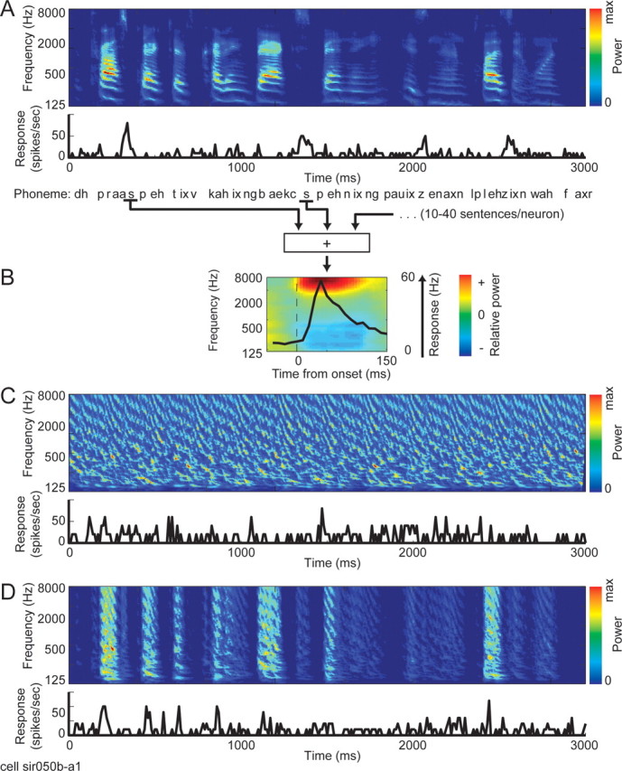
A, Spectrogram of a 3 s segment of a continuous speech stimulus. Below is the PSTH response of a single neuron to the stimulus, averaged over five repetitions. B, The strong response to high-frequency phonemes such as /s/ and /z/ in A can be visualized more clearly by computing the average response to each phoneme. The average response to /s/ for this neuron is shown overlaid on the average spectrogram of /s/. C, Spectrogram of and neuronal response to a TORC stimulus. D, Spectrogram of and neuronal response to a SPORC stimulus. The SPORC is a hybrid of the two other stimulus classes by imposing the slow temporal envelope of speech on a TORC. max, Maximum.

TORCs.

TORCs are synthetic noise stimuli designed to efficiently probe the linear spectro-temporal response properties of auditory neurons (see Fig. 1C) (Klein et al., 2000). A set of 30 TORCs probed tuning over 5 octaves (250–8000 Hz), with a spectral resolution of 1.2 cycles/octave and a temporal envelope resolution of 48 Hz (65 dB SPL, 5–10 repetitions, 3 s duration, 40 kHz sampling).

Speech-envelope orthogonal ripple combinations.

Speech-envelope orthogonal ripple combinations (SPORCs) were constructed by multiplying each of the 30 TORCs with an envelope matched to the slow modulations (∼3 Hz) associated with syllables in speech. The envelope was constructed by rectifying and low-pass filtering (300 ms Gaussian window) 30 different speech signals and multiplying each of the 30 TORCs by a different envelope. Thus, the fine spectral structure of SPORCs was nearly the same as TORCs, whereas the coarse temporal modulation structure was matched to that of speech (see Fig. 1D). As for the other stimuli, neural responses were collected for 5–10 repetitions of the SPORC set at 65 dB SPL.

STRF estimation

Linear spectro-temporal model.

Neurons in ferret A1 are tuned to stimulus frequency but are rarely phase-locked to oscillations of the sound waveform (Kowalski et al., 1996; Bizley et al., 2005). To describe tuning properties of such neurons, it is useful to represent auditory stimuli in terms of their spectrogram. The spectrogram of a sound waveform transforms the stimulus into a time-varying function of energy in each frequency band (see Fig. 1). This transformation removes the phase of the carrier signal so that the mapping from the spectrogram to neuronal firing rate can be described by a linear function.

For a stimulus spectrogram s(x,t) and instantaneous neuronal firing rate r(t) sampled at times t = 1…T, the STRF is defined as the following linear mapping (Kowalski et al., 1996; Klein et al., 2000; Theunissen et al., 2001):

Each coefficient of h indicates the gain applied to frequency channel x at time lag u. Positive values indicate components of the stimulus correlated with increased firing, and negative values indicate components correlated with decreased firing. The residual, e(t), represents components of the response (nonlinearities and noise) that cannot be predicted by the linear spectro-temporal model.

STRF estimation by boosting.

STRFs were estimated from the responses to the speech, TORC, or SPORC stimuli by boosting (Zhang and Yu, 2005; David et al., 2007). Boosting converges on an unbiased estimate of the linear mapping between stimulus and response, regardless of autocorrelation in the stimulus.

We used boosting as an alternative to normalized reverse correlation, the estimation algorithm more commonly used to estimate STRFs from natural stimuli (Theunissen et al., 2001). In a previous study, we compared these two methods and found that boosted STRFs generally were better fits and suffered less from residual correlation bias than STRFs estimated by normalized reverse correlation (David et al., 2007). Compensating for residual bias is critical for making accurate comparisons of tuning properties between STRFs estimated using different stimulus classes (David et al., 2004; Woolley et al., 2005).

Several boosting algorithms exist that can be used to estimate STRFs. In this study, we used forward stagewise fitting, which uses a simple iterative algorithm (Friedman et al., 2000). Initially, all STRF parameters are set to zero, h₀(x,y) = 0. During each iteration, i, the mean-squared error is calculated for the prediction after incrementing or decrementing each parameter by a small amount, ε. All possible increments are specified by three parameters (spectral channel, χ = 1…X; time lag, υ = 1…U; and sign, ζ = −1 or 1), such that:

Each increment can be added to the STRF from the previous iteration to provide a new predicted response:

The best increment is the one that predicts the response with the largest decrease in the mean-squared error:

This increment is added to the STRF:

and the procedure (Eqs. 2–5) is repeated until an additional increment/decrement ceases to improve model performance.

Implementing boosting requires two hyperparameters (i.e., parameters that affect the final STRF estimate but that are not determined explicitly by the stimulus/response data). These are (1) the step size, ε, and (2) the number of iterations to complete before stopping. Generally, step size can be made arbitrarily small for the best fits. However, extremely small step sizes are computationally inefficient, because they require many iterations to converge. We fixed ε to be a small fraction of the ratio between stimulus and response variance:

Here, stimulus variance is averaged across all spectral channels. Despite differences in variance across spectral channels, this heuristic produced accurate estimates and required relatively little computation time. Increasing or decreasing ε by a factor of two had no effect on STRFs. Of course, different values of ε are likely to be optimal for different data sets.

To optimize the second hyperparameter, we used an early stopping procedure. We reserved a small part (5%) of the fit data from the main boosting procedure (in addition to the reserved validation set, which was used only for final model evaluation; see below). After each iteration, we tested the ability of the STRF to predict responses in the reserved set. The optimal stopping point was reached when additional iterations ceased to improve predictions in the reserved fit data.

Thresholded STRFs.

To determine the influence of inhibitory channels on the predictive power of STRFs, we generated thresholded STRFs from the STRFs estimated using boosting. To generate thresholded STRFs, all negative coefficients in the STRF were set to zero,

Data preprocessing.

The same preprocessing was applied to all stimuli before STRF estimation. Spectrograms were generated from the stimulus sound pressure waveforms using a 128-channel rectifying filter bank that simulated processing by the auditory nerve (Yang et al., 1992). Filters had center frequencies ranging from 100 to 8000 Hz, were spaced logarithmically, and had a bandwidth of ∼1/12 octave (Q_{3 dB} = 12). To improve the signal-to-noise ratio of STRF estimates, the output of the filter bank was smoothed across frequency and downsampled to 24 channels.

Spike rates were computed by averaging responses over the 5–10 repeated stimulus presentations. Both the stimulus spectrogram and spike rates were binned at 10 ms resolution.

This data preprocessing effectively required the specification of two additional hyperparameters, the spectral and temporal sampling density. The respective values of 1/4 octave and 10 ms were chosen to match the spectral resolution of critical bands (Zwicker, 1961) and temporal resolution of neurons in A1 (Schnupp et al., 2006). Increased binning resolution would change the number of fit parameters and could, in theory, affect model performance. However, when we tested the algorithm with sparser and denser sampling of the spectral and temporal axes, we did not observe any change in the trends in tuning and predictive power across STRFs estimated with different stimuli.

Validation procedure.

A cross-validation procedure was used to make unbiased measurements of the accuracy of the different STRF models. From the entire speech data set, 95% of the data were used to estimate the STRF (estimation data set). The STRF was then used to predict the neuronal responses in the remaining 5% (validation data set), using the same 10 ms binning. This procedure was repeated 20 times, excluding a different validation segment on each repetition. Each STRF was then used to predict the responses in its corresponding validation data set. These predictions were concatenated to produce a single prediction of the neuron's response. Prediction accuracy was determined by measuring the correlation coefficient (Pearson's r) between the predicted and observed response. This procedure avoided any danger of overfitting or of bias from differences in model parameter and hyperparameter counts (David and Gallant, 2005). Each STRF was also used to predict responses to the 5% validation segments of the TORC stimulus and SPORC stimulus (when data was available), using the same procedure.

Studies using natural stimuli have argued that A1 encodes natural sounds with 10 ms resolution (Schnupp et al., 2006), but in some conditions, A1 neurons can respond with temporal resolution on the order of 4 ms (Furukawa and Middlebrooks, 2002). Measurements of prediction accuracy by correlation ignore signals at resolutions finer than the temporal window (Theunissen et al., 2001); thus, the correlation values reported in this study should not be interpreted as strict lower bounds on the portion of responses predicted by STRFs.

Tuning properties derived from STRFs

To compare STRFs estimated using the different stimulus classes, we measured seven tuning properties commonly used to describe auditory neurons (Kowalski et al., 1996; Klein et al., 2000; David et al., 2007):

Best excitatory frequency was measured by setting all negative STRF coefficients to zero and averaging along the latency axis. The resulting frequency tuning curve was smoothed with a Gaussian filter (SD, 0.2 octaves), and the best frequency was taken to be the position of the peak of the smoothed curve.

Peak excitatory latency was measured by setting all negative STRF coefficients to zero and averaging along the frequency axis. The peak latency was then taken to be the position of the peak of the resulting temporal response function.

Best inhibitory frequency and peak inhibitory latency were measured similarly to the corresponding excitatory tuning properties, but by first setting all positive, rather than negative, STRF coefficients to zero and finding the minima of the respective tuning curves after collapsing.

Spectral bandwidth describes how broad a range of frequencies excites responses from the neuron. This value was computed from the smoothed excitatory frequency tuning curve (see best excitatory frequency above) as the width, in octaves, at half-height around the best excitatory frequency.

Preferred modulation rate, measured in cycles per second or Hertz (Hz), is a complementary property to spectral bandwidth that describes the temporal modulation rate of a stimulus that best drives the neuron. Preferred rate was measured by computing the modulation transfer function of the STRF (i.e., the absolute value of its two-dimensional Fourier transform) (Klein et al., 2000; Woolley et al., 2005), averaging the first quadrant and the transpose of the second quadrant, collapsing along the spectral axis, and computing the center of mass of the average.

Gain describes the relative overall strength of a neuron's spiking response per decibel of sound energy and was computed as the SD of all coefficients in the STRF.

Simulation of nonlinear STRFs

Short-term depression model.

After stimulation, the inputs to neurons in auditory cortex are known to undergo rapid depression in their efficacy (Wehr and Zador, 2005). In neurons that undergo depression, responses decrease during rapid, repeated presentation of a stimulus but recover after extended periods of silence (on the order of tens to hundreds of milliseconds). This change in responsiveness is nonlinear and cannot be captured fully by a linear STRF. To study the effects of nonlinear depression on STRF estimates, we constructed a model neuron consisting of a bank of bandpass channels that each undergoes rapid depression (Tsodyks et al., 1998; Elhilali et al., 2004) before passing through a linear spectro-temporal filter.

In the short-term depression model, the stimulus spectrogram, s_d(x,t), was sampled over the same range of spectral channels and time bins as the original stimulus. The level of depression, d(x,t), for each channel and time bin ranged from 0 to 1. The value of d(x,t) initialized at 0 for t = 1 and was computed iteratively for subsequent time steps:

This model requires two parameters, u, the strength of depression, and τ, the time constant of recovery. A “depressed” stimulus spectrogram was then computed:

Finally, Equation 1 was used to compute the neural response but with the stimulus spectrogram replaced by s_d(x,t).

For the simulations shown in Figure 8B, u was 0.05 divided by the maximum value of s(x,t), and τ was 160 ms. Changing the values of u and τ affects the magnitude of changes in the simulated speech STRF. Larger values of u cause stronger late inhibition, and larger values of τ cause inhibition to occur at longer latencies. Reducing u and/or τ to zero cause the estimated STRF to return smoothly to the estimate for the linear STRF.

Figure 8.

A, STRFs estimated from each of the three stimulus classes for a simulated linear neuron. As expected for any neuron with linear spectro-temporal tuning, the estimated STRFs are the same as the linear filter used to generate responses. Estimates for each model are plotted using the same color scale. B, STRFs estimated using each stimulus class for a simulated neuron that undergoes rapid depression of its inputs before passing through the same linear filter as in A. The appearance of negative components at longer latencies for speech and SPORC STRFs and the reduced gain of the TORC STRF replicate the tuning differences observed for A1 neurons. C, STRFs estimated using each stimulus class for a simulated neuron that undergoes divisive normalization after passing through the same linear filter as in A. The strength of inhibition is reduced for all stimulus classes, but the temporal dynamics do not change, failing to replicate the changes observed for the A1 data. D, STRFs estimated for a simulated neuron with a high nonlinear threshold after passing through the same linear filter as in A. The absence of late inhibition in speech and SPORC STRFs and the narrowing of tuning for the speech STRF do not resemble the tuning shifts observed for the A1 data. min, Minimum; max, maximum.

Divisive normalization model.

Several studies have suggested that inhibitory lateral connections in cortex serve to provide a gain control mechanism by normalizing neural responses according to the net activity in the surrounding region on cortex (Carandini et al., 1997; Touryan et al., 2002). Although these effects have mostly been demonstrated in visual cortex, they could operate similarly in auditory cortex. To model this nonlinear mechanism, we first simulated the response of a linear neuron, r_lin(t) using Equation 1 and then normalized by the energy in the stimulus spectrogram (Carandini et al., 1997):

Unlike previous studies, this study used natural stimuli with global stimulus energy that changed rapidly over time. Thus, it was necessary to define a temporal integration window, u = U₁…U₂, for the normalization signal.

For the simulations shown in Figure 8C, we assumed that suppressive signals arrived about as quickly as excitatory inputs, with U₁ = 20 ms, and lasted as long as has been measured physiologically, U₂ = 200 ms (Wehr and Zador, 2005). (By choosing the longest duration possible, we maximized the possibility of changes in STRF dynamics, because these were the dominant stimulus-dependent effects that we observed.) In addition, two other parameters, a and b, determined the strength of normalization. For our simulations, we fixed the normalization to be strong to maximize effects on STRF estimates, with a = 0.8 divided by the average stimulus energy during U₂ − U₁ (averaged over the entire stimulus database) and b = 0.2.

Threshold model.

Another mechanism known commonly to give rise to nonlinear response properties is the spike threshold (Atencio et al., 2008; Christianson et al., 2008). Excitatory inputs must drive a neuron's membrane potential over some threshold voltage before any spikes can be elicited. We modeled threshold with positive rectification on the output of the linear filter in Equation 1. For the simulations shown in Figure 8D, the threshold was set to be very high, 2 SDs above the mean response of the linear spectro-temporal filter to the speech stimulus. Reducing the threshold to smaller values causes the estimated STRF to return to the estimate for the linear STRF.

Results

Spectro-temporal response properties of A1 neurons during stimulation by continuous speech

To study how speech is represented in primary auditory cortex (A1), we recorded the responses of 354 isolated A1 neurons to continuous speech stimuli (Fig. 1A). The stimuli were taken from a standard speech library and were sampled over an assortment of speakers, balanced between male and female (Garofolo, 1998).

To contrast the speech responses with more traditional characterizations of A1 responses, we also presented a set of TORCs to the same neurons (Fig. 1C). These stimuli are designed for efficient linear analysis of the spectro-temporal tuning properties of auditory neurons (Klein et al., 2000). Several previous studies have used TORCs or similar ripples to characterize spectro-temporal response properties in A1 (Kowalski et al., 1996; Miller et al., 2002); thus, such a characterization provides a baseline for comparing speech responses. Neuronal responses were averaged over 5–10 repeated presentations of each speech or TORC stimulus to measure a peristimulus time histogram (PSTH) for each neuron's response.

A comparison of speech and TORC spectrograms reveals basic differences in the spectro-temporal structure of the stimuli. The speech stimulus has a relatively sparse structure, in which syllables are separated by periods of silence. Neuronal responses tend to occur in brief bursts associated with the onset of syllables (Fig. 1A,B). TORCs sample spectro-temporal space uniformly, giving them a much denser spectrogram. Similarly, neural responses to TORCs tend to be much more uniformly distributed in time (Fig. 1C).

To characterize the functional relationship between the stimulus and neuronal response, we estimated the STRF for each neuron from its responses to the speech stimuli. The STRF is a linear function that maps from the stimulus spectrogram to the neuron's instantaneous firing rate response (Kowalski et al., 1996; Theunissen et al., 2001; David et al., 2007). Typically, STRFs are estimated using a standard spectrogram representation of the stimulus (Theunissen et al., 2001). To implement a more biologically plausible model, we used a spectrogram generated by a model that simulates the output of the auditory nerve with a bank of logarithmically spaced bandpass filters (Yang et al., 1992). We fit STRFs by boosting, an algorithm that minimizes the mean-squared error response predicted by the STRF while also constraining the STRF to be sparse (David et al., 2007). Several other methods exist for STRF estimation that assume different priors, such as normalized reverse correlation (Theunissen et al., 2001). The sparse prior used by boosting reduces residual stimulus bias that can complicate the comparison of STRFs estimated using different stimulus classes (Woolley et al., 2005; David et al., 2007).

We found that the STRFs estimated for A1 neurons from the speech data have bandpass spectro-temporal tuning, typical of previous measurements with TORCs (Klein et al., 2000). Figure 2A shows an example of an STRF estimated using speech. This neuron is excited by a narrow range of frequencies (best frequency, 560 Hz; peak latency, 13 ms) and shows very little inhibitory tuning.

Figure 2.

Example neuron with spectro-temporal tuning that is very similar when estimated with speech or TORCs, but with an overall gain that is higher during speech. A, The spectro-temporal receptive field (STRF) plots the tendency of a neuron to produce action potentials as a function of stimulus frequency and time lag. Areas in red indicate frequencies and time lags correlated with an increase in firing, and areas in blue indicate frequencies and lags correlated with a decrease in firing. This STRF, estimated using speech, shows an excitatory peak at 560 Hz and a peak latency of 13 ms. min, Minimum; max, maximum. B, The TORC STRF estimated for the same neuron shows very similar tuning to the speech STRF, but its overall gain is lower, indicated by the lighter shade of red in the tuning peak. (STRFs in A and B are plotted using the same color scale). C, Average spectrograms for a representative set of phonemes were computed by averaging the spectrogram of the speech stimulus over every occurrence of a phoneme. Spectrograms are each normalized to have the same maximum value. The average PSTH response of the neuron (black lines) to phonemes with energy in the 500 Hz region (/ah/and/eh/) is large, consistent with the STRF tuning. Average responses predicted by the speech STRF (blue lines) are well matched to the observed responses. Responses predicted by the TORC STRF (red lines) capture the relative response to each phoneme, but because of the weaker gain, the TORC STRF fails to predict their overall amplitude.

To test the accuracy of the STRF, we used it to predict the PSTH response to a validation speech stimulus that was also presented to the neuron but was not used for STRF estimation. The speech STRF predicts the validation stimulus quite accurately, with a correlation coefficient of r = 0.82 (10 ms time bins). The performance of the STRF can also be visualized in more detail by comparing the predicted and observed response to each phoneme, averaged across all occurrences of that phoneme in the validation set (Fig. 2C, blue and black lines, respectively). Each phoneme has a characteristic spectral signature, despite small differences across contexts (i.e., different words and speakers) (Diehl, 2008; Mesgarani et al., 2008). The PSTH predicted for each phoneme by the speech STRF is well matched to the observed neuronal response.

The STRF estimated using TORCs for the same neuron shares the same tuning properties (Fig. 2B) (best frequency, 560 Hz; latency, 13 ms). As would be expected for such a similar STRF, it predicts responses to the validation speech stimulus with nearly the same accuracy as the speech STRF (r = 0.80). However, its overall gain is lower than the speech STRF. Although this difference does not affect the prediction correlation, its effects can be seen in the average phoneme response predictions in Figure 2C. Although the TORC STRF predicts the time course and relative size of each phoneme response, it predicts a much weaker response than is actually observed (Fig. 2C, red lines). Because the correlation coefficient normalizes differences in variance, prediction correlation is not affected by global changes in gain.

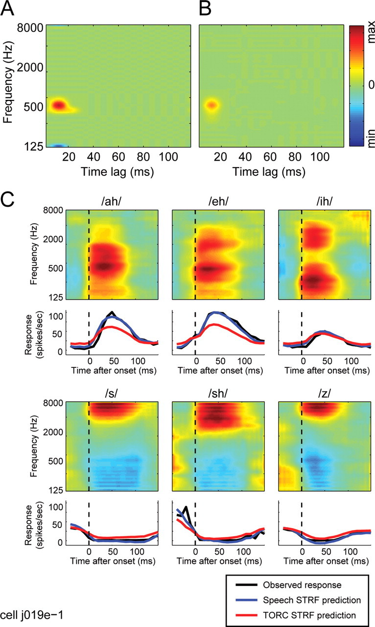
Other neurons showed a dependence of STRF shape on stimulus class. Figure 3A shows a speech STRF with excitatory tuning centered at 5200 Hz and a weak inhibitory response at later latencies. The TORC STRF estimated for the same neuron (Fig. 3B) has similar excitatory tuning but also has a large, short-latency inhibitory lobe at 7000 Hz. The speech STRF predicts responses in the validation data set (r = 0.33) significantly better than the TORC STRF, which fails completely to predict the speech responses (r = 0.01; p < 0.05, randomized paired t test).

Figure 3.

Example neuron with spectro-temporal tuning dependent on the coarse temporal structure of the stimulus used for STRF estimation. A, The speech STRF for this neuron shows excitatory tuning with a peak at 5200 Hz and 16 ms. There is also a small inhibitory lobe at 7800 Hz and 42 ms. B, The TORC STRF estimated for the same neuron shows similar excitatory tuning but has a larger inhibitory lobe at a shorter latency (peak: 7000 Hz, 19 ms). C, The SPORC STRF estimated for this neuron also has the same excitatory tuning. The inhibitory lobe is small, like the speech STRF, and falls at a latency intermediate to the speech and TORC STRFs (peak: 7000 Hz, 32 ms). D, Consistent with the tuning revealed by the STRFs, this neuron responds strongly to phonemes with energy at high frequencies (/s/,/sh/, and/z/; data plotted as in Fig. 2). Responses predicted by the speech (blue lines) and SPORC (green lines) STRFs capture the relative strength of the observed response to each phoneme. In contrast, the TORC STRF fails completely to predict these responses (red lines), attributable primarily to its large inhibitory lobe, which predicts suppression by high-frequency phonemes. min, Minimum; max, maximum.

Effects of the differences between STRFs are illustrated in the average predicted phoneme responses in Figure 3D. As in the previous example, the strength of the response to each phoneme predicted by the speech STRF is well matched to the observed response of the neuron, capturing the relatively strong responses to /s/, /sh/, and /z/. The late inhibitory component in the speech STRF may be an attempt to capture the relatively transient time course of the observed responses, although it fails to fully capture the temporal dynamics. In contrast to the speech STRF predictions, the TORC STRF predicts suppression by these three phonemes. The suppressive response can be explained by the 7000 Hz inhibitory lobe in the TORC STRF that overlaps the regions of high energy in each of the phoneme spectrograms.

One explanation for the superior performance of the speech STRF could be that spectro-temporal tuning has not changed but that the TORC STRF is simply a noisier estimate of the same function. We tested whether this is the case by comparing the ability of the STRFs to predict responses to a TORC validation stimulus. For the neuron in Figure 3, the speech STRF predicts TORC responses with a correlation of r = 0.15, whereas the TORC STRF predicts responses with a significantly greater correlation of r = 0.27 (p < 0.05, randomized paired t test). Because the TORC STRF predicts TORC responses more accurately, the differences between STRFs are not noise. Instead, they reflect a significant change in the STRF that best describes responses under the different stimulus conditions (Theunissen et al., 2001; David and Gallant, 2005).

Several different statistical features of the stimuli could be responsible for the differences between the speech and TORC STRFs in Figures 2 and 3. Speech and TORCs differ in their coarse temporal structure, which can be easily observed in the spectrograms in Figure 1, A and C, and in their fine spectro-temporal structure, observed in the correlations between spectral channels for speech (Diehl, 2008) that are absent in TORCs. To determine whether the differences between STRFs can be attributed either to coarse or fine stimulus properties, we presented a hybrid stimulus that shared structure with both speech and TORCs to a subset of 74 A1 neurons. The SPORC was generated by multiplying a TORC sound waveform with the temporal envelope of a speech stimulus. This manipulation resulted in a stimulus containing the fine temporal structure of TORCs but the coarse modulations of speech. The spectrogram of a SPORC generated from the speech and TORC examples in Figure 1 appears in Figure 1D.

The STRF estimated using SPORCs (Fig. 3C) closely resembles the speech STRF and predicts with nearly the same accuracy (r = 0.28; p > 0.2). The SPORC STRF also predicts average phoneme responses nearly as well as the speech STRF (Fig. 3D, green lines). Conversely, the SPORC STRF predicts responses in the TORC validation stimulus significantly less accurately than the TORC STRF (r = 0.20; p < 0.05). Thus, for this neuron, the differences between speech and TORC STRFs result from differences in the coarse temporal structure of the two stimuli.

Comparison of prediction accuracy between STRF classes

The tendency of speech STRFs to predict speech responses more accurately than TORC STRFs is consistent across the entire set of 354 A1 neurons in our sample. Figure 4A compares the ability of each TORC and speech STRF estimated from the same neuron to predict speech responses. The average prediction correlation for speech STRFs, r = 0.25, is significantly greater than the average for TORC STRFs, r = 0.12 (p < 0.001, randomized paired t test). It is important to note that, to avoid bias, prediction accuracy is evaluated here using a validation data set that was not used for fitting STRFs from either stimulus class (see Materials and Methods) (David and Gallant, 2005).

Figure 4.

A, Scatter plot comparing ability of speech and TORC STRFs to predict responses to speech. Across the entire sample of A1 neurons (filled and open circles), speech STRFs consistently predict better than TORC STRFs (speech STRF mean r = 0.25; TORC STRF mean r = 0.12; p < 0.001, randomized paired t test). For the 131 neurons with speech and TORC STRFs that both predict responses to their estimation stimulus with greater than random accuracy (p < 0.05, jackknifed t test; filled circles), the speech STRFs also predict significantly more accurately than the TORC STRFs (speech STRF mean r = 0.33; TORC STRF mean r = 0.21; p < 0.001, randomized paired t test). B, Scatter plot comparing ability of speech and TORC STRFs to predict responses to TORCs. In this case, TORC STRFs predict significantly better than speech STRFs both for the entire set of neurons (speech STRF mean r = 0.07; TORC STRF mean r = 0.13; p < 0.001, randomized paired t test) and for the subset that predict their own estimation stimulus class significantly (speech STRF mean r = 0.14; TORC STRF mean r = 0.23; p < 0.001, randomized paired t test). Together, these results demonstrate that STRFs estimated using the different stimulus classes are significantly different. C, When inhibitory tuning is removed by thresholding the speech and TORC STRFs, predictions by the two STRF classes are much more similar (n = 354 neurons: speech STRF mean r = 0.19, TORC STRF mean r = 0.14, p < 0.001; n = 131 significantly predicting neurons: speech STRF mean r = 0.26, TORC STRF mean r = 0.22, p < 0.001). The similarity of performance by the thresholded STRFs demonstrates that the majority of difference between STRF classes is in their inhibitory tuning.

When comparing the performance of STRFs estimated from different stimulus classes, it is also important to control for the possibility that STRFs estimated from one stimulus class may tend to be noisier than those estimated from the other. When we considered the ability of STRFs to predict responses in the validation data for their own stimulus class, we found that 282 of 354 (80%) speech STRFs predicted validation responses with greater than random accuracy (p < 0.05, jackknifed t test), whereas just 147 of 354 (42%) TORC STRFs did the same. The intersection of these two sets is a subset of 131 neurons with speech and TORC STRFs that both predict responses to their own stimulus class with greater than random accuracy (Fig. 4A, filled circles). For these neurons, the mean prediction correlation of r = 0.33 for speech STRFs is still significantly greater than the mean of r = 0.21 for TORC STRFS (p < 0.001). For 34% (44 of 131) of these neurons, the speech STRF predicts speech responses significantly better than the corresponding TORC STRF (jackknifed t test, p < 0.05). Conversely, no TORC STRF predicts speech responses significantly better than the speech STRF. This confirms that, in A1 neurons, the linear spectro-temporal tuning estimated during stimulation by speech differs systematically from tuning estimated during stimulation by TORCs.

For further confirmation that differences in STRFs do not reflect only differences in the signal-to-noise level between STRFs estimated from different stimuli, we compared the ability of speech and TORC STRFs to predict responses in the TORC validation set. In this case, TORC STRFs predict TORC responses with an average correlation of r = 0.13, which is significantly greater than the average correlation of r = 0.07 for speech STRFs (p < 0.001, randomized paired t test). The difference is also significant for the 131 neurons with STRFs that predict their own validation data with greater than random accuracy (TORC STRFs, r = 0.23; speech STRFs, r = 0.14; p < 0.001).

Predictions for all pairwise combinations of speech, TORC, and SPORC STRFs and validation data sets are summarized in Figure 5 (n = 74 neurons presented with all three stimulus classes and with STRFs that predict their own validation data with greater than random accuracy; p < 0.05, jackknifed t test). For each validation data set (i.e., validation data from each stimulus class), the best average predictor is the STRF estimated using the same stimulus class. For both speech and TORCs, the second best predictor is the SPORC STRF. In both of these cases, the SPORC STRFs predict significantly better than the third best STRFs (p < 0.001, randomized paired t test). Thus, STRFs estimated using the hybrid stimulus capture spectro-temporal properties intermediate to the two other stimulus classes.

Figure 5.

Average prediction correlations for each of the three stimulus classes (speech, TORC, and SPORC) by STRFs estimated using each stimulus class (n = 74 neurons presented with all three stimulus classes and with STRFs that predicted responses to their own validation data with greater than random accuracy; p < 0.05, jackknifed t test). For each class, the STRF estimated using that class performs significantly better than either of the others (p < 0.001, randomized paired t test). For both speech and TORC predictions, SPORC STRFs perform second best, confirming that they capture spectro-temporal tuning properties intermediate to the other stimulus conditions. The bars at the far right show average prediction correlations for speech data after thresholding the STRFs estimated from the three stimulus classes (i.e., setting all negative parameters to zero). In this case, performance by speech and SPORC STRFs are worse than the nonthresholded STRFs. The speech STRFs still perform slightly better than either other class (p < 0.01, randomized paired t test), but the overall similarity of performance suggests that the majority of difference between STRF classes is in their inhibitory tuning. NS, not significant.

Estimation stimulus primarily affects inhibitory tuning

The STRF estimated from a particular stimulus class represents a locally linear approximation of a complex nonlinear function (David et al., 2004; Nagel and Doupe, 2008). A dependence of the STRF on the estimation stimulus indicates that nonlinear response properties are activated differentially under the different stimulus conditions. To learn more about the nonlinear mechanisms that give rise to the changes in STRFs, we compared the average STRF estimate for each stimulus class. To compute the average, we aligned each STRF according to the best excitatory frequency and peak latency of that neuron (averaged across stimulus classes) and then averaged the aligned speech, TORC, and SPORC STRFs across neurons.

The average STRF for each stimulus class appears in Figure 6 (left column). For all three classes, excitatory tuning is quite similar. Inhibitory tuning varies substantially with respect to excitatory tuning, rendering the average inhibitory tuning much weaker than excitatory tuning in the average STRFs. However, if excitatory components are removed, then the average inhibitory tuning can be visualized more clearly (Fig. 6, right column). Inspection of the inhibitory tuning shows clear differences between stimulus classes. For speech STRFs (Fig. 6A), inhibitory tuning occurs over a wide range of frequencies and latencies. For TORC STRFs (Fig. 6B), inhibitory tuning is concentrated in frequency bands adjacent to excitatory tuning and mostly at short latencies similar to the latency of excitatory tuning. For SPORC STRFs (Fig. 6C), inhibitory tuning is broader and ranges over longer latencies, like speech STRFs. Thus, the tuning of inhibition differs dramatically between speech and TORC STRFs, whereas inhibition in the SPORC STRFs shows a greater resemblance to that of the speech STRFs.

Figure 6.

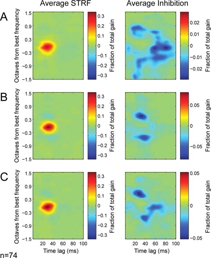
A, Average STRF (n = 74 neurons) estimated using speech, aligned to have the same best frequency and peak latency (each best frequency and latency was fixed for a single neuron across stimulus conditions). The right panel shows the average of only the negative (i.e., relative inhibitory) parameters of the STRFs. B, Average STRF estimated using TORCs. The average STRF has slightly narrower excitatory tuning than the speech STRF. Greater differences can be observed in the average inhibitory components (right), which tend to occur at shorter latencies than in speech STRFs. C, The average STRF estimated using SPORCs is similar to that for speech, although inhibition maintains some resemblance to the average TORC STRF.

To perform a quantitative comparison of tuning between stimulus classes, we measured seven tuning properties for each STRF: best excitatory frequency, best inhibitory frequency, peak excitatory latency, peak inhibitory latency, spectral bandwidth, preferred modulation rate (i.e., inverse of temporal bandwidth), and total gain. Figure 7 compares the mean value of each tuning property measured from speech, TORC, and SPORC STRFs for the 74 neurons tested with all three stimulus classes. As suggested by the average STRFs in Figure 6, average peak excitatory and inhibitory frequency are not significantly different between classes (p > 0.05, randomized paired t test), nor is the peak latency of excitation (p > 0.05). However, other tuning properties do show differences. Average peak inhibitory latency is longer (p < 0.001), and bandwidth and preferred rate are both greater for speech and SPORC STRFs than for TORC STRFs (p < 0.001). Overall gain is also significantly greater for speech and SPORC STRFs (p < 0.001).

Figure 7.

Comparison of mean tuning properties measured from speech, TORC, and SPORC STRFs. Bars for each tuning properties are normalized to have a mean of one, and the actual average value is printed above each bar. Basic tuning properties [best frequency (BF), peak excitatory latency] do not differ significantly between stimulus classes. However, the latency of inhibition is longer, the preferred modulation rate is higher, and the overall gain is higher for both speech and SPORC STRFs than for TORC STRFs (p < 0.001, randomized paired t test). These shifts in inhibitory tuning are consistent with the observation that inhibitory tuning explains differences in predictive power between STRF classes. NS, Not significant.

In contrast to the large differences between speech and TORC STRFs, there are no significant differences in average tuning between speech and SPORC STRFs. The similarity of these STRFs suggests that the major differences between speech and TORC STRFs result from differences in the coarse temporal properties of the estimation stimuli.

Changes in inhibitory tuning influence prediction accuracy

The comparison of tuning between stimulus classes reveals that inhibitory tuning is particularly dependent on the stimulus class used for estimation. Thus, the pattern of inhibition observed in speech STRFs could explain their superior ability over TORC STRFs to predict responses to speech. To measure the contribution of inhibitory tuning to prediction accuracy directly, we applied a threshold to each STRF, setting all negative coefficients to zero and effectively removing inhibitory tuning (Eq. 7). We compared the ability of these thresholded STRFs to predict responses to speech (Fig. 4C). After thresholding, prediction accuracy of speech STRFs decreased (mean r = 0.26; n = 131; p < 0.001, randomized paired t test), whereas the prediction accuracy of TORC STRFs did not change significantly (mean r = 0.22; p > 0.05, randomized paired t test). For each neuron, the performance of the two STRFs tended to be much more similar than for STRFs before thresholding, as can be seen in the relatively tight clustering near the line of unity slope in Figure 4C.

When the same thresholding procedure was applied to SPORC STRFs, the mean prediction correlation for speech was significantly reduced to r = 0.21 (Fig. 5) (n = 74; p < 0.01, randomized paired t test). This decrease indicates that, unlike TORC STRFs, the inhibitory tuning expressed in SPORC STRFs contributes to prediction accuracy and is actually characteristic of activity during processing of speech. Removing inhibitory components drives all three STRF classes to perform similarly, suggesting that the majority of their differences lie in their inhibitory tuning. However, the thresholded speech STRFs do still predict speech responses slightly better than the TORC and SPORC STRFs (p < 0.01, randomized paired t test). The small remaining differences in prediction accuracy are presumably attributable to changes in excitatory tuning specific to the fine spectro-temporal structure of speech (Blake and Merzenich, 2002; Gourevitch et al., 2008).

Rapid synaptic depression can explain differences between speech and TORC STRFs

The differences between STRFs estimated using speech and TORCs suggests that a nonlinear mechanism is differentially activated under the different stimulus conditions (David et al., 2004; Woolley et al., 2005; Nagel and Doupe, 2008). However, the existence of a difference between STRFs does not in itself indicate what particular nonlinear mechanisms are important for creating the difference. A wide range of nonlinear response properties are known to exist in cortex, including rapid synaptic depression (Wehr and Zador, 2005), divisive normalization (Carandini et al., 1997), and thresholding (Atencio et al., 2008). We wanted to determine whether the pattern of changes observed between STRFs could provide insight into the nonlinearity responsible for the changes. To answer this question, we simulated the responses of auditory neurons with different nonlinear mechanisms. We compared four models: (1) a simple linear spectro-temporal filter; (2) a spectro-temporal filter with inputs that undergo rapid nonlinear synaptic depression (Tsodyks et al., 1998; Elhilali et al., 2004); (3) a spectro-temporal filter with output that undergoes divisive normalization (Carandini et al., 1997); and (4) a spectro-temporal filter with output that passes through a nonlinear threshold (Atencio et al., 2008). For each model, we simulated the responses of a neuron with the same underlying spectro-temporal filter to the three stimulus classes used in this study. We then estimated STRFs for the different simulation/stimulus class combinations using the same methodology as for the actual A1 data.

Figure 8A shows STRFs estimated for the simple linear filter. As would be expected (Theunissen et al., 2001), the STRFs are the same for all three stimulus classes. The pattern of spectro-temporal tuning in the estimates (excitatory lobe at 2000 Hz and weaker inhibitory lobe at 800 Hz) matches the original linear filter used to generate the simulated responses.

Unlike the linear model, STRFs estimated for the simulation with rapidly depressing inputs vary substantially between stimulus classes (Fig. 8B). All three STRFs have inhibition at latencies following the excitatory lobe. However, the latency is longer for the speech and SPORC STRFs than for the TORC STRF. Gain also differs substantially between STRFs. The overall excitatory gain of the SPORC STRF is nearly the same as the speech STRF, whereas the gain of the TORC STRF is substantially lower. The exact magnitude of changes between stimulus classes depends on the strength of depression and recovery time constant specified in the model (Eq. 8). However, it is clear that the differences between stimulus classes resemble the pattern observed in the A1 data (Figs. 6, 7).

Estimated STRFs for the divisive normalization simulation (Fig. 8C) also vary between stimulus classes, but they follow a much different pattern. The strength of inhibition is reduced, most prominently for the speech STRF, but the tuning of inhibition does not change with the stimulus. This pattern does not match the changes observed in the A1 data, because there is no difference in the time course of inhibition, and the SPORC STRF more closely resembles the TORC STRF than the speech STRF.

Estimated STRFs for the output threshold simulation (Fig. 8D) also follow a different pattern than the observed data. In this case, the speech STRF is more narrowly tuned along the spectral axis, and inhibition is reduced. Both the TORC and SPORC STRFs show tuning very similar to the linear model. Thus, the threshold model also does not predict similar shifts in tuning for the speech and SPORC STRFs

These simulations suggest that rapid depression of inputs to A1 neurons can give rise to the pattern of changes observed between STRFs estimated using speech and TORCs. Speech contains relatively long periods of silence between phonemes that give it a sparse temporal structure compared with TORCs (Fig. 1, compare spectrograms in A, C). During the silence between phonemes, depressed inputs have the opportunity to recover so that they can produce strong transient responses to the onset of the next phoneme. When the same simulation was run with SPORC stimuli, it predicted that SPORC STRFs should share spectro-temporal tuning properties with speech STRFs, which is also confirmed in our data (Figs. 6, 7). The slightly longer inhibition in the speech STRF than the SPORC STRF results from the 300 ms smoothing that was applied to the SPORC envelope (see Materials and Methods). This smoothing diminished the sharp onsets and offsets in the speech stimulus, reducing the amount of time for recovery from depression. This slight difference is also reflected in the actual A1 data in Figure 6, where the inhibitory tuning in the average SPORC STRF shows less late inhibitory tuning than the average speech STRF.

Discussion

We have shown that STRFs estimated for neurons in primary auditory cortex (A1) show a strong dependence on the class of stimuli used for estimation. Specifically, the latency and spectral tuning of inhibition varies systematically between STRFs estimated using continuous speech and TORCs. During stimulation by speech, A1 neurons tend to have a longer latency of inhibition and a higher overall gain than during stimulation by TORCs. These systematic tuning differences explain much of the ability of speech STRFs to predict neuronal responses to speech better than TORC STRFs.

Stimulus dependence of spectro-temporal tuning can be explained by rapid synaptic depression

A dependency of STRFs on the stimulus class used for estimation indicates that a nonlinear response mechanism is being activated differentially, according to the spectro-temporal properties of the estimation stimulus (Theunissen et al., 2001; David et al., 2004; Nagel and Doupe, 2008). Stimulus-dependent STRFs have been reported previously for synthetic stimuli in auditory cortex (Blake and Merzenich, 2002; Gourevitch et al., 2008). In addition, stimulus-dependent STRFs have been reported for natural stimuli in areas analogous to auditory cortex in the songbird (Theunissen et al., 2000; Nagel and Doupe, 2008) and in visual cortex (David et al., 2004). However, little is known about the specific nonlinear mechanisms that underlie such changes in any system.

In this study, we compared speech and TORC STRFs for a large number of neurons to identify systematic changes between them. The changes that we observed in inhibitory tuning were consistent with a nonlinear model in which inputs to A1 neurons undergo rapid depression after stimulation (Tsodyks et al., 1998). Such depression is biologically plausible and has previously been proposed as a mechanism for controlling the precise timing of spikes in response to modulated stimuli in A1 (Elhilali et al., 2004). Theoretical studies have also suggested that rapid synaptic depression controls temporal dynamics and gain control in the visual system (Chance et al., 1998).

The rapid depression model predicts that a hybrid stimulus that combines the coarse temporal modulations of speech with the fine structure of TORCs should produce STRFs similar to speech STRFs. When we measured STRFs with such a hybrid stimulus, we found, in fact, that the resulting STRFs have tuning properties similar to speech STRFs. Alternative nonlinear models that incorporated surround normalization or a high spiking threshold into the neural response did not predict the same shift in inhibitory tuning, nor did they predict that STRFs estimated from the hybrid stimulus should resemble speech STRFs. Some differences did persist between STRFs estimated using speech and the hybrid stimulus. These differences reflect the effects of the fine spectro-temporal structure of speech, perhaps local changes in spectral density or bandwidth, which have been shown to modulate STRFs in A1 (Blake and Merzenich, 2002; Gourevitch et al., 2008).

Our findings agree with other studies that suggest that different mechanisms may contribute to inhibitory tuning in A1 (Sutter and Loftus, 2003). Inhibitory tuning (i.e., a decrease in responses correlated with an increase in stimulus power) at longer latencies may result from synaptic depression, whereas inhibition at shorter latencies may arise by a different mechanism, such as direct inhibitory inputs from neighboring cortical neurons (Wehr and Zador, 2005).

Our findings suggest that rapid depression is a dominant nonlinear mechanism in primary auditory cortex that can explain much of the stimulus dependence of STRFs. Additional experiments can confirm this hypothesis by measuring STRFs with different stimulus classes and comparing those results with predictions by the rapid depression model. These findings also predict that a nonlinear model that accounts explicitly for synaptic depression should provide a better description of responses in A1. A similar nonlinear model has shown improved ability over the linear STRF to predict responses to random chord stimuli (Ahrens et al., 2008). In theory, incorporating the appropriate synaptic depression mechanism into the input stage of the linear STRF may accomplish this goal (Gill et al., 2006). However, because synaptic depression effects vary across neurons, depression parameters must be fit individually for each neuron to significantly improve model performance. Fitting such a model would require a nonlinear regression algorithm outside the scope of the boosting procedure used in this study, such as an iterative procedure that alternately updates STRF coefficients and other nonlinear terms (Ahrens et al., 2008).

Depression enables dynamic shifts in spectro-temporal tuning for processing natural sounds

According to our simulations, rapid synaptic depression can give rise to apparently inhibitory regions in the STRF that match the best frequency of the neuron but appear at time lags after an initial excitatory peak. Such dynamics allow a neuron to give an initial strong transient response to a stimulus after a period of silence, which is then rapidly attenuated during a sustained stimulus. During stimulation by speech, the depression mechanism can recover over the relatively long silent periods between syllables. However, during stimulation by TORCs, stimuli are presented nearly constantly, preventing the depression from ever recovering. Because of the dynamic changes in the state of synaptic depression, the spectro-temporal information represented during speech stimulation can change over the course of stimulus presentation. This mechanism may allow cortex to efficiently extract useful information from auditory stimuli as it becomes available.

Many animal vocalizations share the impulsive (i.e., temporally sparse burst) structure of speech, because they are composed of a sequence of complex spectro-temporal syllables, separated by periods of silence (Smith and Lewicki, 2006). Thus, spectro-temporal response properties observed during speech stimulation are likely to resemble the responses that occur during the processing of other natural sounds. In the bird song system, Field L neurons that show delayed inhibition are particularly important for discriminating between different song stimuli (Narayan et al., 2005). Delayed inhibition is exactly the feature that appears in STRFs during speech stimulation, which we attribute to synaptic depression. Thus, dynamic changes in the state of synaptic depression may contribute to the improved discriminative power of these Field L neurons.

It has been proposed that changes in STRFs reflect adaptation to the spectro-temporal statistics of a particular natural stimulus for optimal representation of that stimulus (Woolley et al., 2005). Although the changes we observe in STRFs are consistent with such adaptation, these changes do not necessarily represent a generic ability to adapt to any stimulus. Instead, our findings suggest that rapid synaptic depression enables efficient processing specifically of vocalizations and similar natural sounds. This finding does not necessitate that STRFs will adapt to the spectro-temporal statistics of an arbitrarily constructed synthetic stimulus that does not share properties with natural stimuli.

Linear STRFs provide a tool for characterizing nonlinear response properties

As a tool for understanding auditory representation, STRFs have sometimes been criticized for being unable to characterize critical nonlinearities involved in the processing of sounds (Atencio et al., 2008; Christianson et al., 2008). Whereas these concerns warrant special attention when studying STRFs, they do not necessarily invalidate the methodology. As we demonstrate in this study, the effects of nonlinear responses can give rise to systematic differences between STRFs. By identifying these systematic differences, it is possible to infer properties of the nonlinear mechanisms that cause them and compare how well different nonlinear models predict the observed effects. By following such logic in this study, we were able to compare the likely influence of rapid synaptic depression, divisive normalization, and output thresholding.

By estimating STRFs under a large number of stimulus conditions, it may be possible to fully reconstruct the underlying nonlinear model (David et al., 2004; Wu et al., 2006; Nagel and Doupe, 2008). Of course, the amount of data available for analysis is critically limited by the constraints of neurophysiology experiments. Such an effort can be performed more effectively by a combination of simulation and experimentation. As in this study, a simulation can predict that a particular nonlinear mechanism should give rise to differences between STRFs estimated using two different stimuli, whereas a different nonlinearity will not. Experiments comparing STRFs between these stimulus conditions can then test which nonlinear mechanism actually influences neural responses. This general approach of comparing model fits under different stimulus conditions is not restricted to the study of STRFs and can be applied to other model frameworks as well (Touryan et al., 2005; Atencio et al., 2008).

References

- Aertsen AM, Johannesma PI. The spectro-temporal receptive field. A functional characteristic of auditory neurons. Biol Cybern. 1981;42:133–143. doi: 10.1007/BF00336731. [DOI] [PubMed] [Google Scholar]
- Ahrens MB, Linden JF, Sahani M. Nonlinearities and contextual influences in auditory cortical responses modeled with multilinear spectrotemporal methods. J Neurosci. 2008;28:1929–1942. doi: 10.1523/JNEUROSCI.3377-07.2008. [DOI] [PMC free article] [PubMed] [Google Scholar]
- Atencio CA, Sharpee TO, Schreiner CE. Cooperative nonlinearities in auditory cortical neurons. Neuron. 2008;58:956–966. doi: 10.1016/j.neuron.2008.04.026. [DOI] [PMC free article] [PubMed] [Google Scholar]
- Bizley JK, Nodal FR, Nelken I, King AJ. Functional organization of ferret auditory cortex. Cereb Cortex. 2005;15:1637–1653. doi: 10.1093/cercor/bhi042. [DOI] [PubMed] [Google Scholar]
- Blake DT, Merzenich MM. Changes of AI receptive fields with sound density. J Neurophysiol. 2002;88:3409–3420. doi: 10.1152/jn.00233.2002. [DOI] [PubMed] [Google Scholar]
- Carandini M, Heeger DJ, Movshon JA. Linearity and normalization in simple cells of the macaque primary visual cortex. J Neurosci. 1997;17:8621–8644. doi: 10.1523/JNEUROSCI.17-21-08621.1997. [DOI] [PMC free article] [PubMed] [Google Scholar]
- Chance FS, Nelson SB, Abbott LF. Synaptic depression and the temporal response characteristics of V1 cells. J Neurosci. 1998;18:4785–4799. doi: 10.1523/JNEUROSCI.18-12-04785.1998. [DOI] [PMC free article] [PubMed] [Google Scholar]
- Christianson GB, Sahani M, Linden JF. The consequences of response nonlinearities for interpretation of spectrotemporal receptive fields. J Neurosci. 2008;28:446–455. doi: 10.1523/JNEUROSCI.1775-07.2007. [DOI] [PMC free article] [PubMed] [Google Scholar]
- David SV, Gallant JL. Predicting neuronal responses during natural vision. Network. 2005;16:239–260. doi: 10.1080/09548980500464030. [DOI] [PubMed] [Google Scholar]
- David SV, Vinje WE, Gallant JL. Natural stimulus statistics alter the receptive field structure of V1 neurons. J Neurosci. 2004;24:6991–7006. doi: 10.1523/JNEUROSCI.1422-04.2004. [DOI] [PMC free article] [PubMed] [Google Scholar]
- David SV, Mesgarani N, Shamma SA. Estimating sparse spectro-temporal receptive fields with natural stimuli. Network. 2007;18:191–212. doi: 10.1080/09548980701609235. [DOI] [PubMed] [Google Scholar]
- deCharms RC, Blake DT, Merzenich MM. Optimizing sound features for cortical neurons. Science. 1998;280:1439–1443. doi: 10.1126/science.280.5368.1439. [DOI] [PubMed] [Google Scholar]
- Diehl RL. Acoustic and auditory phonetics: the adaptive design of speech sound systems. Philos Trans R Soc Lond B Biol Sci. 2008;363:965–978. doi: 10.1098/rstb.2007.2153. [DOI] [PMC free article] [PubMed] [Google Scholar]
- Elhilali M, Fritz JB, Klein DJ, Simon JZ, Shamma SA. Dynamics of precise spike timing in primary auditory cortex. J Neurosci. 2004;24:1159–1172. doi: 10.1523/JNEUROSCI.3825-03.2004. [DOI] [PMC free article] [PubMed] [Google Scholar]
- Friedman J, Hastie T, Tibshirani R. Additive logistic regression: a statistical view of boosting. Ann Stat. 2000;28:337–407. [Google Scholar]
- Furukawa S, Middlebrooks JC. Cortical representation of auditory space: information-bearing features of spike patterns. J Neurophysiol. 2002;87:1749–1762. doi: 10.1152/jn.00491.2001. [DOI] [PubMed] [Google Scholar]
- Garofolo J. Getting started with the DARPA TIMIT CD-ROM: an acoustic phonetic continuous speech database. Gaithersburg, MD: National Institute of Standards and Technology; 1998. [Google Scholar]
- Gill P, Zhang J, Woolley SM, Fremouw T, Theunissen FE. Sound representation methods for spectro-temporal receptive field estimation. J Comput Neurosci. 2006;21:5–20. doi: 10.1007/s10827-006-7059-4. [DOI] [PubMed] [Google Scholar]
- Gourevitch B, Norena A, Shaw G, Eggermont JJ. Spectrotemporal receptive fields in anesthetized cat primary auditory cortex are context dependent. Cereb Cortex. 2008 doi: 10.1093/cercor/bhn184. [DOI] [PubMed] [Google Scholar]
- Klein DJ, Depireux DA, Simon JZ, Shamma SA. Robust spectrotemporal reverse correlation for the auditory system: optimizing stimulus design. J Comput Neurosci. 2000;9:85–111. doi: 10.1023/a:1008990412183. [DOI] [PubMed] [Google Scholar]
- Kowalski N, Depireux DA, Shamma SA. Analysis of dynamic spectra in ferret primary auditory cortex. I. Characteristics of single-unit responses to moving ripple spectra. J Neurophysiol. 1996;76:3503–3523. doi: 10.1152/jn.1996.76.5.3503. [DOI] [PubMed] [Google Scholar]
- Machens CK, Wehr MS, Zador AM. Linearity of cortical receptive fields measured with natural sounds. J Neurosci. 2004;24:1089–1100. doi: 10.1523/JNEUROSCI.4445-03.2004. [DOI] [PMC free article] [PubMed] [Google Scholar]
- Mesgarani N, David SV, Fritz JB, Shamma SA. Phoneme representation and classification in primary auditory cortex. J Acoust Soc Am. 2008;123:899–909. doi: 10.1121/1.2816572. [DOI] [PubMed] [Google Scholar]
- Miller LM, Escabi MA, Read HL, Schreiner CE. Spectrotemporal receptive fields in the lemniscal auditory thalamus and cortex. J Neurophysiol. 2002;87:516–527. doi: 10.1152/jn.00395.2001. [DOI] [PubMed] [Google Scholar]
- Nagel KI, Doupe AJ. Organizing principles of spectro-temporal encoding in the avian primary auditory area field L. Neuron. 2008;58:938–955. doi: 10.1016/j.neuron.2008.04.028. [DOI] [PMC free article] [PubMed] [Google Scholar]
- Narayan R, Ergun A, Sen K. Delayed inhibition in cortical receptive fields and the discrimination of complex stimuli. J Neurophysiol. 2005;94:2970–2975. doi: 10.1152/jn.00144.2005. [DOI] [PubMed] [Google Scholar]
- Rotman Y, Bar-Yosef O, Nelken I. Relating cluster and population responses to natural sounds and tonal stimuli in cat primary auditory cortex. Hear Res. 2001;152:110–127. doi: 10.1016/s0378-5955(00)00243-4. [DOI] [PubMed] [Google Scholar]
- Schnupp JW, Hall TM, Kokelaar RF, Ahmed B. Plasticity of temporal pattern codes for vocalization stimuli in primary auditory cortex. J Neurosci. 2006;26:4785–4795. doi: 10.1523/JNEUROSCI.4330-05.2006. [DOI] [PMC free article] [PubMed] [Google Scholar]
- Smith EC, Lewicki MS. Efficient auditory coding. Nature. 2006;439:978–982. doi: 10.1038/nature04485. [DOI] [PubMed] [Google Scholar]
- Sutter ML, Loftus WC. Excitatory and inhibitory intensity tuning in auditory cortex: evidence for multiple inhibitory mechanisms. J Neurophysiol. 2003;90:2629–2647. doi: 10.1152/jn.00722.2002. [DOI] [PubMed] [Google Scholar]
- Theunissen FE, Sen K, Doupe AJ. Spectral-temporal receptive fields of non-linear auditory neurons obtained using natural sounds. J Neurosci. 2000;20:2315–2331. doi: 10.1523/JNEUROSCI.20-06-02315.2000. [DOI] [PMC free article] [PubMed] [Google Scholar]
- Theunissen FE, David SV, Singh NC, Hsu A, Vinje WE, Gallant JL. Estimating spatial temporal receptive fields of auditory and visual neurons from their responses to natural stimuli. Network. 2001;12:289–316. [PubMed] [Google Scholar]
- Touryan J, Lau B, Dan Y. Isolation of relevant visual features from random stimuli for cortical complex cells. J Neurosci. 2002;22:10811–10818. doi: 10.1523/JNEUROSCI.22-24-10811.2002. [DOI] [PMC free article] [PubMed] [Google Scholar]
- Touryan J, Felsen G, Dan Y. Spatial structure of complex cell receptive fields measured with natural images. Neuron. 2005;45:781–791. doi: 10.1016/j.neuron.2005.01.029. [DOI] [PubMed] [Google Scholar]
- Tsodyks M, Pawelzik K, Markram H. Neural networks with dynamic synapses. Neural Comput. 1998;10:821–835. doi: 10.1162/089976698300017502. [DOI] [PubMed] [Google Scholar]
- Wehr M, Zador AM. Synaptic mechanisms of forward suppression in rat auditory cortex. Neuron. 2005;47:437–445. doi: 10.1016/j.neuron.2005.06.009. [DOI] [PubMed] [Google Scholar]
- Woolley SM, Fremouw TE, Hsu A, Theunissen FE. Tuning for spectro-temporal modulations as a mechanism for auditory discrimination of natural sounds. Nat Neurosci. 2005;8:1371–1379. doi: 10.1038/nn1536. [DOI] [PubMed] [Google Scholar]
- Wu MC, David SV, Gallant JL. Complete functional characterization of sensory neurons by system identification. Annu Rev Neurosci. 2006;29:477–505. doi: 10.1146/annurev.neuro.29.051605.113024. [DOI] [PubMed] [Google Scholar]
- Yang X, Wang K, Shamma S. Auditory representations of acoustic signals. IEEE Trans Info Theory. 1992;38:824–839. [Google Scholar]
- Zhang T, Yu B. Boosting with early stopping: convergence and consistency. Ann Stat. 2005;33:1538–1579. [Google Scholar]
- Zwicker E. Subdivision of the audible frequency range into critical bands. J Acoust Soc Am. 1961;33:248. [Google Scholar]