Inexact Matching of Ontology Graphs Using Expectation-Maximization

Abstract

We present a new method for mapping ontology schemas that address similar domains. The problem of ontology matching is crucial since we are witnessing a decentralized development and publication of ontological data. We formulate the problem of inferring a match between two ontologies as a maximum likelihood problem, and solve it using the technique of expectation-maximization (EM). Specifically, we adopt directed graphs as our model for ontology schemas and use a generalized version of EM to arrive at a map between the nodes of the graphs. We exploit the structural, lexical and instance similarity between the graphs, and differ from the previous approaches in the way we utilize them to arrive at, a possibly inexact, match. Inexact matching is the process of finding a best possible match between the two graphs when exact matching is not possible or is computationally difficult. In order to scale the method to large ontologies, we identify the computational bottlenecks and adapt the generalized EM by using a memory bounded partitioning scheme. We provide comparative experimental results in support of our method on two well-known ontology alignment benchmarks and discuss their implications.

1. Introduction

The growing usefulness of the semantic Web is fueled in part by the development and publication of an increasing number of ontologies. Ontologies are formalizations of commonly agreed upon knowledge, often specific to a domain. An ontology consists of a set of concepts and relationships between the concepts, and these are typically organized in the form of a directed graph. Instead of a central repository of ontologies, we are witnessing the growth of disparate communities of ontologies that cater to specific applications. Naturally, many of these communities contain ontologies that describe the same or overlapping domains but use different concept names and may exhibit varying structure. Because the development of these ontologies is occurring in a decentralized manner, the problem of matching similar ontologies resulting in an alignment, and merging them into a single comprehensive ontology gain importance.

Contemporary languages for describing ontologies such as RDF(S) (Manola & Miller, 2004; Brickley & Guha, 2004) and OWL (McGuinness & Harmelen, 2004) allow ontology schemas to be modeled as directed labeled graphs. We present a graph-theoretic method that generates correspondences between the participating ontologies to be matched, using directed graphs as the underlying models for the ontologies. We formulate the problem as one of finding the most likely map between two ontologies, and compute the likelihood using the expectation-maximization (EM) technique (Dempster, Laird, & Rubin, 1977). The EM technique is typically used to find the maximum likelihood estimate of the underlying model from observed data containing missing values. In our formulation, we treat the set of correspondences between the pair of ontologies to be matched as hidden variables, and define a mixture model over these correspondences. The EM algorithm revises the mixture models iteratively by maximizing a weighted sum of the log likelihood of the models. The weights, similar to the general EM algorithm, are the posterior probabilities of the hidden correspondences. Within the EM approach, we exploit the structural as well as the lexical similarity between the schemas and instances to compute the likelihood of a map.

The particular form of the mixture models in our formulation precludes a closed form expression for the log likelihood. Subsequently, standard maximization techniques such as (partial) differentiation are intractable. Instead, we adopt the generalized version of the EM (Dempster et al., 1977) which relaxes the maximization requirement and simply requires the selection of a mixture model that improves on the previous one. Since the complete space of candidate mixture models tends to be large and to avoid local maximas, we randomly sample a representative set of mixture models and select the candidate from among them. To speed up convergence, we supplement the sampled set with locally improved estimates of the mixture models that exploit general (domain-independent) mapping heuristics.

Analogous to graph matching techniques, ontology matching approaches also differ in the cardinality of the map that is generated between the ontological concepts. For example, several of the existing approaches (Ding, Peng, Pan, & Yu, 2005; Doan, Madhavan, Domingos, & Halevy, 2002; Mitra, Noy, & Jaiswal, 2004) focus on identifying a (possibly partial) one-one map between the concepts. A map between two ontologies is one-one and partial if a concept within each ontology corresponds to at most one concept in the other ontology. In other words, the map is restricted to having a concept of each ontology appear at most once in the set of correspondences between concepts that define the map (Euzenat & Shvaiko, 2007). In graph matching terminology, a one-one map that is also a bijection is called an isomorphism or an exact map.

Less restrictive are the many-one and many-many maps between the concepts, often produced by inexact mapping. Inexact mapping is the process of finding a best possible match between two graphs when an exact map is not possible or is difficult to compute. Different types of many-one maps are possible. First, multiple concepts may each be in correspondence with at most one target concept. For example, the concepts of day, month, and year in an ontology may each correspond to the concept date in the target ontology in the absence of identical concepts, by a many-one mapping method. Here, a concept of the target ontology may appear in more than one correspondence in the map while a concept of the source ontology appears at most once. Second, a group of concepts may be in correspondence as a whole to another group, indicating that individual concepts within the groups may be related to each other in some way. For example, the group consisting of day, month, and year in an ontology may correspond as a whole to date in the target ontology. Third, we may additionally identify the function whose domain consists of the multiple nodes that are mapped (Dhamankar, Lee, Doan, Halevy, & Domingos, 2004). Continuing with our example, concat(day,month,year), is in correspondence with date in the target ontology.

We focus on identifying a many-one map between the ontologies. In particular, we allow multiple concepts of one ontology to be each in correspondence with at most a single concept in the other ontology. Thus, a concept of the target ontology may appear in more than one correspondence in the set that defines the map. In identifying the maps, we limit to utilizing the structural similarity between the two ontologies and lexical similarities between the concept names, labels and instances. We do not use special-purpose matchers or domain knowledge (c.f. Dhamankar et al., 2004) to discover the functions that relate groups of nodes. Although searching for many-one maps is computationally more efficient than many-many because the search space is smaller, it is obviously more restrictive.

While analogous approaches for graph matching appear in computer vision (Luo & Hancock, 2001), these are restricted to unlabeled graphs. As with other graph-theoretic ontology matchers (Hu, Jian, Qu, & Wang, 2005), our approach while being directly applicable to taxonomies, may be applied to edge-labeled ontologies by transforming them to an intermediate bipartite graph model. Furthermore, in comparison to non-iterative matching techniques that produce a map in a single step, iterative approaches allow the possibility of improving on the previous best map, though usually at the expense of computational time. However, as we believe that ontology matching is often performed offline, sufficient computational resources may be available.

We first evaluate our approach on small ontology pairs that were obtained from the I³CON repository (Hughes & Ashpole, 2004). We report on the accuracy of the matches generated by our approach, as well as other characteristics such as the average number of sample sets generated and the average run times until the EM iterations converge.

From our preliminary results, we observe that the method, though accurate, does not scale well to ontologies with more than a hundred nodes. We identify two computational bottlenecks within the approach that make it difficult to apply it to larger ontologies. We develop ways to mitigate the impact of these bottlenecks, and demonstrate favorable results on larger ontology pairs obtained from the I³CON repository, the OAEI 2006 campaign (Euzenat, Mochol, Shvaiko, Stuckenschmidt, Svab, Svatek, Rage, & Yatskevich, 2006) and other independently developed real-world ontology pairs. We compare our results with those obtained from some of the other ontology matching approaches on similar ontology pairs and show that our approach performs better in many cases.

Several of the existing approaches utilize multiple matching techniques and external domain knowledge to gauge the similarities between ontologies. For example, COMA (Do & Rahm, 2002) uses four string based matchers and one language based matcher as well as an auxiliary thesauri such as WordNet (Miller, 1995) for assessing the similarity between node labels. GLUE (Doan et al., 2002) utilizes domain-specific heuristics to uncover some of the correspondences between the ontology concepts. There is inconclusive empirical evidence whether the improvement in performance due to the presence of multiple matchers and external sources such as a thesauri outweighs the additional computational overhead (Qu, Hu, & Cheng, 2006). Indeed, the fact that it makes the matching unwieldy requiring tedious tuning of several parameters has been noted in (Lee, Sayyadian, Doan, & Rosenthal, 2007). A secondary hypothesis of our work is to test the comparative performance of a general lightweight matching technique that does not rely on multiple matchers or external sources of knowledge, but instead on a sophisticated approach to carry out the lexical and structural level matching. Our favorable comparative results demonstrate the effectiveness of lightweight approaches and encourage further investigations in them.

Rest of the paper is organized as follows. In the next section, we briefly explain the EM technique. In Section 3, we introduce our formal ontology model. We describe our ontology matching approach using the generalized EM scheme in Section 4. To facilitate understanding and analysis, we illustrate an iteration of the method on example ontology pairs, in Section 5. In Section 6, we describe ways in which the maximizing match is selected, and in Section 7, we derive the computational complexity of this method. In Section 8, we discuss the results of our preliminary experiments on small ontologies. In Section 9 we describe a technique to scale the method to larger ontologies, and show comparative results in Section 10. Finally, in Section 11 we discuss related work in this area comparing it with our approach, and conclude this article in Section 12.

2. Background: Expectation-Maximization

We briefly describe the EM approach below, and point the reader to (McLachlan & Krishnan, 1995) for more details. The expectation-maximization (EM) technique was originally developed by Dempster et al. (1977) to find the maximum likelihood estimate of the underlying model from observed data instances in the presence of missing values. It is increasingly being employed in diverse applications such as unsupervised clustering (D. M. Titterington, 1985), learning Bayesian networks with hidden variables from data (Lauritzen, 1995), and object recognition (Cross & Hancock, 1998; Luo & Hancock, 2001). The main idea behind the EM technique is to compute the expected values of the hidden or missing variable(s) using the observed instances and a previous estimate of the model, and then recompute the parameters of the model using the observed and the expected missing values as if they were observations.

Let X be the set of observed instances, Mⁿ the underlying model in the n^th iteration, and Y be the set of missing or hidden values. The expectation step is a weighted summation of the likelihood, where the weights are the conditional probabilities of the missing variables:

$$\mathbf{E}‐\text{Step}:Q(M^{n+1}\mid M^n)=\sum _{y\in Y}Pr(y\mid X,M^n)L(M^{n+1}\mid X,y)$$

where L(Mⁿ⁺¹|X, y) is the likelihood of the model, computed as if the value of the hidden variable is known. For simplifying computation, we may use the logarithm of the likelihood.

The maximization step consists of selecting the model that maximizes the expectation:

$$\mathbf{M}‐\text{Step}:M_{\ast }^{n+1}=\underset{M^{n+1}\in \mathcal{M}}{\mathit{argmax}}Q(M^{n+1}\mid M^n)$$

where ℳ is the set of all models.

The above two steps are repeated until the model parameters converge. Each iteration of the algorithm is guaranteed to increase the log likelihood of the model estimate, and therefore the algorithm is guaranteed to converge to either the local or global maxima (depending on the vicinity of the start point to the corresponding maxima).

Often, in practice, it is difficult to obtain a closed form expression in the E-step, and consequently a maximizing Mⁿ⁺¹ in the M-step. In this case, we may replace the original M-step with the following:

$$\text{Select}{M}^{n+1}\text{such}\text{that}Q(M^{n+1}\mid M^n)\ge Q(M^n\mid M^n)$$

The resulting generalized EM (GEM) method (Dempster et al., 1977) guarantees that the log likelihood of the model, Mⁿ⁺¹, is greater than or equal to that of Mⁿ. Therefore, the GEM retains the convergent property of the original algorithm, while improving its applicability.

3. Ontology Schema Model

Contemporary languages for describing ontologies – categorized as description logics – include RDF(S) (Manola & Miller, 2004; Brickley & Guha, 2004) and OWL (McGuinness & Harmelen, 2004). Both these languages allow the ontologies to be modeled as directed labeled graphs (Hayes & Gutierrez, 2004) where the nodes of the graphs are the concepts (classes in RDF) and the labeled edges are the relationships (properties) between the classes. Following the conventional EM and graph matching terminology, we label the graph with the larger number of nodes as the data graph (source) while the other as the model graph (target). Thus, ontology matching involves discovering, if possible many-one, map from the nodes of the data graph to those of the model graph. Formally, let the data graph be = 〈V_d, E_d, L_d〉, where V_d is the set of labeled vertices representing the concepts, E_d is the set of edges representing the relations, which is a set of ordered 2-subsets of V_d, and L_d: E_d → Δ where Δ is a set of labels, gives the edge labels. Analogously, = 〈V_m, E_m, L_m〉 is the model graph against which the data graph is matched.

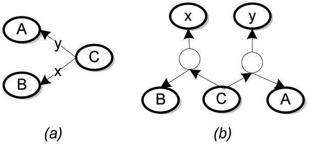
To facilitate graph matching, we may transform the edge-labeled graphs into unlabeled ones by elevating the edge labels to first class citizens of the graph. This process involves treating the relationships as resources, thereby adding them as nodes to the graph. We note that the transformation becomes unnecessary, from the perspective of ontology matching, when all edges have the same labels. We illustrate the transformation using a simple example in Fig. 1 and point out that the transformed graph is a bipartite graph (Hayes & Gutierrez, 2004). Consequently, the functions L_d in and L_m in become redundant.

Figure 1.

Transforming an edge labeled graph to a bipartite graph. (a) An edge labeled graph. (b) The transformed bipartite graph in which each distinct edge label is a node, and additional dummy nodes are introduced to preserve the relationships. The dummy nodes are null-labeled or may have identical labels.

However, this transformation into a bipartite graph comes at a price: The bipartite graph contains as many additional nodes as the number of edges and distinct edge labels. Because of this approximately two-fold increase in the number of nodes in the ontology, the transformation may be inappropriate for large ontologies with multiple edge labels. Consequently, we may consider matching the concept taxonomy and matching edge labels across ontologies as separate but dependent tasks.

4. Graph Matching Using GEM

As we mentioned previously, we model the ontology schemas as graphs, and , and consequently focus on the graph matching problem. While this perspective is not novel – for example, FALCON (Hu et al., 2005) also uses a graph-theoretic approach – we model the graph matching problem as a local search over the space of candidate matches and utilize the GEM iteratively to guide our search. GLUE (Doan et al., 2002) adopted a similar paradigm for ontology matching utilizing relaxation labeling iteratively for searching one-one maps. Because the best map is among the candidate matches, these approaches offer the potential of good performance.

Let M be a |V_d| × |V_m| matrix that represents the match between the two ontology graphs. In other words,

$$M=\left[\begin{array}{llll}{m}_{11}\hfill & m_{12}\hfill & \dots \hfill & m_{1\mid V_m\mid }\hfill \\ m_{21}\hfill & m_{22}\hfill & \dots \hfill & m_{2\mid V_m\mid }\hfill \\ .\hfill & .\hfill & \dots \hfill & .\hfill \\ .\hfill & .\hfill & \dots \hfill & .\hfill \\ .\hfill & .\hfill & \dots \hfill & .\hfill \\ m_{\mid V_d\mid 1}\hfill & m_{\mid V_d\mid 2}\hfill & \dots \hfill & m_{\mid V_d\mid \mid V_m\mid }\hfill \end{array}\right]$$

Within M, each assignment variable in the matrix is:

$$m_{a\alpha }=\{\begin{array}{ll}1\hfill & \text{if}f(x_a)=y_{\alpha }:x_a\in V_d,y_{\alpha }\in V_m\hfill \\ 0\hfill & \text{otherwise}\hfill \end{array}$$

where f is a map, f: V_d → V_m. We refer to an individual assignment of a model graph vertex, y_α, to a data graph vertex, x_a, by f, $x_a\stackrel{f}{\to }{y}_{\alpha }$, as a correspondence.

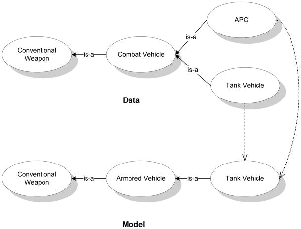
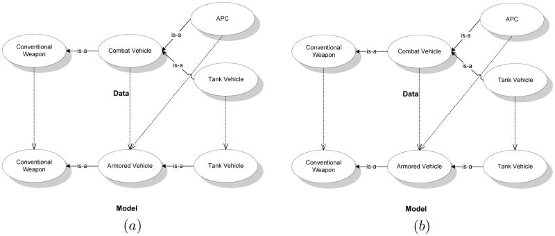
We illustrate the match matrix, M, using a simple example. We select small subsets of a pair of ontologies on Weapons, shown in Fig. 2, from the I³CON repository (Hughes & Ashpole, 2004) for the illustration. The matrix, M, for the example with the ordering of the nodes obtained by traversing the graphs from left to right is:

$$M=\left[\begin{array}{lll}0\hfill & 0\hfill & 0\hfill \\ 0\hfill & 0\hfill & 0\hfill \\ 0\hfill & 0\hfill & 1\hfill \\ 0\hfill & 0\hfill & 1\hfill \end{array}\right]$$

Figure 2.

Simple data and model ontology graphs with example map (shown using dashed arrows) for the purpose of illustration.

For a map, f, if {x_a, x_b}∈ E_d ⇔ {f(x_a), f(x_b)} ∈ E_m, then f is a homomorphism. We call the property of preserving edges across transformations as edge consistency. In this paper, we focus on tractably generating homomorphisms where f is a many-one map using the structural, lexical and instance based similarity between the participating ontologies to be matched. Our method may be generalized to finding many-many maps as well.

We formulate the graph matching as a maximum likelihood (ML) problem. Specifically, we are interested in the match matrix, M_*, that gives us the maximum conditional probability of the data graph, , given the model graph, and the match assignments. In other words, M_* is the match assignment that is most likely to generate given . Formally,

$$M_{\ast }=\underset{M\in \mathcal{M}}{\mathit{argmax}}Pr({\mathcal{O}}_d\mid {\mathcal{O}}_m,M)$$ (1)

where ℳ is the set of all match assignments. In general, there may be 2^|V_d||V_m| different matrices, but by restricting our focus to many-one maps we reduce the search space to (|V_m| + 1)^|V_d| (≪ 2^|V_d||V_m|). For the example in Fig. 2, the search space consists of 256 possible many-one maps compared to 4096 possible many-many maps. Of course, a better map may be found in those that are not considered. We note that the map may be partial: Some of the nodes in the data graph may not be mapped to any node in the model graph.

Given the model ontology we may assume the data graph nodes to be conditionally independent, and sum over the model graph nodes using the law of total probability.

$$\begin{array}{l}Pr({\mathcal{O}}_d\mid {\mathcal{O}}_m,M)=\prod _{x_a\in V_d}\sum _{y_{\alpha }\in V_m}Pr(x_a\mid y_{\alpha },M)Pr(y_{\alpha }\mid M)\\ =\prod _{x_a\in V_d}\sum _{y_{\alpha }\in V_m}Pr(x_a\mid y_{\alpha },M){\pi }_{\alpha }\end{array}$$

where π_α = Pr(y_α|M) is the prior probability of the model graph vertex, y_α, given the match matrix, M.

In order to solve the ML problem, we note that the map, f, is hidden from us. Additionally, if we view each assignment variable, m_aα, as a model, then the matrix M may be treated as a mixture model. Consequently, the mixture model, M, is parameterized by the set of the constituent assignment variables. Both these observations motivate the formulation of an EM technique to compute the mixture model with the maximum likelihood. We formulate the expectation (E) and the maximization (M) steps next.

4.1 E-Step

In order to compute the most likely map, we formulate a conditional expectation of the log likelihood with respect to the hidden variables given the data graph and a guess of the mixture model at some iteration n, Mⁿ.

$$Q(M^{n+1}\mid M^n)=E\left[\mathit{log}Pr(x_a\mid y_{\alpha },M^{n+1}){\pi }_{\alpha }^{n+1}\mid x_a,M^n\right]$$ (2)

The expectation in Eq. 2 may be rewritten as a weighted summation of the log likelihood with the weights being the posterior probabilities of the hidden correspondences under the matrix of assignment variables at iteration n. Equation 2 becomes:

$$Q(M^{n+1}\mid M^n)=\sum _{a=1}^{\mid V_d\mid }\sum _{\alpha =1}^{\mid V_m\mid }Pr(y_{\alpha }\mid x_a,M^n)\mathit{log}Pr(x_a\mid y_{\alpha },M^{n+1}){\pi }_{\alpha }^{n+1}$$

Expanding the log term, this may be rewritten as,

$$\begin{array}{l}Q(M^{n+1}\mid M^n)={\sum }_{a=1}^{\mid V_d\mid }{\sum }_{\alpha =1}^{\mid V_m\mid }Pr(y_{\alpha }\mid x_a,M^n)\mathit{log}Pr(x_a\mid y_{\alpha },M^{n+1})\\ +{\sum }_{a=1}^{\mid V_d\mid }{\sum }_{\alpha =1}^{\mid V_m\mid }Pr(y_{\alpha }\mid x_a,M^n)\mathit{log}{\pi }_{\alpha }^{n+1}\end{array}$$ (3)

Next, we address the computation of each of the terms in Eq. 3 by analyzing them further. We first focus on the posterior, Pr(y_α|x_a, Mⁿ). Once we establish a method for computing this term, the generation of log Pr(x_a|y_α, Mⁿ⁺¹) follows analogously.

Using Bayes theorem Pr(y_α|x_a, Mⁿ) may be rewritten,

$$Pr(y_{\alpha }\mid x_a,M^n)=\frac{Pr(x_a\mid y_{\alpha },M^n){\pi }_{\alpha }^n}{{\sum }_{\alpha =1}^{\mid V_m\mid }Pr(x_a\mid y_{\alpha },M^n){\pi }_{\alpha }^n}$$ (4)

where ${\pi }_{\alpha }^n=Pr(y_{\alpha }\mid M^n)$ is our guess of the prior which was defined previously.

We turn our attention to the term Pr(x_a|y_α, Mⁿ) in Eq. 4. This term represents the probability that the data graph node, x_a, is in correspondence with the model graph node, y_α, under the match matrix of iteration n, Mⁿ. Using Bayes theorem again,

$$\begin{array}{l}Pr(x_a\mid y_{\alpha },M^n)=\frac{Pr(x_a,y_{\alpha },M^n)}{Pr(y_{\alpha },M^n)}\\ =\frac{Pr(M^n\mid y_{\alpha },x_a)Pr(y_{\alpha },x_a)}{Pr(y_{\alpha },M^n)}\end{array}$$

As we mentioned before, Mⁿ is a mixture of the models, m_aα. We note that, in general, a correspondence between a particular pair of data and model nodes, say APC and Tank Vehicle in Fig. 2, need not always influence other correspondences, such as between the two Tank Vehicle nodes or even between Combat Vehicle and Armored Vehicle. Therefore, we treat the models in the matrix to be independent of each other. This allows us to write the above equation as,

$$Pr(x_a\mid y_{\alpha },M^n)=\frac{Pr(y_{\alpha },x_a){\mathrm{\Pi }}_{b=1}^{\mid V_d\mid }{\mathrm{\Pi }}_{\beta =1}^{\mid V_m\mid }Pr(m_{b\beta }^n\mid y_{\alpha },x_a)}{Pr(y_{\alpha }){\mathrm{\Pi }}_{b=1}^{\mid V_d\mid }{\mathrm{\Pi }}_{\beta =1}^{\mid V_m\mid }Pr(m_{b\beta }^n\mid y_{\alpha })}$$ (5)

We note that,

$$Pr(m_{b\beta }^n\mid y_{\alpha },x_a)=\frac{Pr(x_a\mid y_{\alpha },m_{b\beta }^n)Pr(m_{b\beta }^n\mid y_{\alpha })}{Pr(x_a\mid y_{\alpha })}$$

Substituting this into the numerator of Eq. 5 results in,

$$Pr(x_a\mid y_{\alpha },M^n)={[\frac{1}{Pr(x_a\mid y_{\alpha })}]}^{\mid V_d\mid \mid V_m\mid -1}{\mathrm{\Pi }}_{b=1}^{\mid V_d\mid }{\mathrm{\Pi }}_{\beta =1}^{\mid V_m\mid }Pr(x_a\mid y_{\alpha },m_{b\beta }^n)$$ (6)

We first focus on the term Pr(x_a|y_α, $m_{b\beta }^n$), which represents the probability that the node, x_a, in the data graph is in correspondence with y_α in the model graph given the assignment model, m_bβ. As we mentioned previously, m_bβ is 1 if x_b is in correspondence with y_β under the map f, otherwise it is 0. Let us call the set of nodes that are adjacent to x_a (linked by an edge) as its neighborhood, (x_a). For example, (Combat Vehicle) = {APC, Tank Vehicle} in the data graph. Since we seek f to be a homomorphism that must be edge consistent, for each vertex, x ∈ (x_a), the corresponding vertex, f(x) ∈ (y_α), if x_a is in correspondence with y_α. Therefore, the probability of x_a being in correspondence with y_α is dependent, in part, on whether the neighborhood of x_a is mapped to the neighborhood of y_α under f. Several approaches for schema matching (Milo & Zohar, 1998) and graph matching (Luo & Hancock, 2001) are based on this observation. To formalize this, we introduce the indicator variable, EC, which is defined as:

$$EC=\{\begin{array}{ll}1\hfill & \langle x_a,x_b\rangle \in E_d\wedge \langle y_{\alpha },y_{\beta }\rangle \in E_m\wedge m_{b\beta }=1\hfill \\ 0\hfill & \text{otherwise}\hfill \end{array}$$ (7)

In addition to the structural similarity, Pr(x_a|y_α, $m_{b\beta }^n$) is also influenced by the lexical similarity between the concept labels of the nodes x_a and y_α and by their instance based similarity. Taking the structural, lexical and instance based similarities into consideration we compute Pr(x_a|y_α, $m_{b\beta }^n$) as:

$$Pr(x_a\mid y_{\alpha },m_{b\beta }^n)={(1-P_{\epsilon }(x_a,y_{\alpha }))}^{EC}{P}_{\epsilon }{(x_a,y_{\alpha })}^{1-EC}$$ (8)

Here, P_ε: V_d × V_m → [0, 1] is the correspondence error based on the lexical similarity between node names (labels) and their instances. We address the computation of P_ε later in this article. Eq. 8 formalizes the intuition that the node Combat Vehicle is likely to be in correspondence with Armored Vehicle if the concept labels or their instances are lexically similar and say, the two Tank Vehicle nodes are matched. We note that Eq. 8 is a Bernoulli distribution and contrast it with the sigmoidal distribution that has been used previously (Tang, Li, Liang, Huang, Li, & Wang, 2006; Doan et al., 2002) to combine multiple match evidence.

In the term Pr(x_a|y_α) in Eq. 6, probability of node x_a is independent of y_α in the absence of the mixture model. Therefore, Pr(x_a|y_α) = Pr(x_a) whose value depends only on the identity of the node, x_a. In this article, we assume this distribution to be uniform, $Pr(x_a)=\frac{1}{\mid V_d\mid }$. We substitute Eq. 8 into Eq. 6 to obtain the following:

$$Pr(x_a\mid y_{\alpha },M^n)=\mid V_d{\mid }^{\mid V_d\left|\right|V_m\mid -1}{\mathrm{\Pi }}_{b=1}^{\mid V_d\mid }{\mathrm{\Pi }}_{\beta =1}^{\mid V_m\mid }{(1-P_{\epsilon }(x_a,y_{\alpha }))}^{EC}{P}_{\epsilon }{(x_a,y_{\alpha })}^{1-EC}$$ (9)

Substituting Eq. 9 into Eq. 4, we get,

$$Pr(y_{\alpha }\mid x_a,M^n)=C_a{\pi }_{\alpha }^n\mid V_d{\mid }^{\mid V_d\left|\right|V_m\mid -1}{\mathrm{\Pi }}_{b=1}^{\mid V_d\mid }{\mathrm{\Pi }}_{\beta =1}^{\mid V_m\mid }{(1-P_{\epsilon }(x_a,y_{\alpha }))}^{EC}{P}_{\epsilon }{(x_a,y_{\alpha })}^{1-EC}$$ (10)

where C_a is the normalizing constant and EC is as defined in Eq. 7.

We now look at the log likelihood term, log Pr(x_a|y_α, Mⁿ⁺¹), in Eq. 3. The computation of this term follows a similar path as before with the difference being that we use the new mixture model, Mⁿ⁺¹. Analogous to Eq. 6, we get,

$$\mathit{log}Pr(x_a\mid y_{\alpha },M^{n+1})=\mathit{log}\left[\mid V_d{\mid }^{\mid V_d\left|\right|V_m\mid -1}{\mathrm{\Pi }}_{b=1}^{\mid V_d\mid }{\mathrm{\Pi }}_{\beta =1}^{\mid V_m\mid }Pr(x_a\mid y_{\alpha },m_{b\beta }^{n+1})\right]$$

The presence of the log considerably simplifies the above.

$$\begin{array}{l}\mathit{log}Pr(x_a\mid y_{\alpha },M^{n+1})=(\mid V_d||V_m\mid -1)\mathit{log}\mid V_d\mid +\mathit{log}{\mathrm{\Pi }}_{b=1}^{\mid V_d\mid }{\mathrm{\Pi }}_{\beta =1}^{\mid V_m\mid }Pr(x_a\mid y_{\alpha },m_{b\beta }^{n+1})\\ =(\mid V_d||V_m\mid -1)\mathit{log}\mid V_d\mid +{\sum }_{b=1}^{\mid V_d\mid }{\sum }_{\beta =1}^{\mid V_m\mid }\mathit{log}Pr(x_a\mid y_{\alpha },m_{b\beta }^{n+1})\end{array}$$

The term Pr(x_a|y_α, $m_{b\beta }^{n+1}$) may be computed analogously to Eq. 8.

4.2 M-Step

The maximization step involves choosing the mixture model, $M_{\ast }^{n+1}$, that maximizes Q(Mⁿ⁺¹|Mⁿ), shown in Eq. 3. This mixture model then becomes the input for the next iteration of the E-step. However, the particular formulation of the E-step and the structure of the mixture model make it difficult to carry out the maximization analytically. Therefore, we relax the maximization requirement and settle for a mixture model, $M_{\ast }^{n+1}$, that simply improves the Q value. As we mentioned before in Section 2, this variant of the EM technique is called the generalized EM.

$$M_{\ast }^{n+1}=M^{n+1}\in \mathcal{M}:Q(M^{n+1}\mid M^n)\ge Q(M^n\mid M^n)$$ (11)

The priors, ${\pi }_{\alpha }^{n+1}$, for each α are those that maximize Eq. 3. We focus on maximizing the second term, ${\sum }_{\alpha =1}^{\mid V_m\mid }{\sum }_{a=1}^{\mid V_d\mid }Pr(y_{\alpha }\mid x_a,M^n)\mathit{log}{\pi }_{\alpha }^{n+1}$, of the equation, as the first term is independent of the prior. Differentiating it partially with respect to ${\pi }_{\alpha }^{n+1}$, and setting the resulting expression to zero results in,

$${\pi }_{\alpha }^{n+1}=\frac{1}{\mid V_d\mid }\sum _{a=1}^{\mid V_d\mid }Pr(y_{\alpha }\mid x_a,M^n)$$

The term Pr(y_α|x_a, Mⁿ) was computed previously in Eq. 4. We use ${\pi }_{\alpha }^{n+1}$ in the next iteration of the E-step.

4.3 Lexical Similarity Between Concepts Names and Instances

We compute the correspondence error, P_ε, between a pair of data graph and model graph nodes (Eq. 8) as one minus the maximum of the normalized lexical similarity between their respective labels and their instance based similarity.

Name based similarity

Under the umbrella of string distance, several metrics for computing the similarity between strings, such as n-grams, Jaccard, and sequence alignment exist (Cohen, Ravikumar, & Fienberg, 2003). We use the Smith-Waterman (SW) sequence alignment algorithm (Smith & Waterman, 1981) for calculating the lexical similarity between the node labels. In contrast to n-grams, the algorithm also takes into consideration non-contiguous sequences of characters that appear in the same order in both the labels, by assigning gap costs. The SW algorithm may be implemented as a fast dynamic program and requires a score for the similarity between two characters as the input. We assign a 1 if the two characters in consideration are identical and 0 otherwise. The algorithm generates the optimal local alignment by storing the maximum similarity between each pair of segments of the labels, and using it to compute the similarity between longer segments. For additional details and a detailed example, see (Smith & Waterman, 1981). We normalize the output of the SW algorithm by dividing it with the number of characters in the longer of the two labels. ¹

For illustration, let us consider the concept label “Missile Craft” that may appear in an ontology of weapons. The SW algorithm mentioned above assigns a score of 0.754 when aligned with the concept label “Missile Boat”, and a score of 0.477 when compared to the concept label “Torpedo Craft”, both of which may be found in another weapons ontology. In both cases, a contiguous, though different, sequence of characters match identically. Since a larger number of characters align exactly in the first case, a higher score is assigned to it.

Recently, several approaches to schema and ontology matching have used external sources such as WordNet (Miller, 1995) to additionally perform linguistic matches between the node labels (Do & Rahm, 2002; Giunchiglia, Shvaiko, & Yatskevich, 2004), that include considering synonyms, hypernyms and word senses. While these approaches may potentially discover better and semantic matches between the node labels, they rely on other external sources and incur associated computational overheads, which could be significant (Qu et al., 2006). Nevertheless, such approaches could easily be accommodated within our implementation to compute the correspondence error. For example, the lexical similarity between not only the node labels but also between their synonyms and hypernyms, obtained from WordNet, could be computed and the best similarity be used in computing the correspondence error. Investigating whether utilizing external sources, such as WordNet, is beneficial in comparison to the additional computational overhead is one line of our future work.

Restrictions, if present, provide more specific information about a concept by constraining properties defined for the concept. If restrictions are existential ( someValuesFrom in OWL) or universal ( allValuesFrom), and these are identical for the concepts whose correspondence is being considered, we use the lexical similarity as computed previously for the correspondence error. If these restrictions are not identical, we assign a high correspondence error. If node names are lexically similar but cardinality restrictions, if any, differ, we assign a high correspondence error. Otherwise, we do not consider these restrictions while computing the correspondence error.

Instance based similarity

We view each instance of a concept including the properties and their values as text. If an instance is a large document, we utilize word tokenization and stemming techniques and select tokens with high normalized frequencies and high inverse document frequencies if there are multiple documents. For each instance, we identify the corresponding one that is most similar. We compute the lexical similarity between the textual instances (or the representative tokens) of the pair of concepts as the average of such similarities across all instances. We utilize the SW algorithm mentioned previously to compute the lexical similarity. Analogous to text classification approaches as used in (Tang et al., 2006), we measure the similarity between the instances. While simpler, our approach is computationally efficient.

5. Illustration and Analysis of the EM

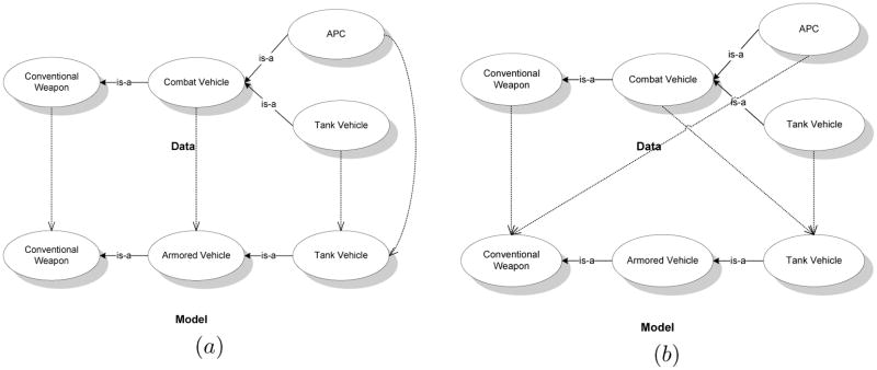
In order to better understand how Eqs. 3 to 8 help in calculating the quality of a match assignment between the nodes of two ontologies, we illustrate an iteration of the E-step using a simple example. We utilize the simple ontology graphs introduced in Fig. 2 for the illustration. We pick two candidate matches between the ontologies, $M_1^1$ and $M_2^1$ (Fig. 4), and show the corresponding Q-values (Eq. 3) using an initial seed match, M⁰. Among the two candidate matches, $M_2^1$ is obviously a poor match compared to $M_1^1$ as it is not edge consistent, and we demonstrate that $Q(M_1^1\mid M^0)>Q(M_2^1\mid M^0)$, which reflects this fact. Using more refined examples, we then proceed to demonstrate some interesting features of our approach.

Figure 4.

Two candidate matches, $M_1^1$ and $M_2^1$, between the example ontologies. The first one is a better match than the second.

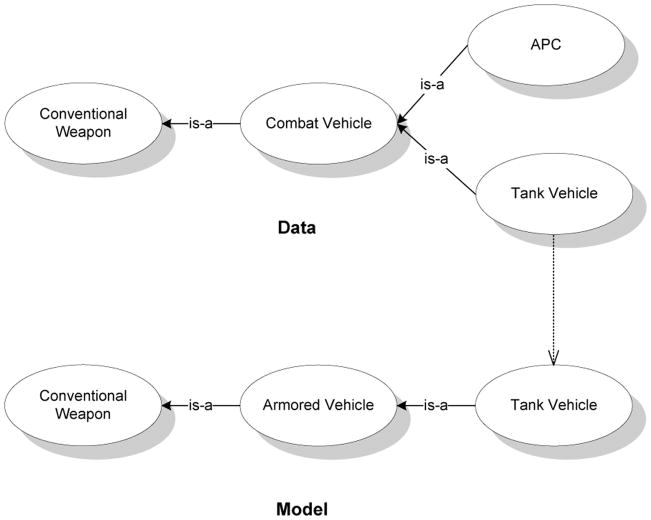
We show M⁰ in Fig. 3 in which the concepts Tank Vehicle of the data and model ontologies are matched. Before we illustrate the computations in the E-step, we give the correspondence error, P_ε, between the node labels in Table 1. The values were calculated using the SW technique mentioned in Section 4.3.

Figure 3.

The seed match, M⁰, between the example ontologies. The concepts Tank Vehicle of the two ontologies are matched. Notice that the data ontology has an “extra” node.

Table 1.

The correspondence errors between the node labels of the data (row) and model (column) ontologies. Large values indicate high errors and low lexical similarities. We avoid zero values to prevent division-by-zero situations.

Node Labels	“Tank Vehicle”	“Armored Vehicle”	“Conventional Weapon”
“Tank Vehicle”	0.0001	0.4667	0.80
“Combat Vehicle”	0.4143	0.4133	0.768
“Conventional Weapon”	0.8	0.8316	0.0001
“APC”	0.9983	0.9933	0.9947

We begin by evaluating $Q(M_1^1\mid M^0)$ where $M_1^1$ is as shown in Fig. 4(a) and represented using the matrix given below. The order of the nodes of the data ontology along the rows and those of the model ontology along the columns is identical to Table 1.

$$M_1^1=\left[\begin{array}{lll}1\hfill & 0\hfill & 0\hfill \\ 0\hfill & 1\hfill & 0\hfill \\ 0\hfill & 0\hfill & 1\hfill \\ 1\hfill & 0\hfill & 0\hfill \end{array}\right]$$

In order to calculate $Q(M_1^1\mid M^0)$, we focus on the first term of Eq. 3 since the second term is independent of $M_1^1$. We evaluate the term, Pr(y_α|x_a, M⁰) logPr(x_a|y_α, $M_1^1$), for each combination of nodes from the data and model ontologies. In order to evaluate this term, we first focus on calculating Pr(y_α|x_a, M⁰) using Eq. 10. This, in turn, requires the calculation of Pr(x_a|y_α, M⁰) according to Eq. 9. We pick the node APC from the data ontology and iterate over all nodes in the model ontology in order to illustrate the calculations:

Pr(x_a = APC|y_α = Tank Vehicle, M⁰) = 4¹¹ × 0.9983¹² = 4.11 × 10⁶

Pr(x_a = APC|y_α = Armored Vehicle, M⁰) = 4¹¹ × 0.9933¹² = 3.87 × 10⁶

Pr(x_a = APC|y_α = Conventional Weapon, M⁰) = 4¹¹ × 0.9947¹² = 3.98 × 10⁶

Next, we calculate C_a, the normalizing constant in Eq. 10. $C_a=\frac{1}{{\sum }_{\alpha =1}^{\mid V_m\mid }Pr(x_a=\mathit{APC}\mid y_{\alpha },M^0){\pi }_{\alpha }^0}=\frac{1}{1.196\times {10}^7\times 0.33}=2.53\times {10}^{-7}$, where ${\pi }_{\alpha }^0=\frac{1}{\mid V_m\mid }$

We may now calculate Pr(y_α|x_a, M⁰) for the combinations of APC in the data graph and each node in the model graph.

Pr(y_α = Tank Vehicle|x_a = APC, M⁰) = 2.53 × 10⁻⁷ × 0.33 × 4.11 × 106 = 0.34

Pr(y_α = Armored Vehicle|x_a = APC, M⁰) = 2.53 × 10⁻⁷ × 0.33 × 3.87 × 106 = 0.32

Pr(y_α = Conventional Weapon|x_a = APC, M⁰) = 2.53 × 10⁻⁷ × 0.33 × 3.98 × 106 = 0.33

The remaining term, log Pr(x_a|y_α, $M_1^1$), in Eq. 3 is as follows:

ln Pr(x_a = APC|y_α = Tank Vehicle, $M_1^1$) = 15.23

ln Pr(x_a = APC|y_α = Armored Vehicle, $M_1^1$) = 15.17

ln Pr(x_a = APC|y_α = Conventional Weapon, $M_1^1$) = 15.19

We denote the first term of Eq. 3 for the data node, APC, as ℱ_APC, and its value is as follows:

$$\begin{array}{l}{\mathcal{F}}_{\mathit{APC}}={\sum }_{\alpha =1}^{\mid V_m\mid }Pr(y_{\alpha }\mid x_a=\mathit{APC},M^0)\mathit{lnPr}(x_a=\mathit{APC}\mid y_{\alpha },M_1^1)=0.34\times 15.23+0.32\times \\ 15.17+0.33\times 15.19=15.05\end{array}$$

Analogous calculations are carried out to compute ℱ_{Tank Vehicle}, ℱ_{Combat Vehicle}, and ℱ_{Conventional Weapon}, resulting in the following values:

ℱ_{Tank Vehicle} = 12.578,

ℱ_{Combat Vehicle} = 12.07, and

ℱ_{Conventional Weapon} = 12.86

We may calculate the first term of $Q(M_1^1\mid M^0)$ as,

$$\begin{array}{l}Q(M_1^1\mid M^0{)}^{\prime }={\mathcal{F}}_{\mathit{APC}}+{\mathcal{F}}_{\mathit{TankVehicle}}+{\mathcal{F}}_{\mathit{CombatVehicle}}+{\mathcal{F}}_{\mathit{ConventionalWeapon}}\\ =\mathbf{52}.\mathbf{56}\end{array}$$

We proceed to the next candidate match, $M_2^1$, shown in Fig. 4(b), and evaluate the first term of $Q(M_2^1\mid M^0)$. The matrix form of $M_2^1$ is shown below.

$$M_2^1=\left[\begin{array}{lll}1\hfill & 0\hfill & 0\hfill \\ 1\hfill & 0\hfill & 0\hfill \\ 0\hfill & 0\hfill & 1\hfill \\ 0\hfill & 0\hfill & 1\hfill \end{array}\right]$$

Performing analogous calculations as above, we obtain the following values for ℱ_APC, ℱ_{Tank Vehicle}, ℱ_{Combat Vehicle}, and ℱ_{Conventional Weapon}:

ℱ_APC = 15.05,

ℱ_{Tank Vehicle} = 12.578,

ℱ_{Combat Vehicle} = 12.06, and

ℱ_{Conventional Weapon} = 11.88

Intuitively, ℱ_APC and ℱ_{Tank Vehicle} remain unchanged because both, APC and Tank Vehicle, are leaf nodes. However, there is a slight reduction in the value of ℱ_{Combat Vehicle} because its neighbor, APC, is not matched with Tank Vehicle, as in $M_1^1$. The maximum change is in the value of ℱ_{Conventional Weapon} because the neighbors of Conventional Weapon in the two ontologies are not matched, and Combat Vehicle matched with Tank Vehicle suggests that matching Conventional Weapon with Armored Vehicle may be a map structurally.

$Q(M_2^1\mid M^0{)}^{\prime }$ is 51.57, which is less than $Q(M_1^1\mid M^0{)}^{\prime }$ thereby suggesting that in comparison to $M_1^1$, the match, $M_2^1$, is worse.

Next, we compare $M_1^1$ with a match, $M_3^1$, that greedily aligns concepts that lexically are most similar (see Fig. 5(a)). In addition to aligning identically labeled concepts, Combat Vehicle in the data graph is mapped to Armored Vehicle in the model graph and APC is mapped to Armored Vehicle as well. $Q(M_3^1\mid M^0{)}^{\prime }$ is 52.41 which is lower compared to $Q(M_1^1\mid M^0{)}^{\prime }$ indicating that $M_3^1$ is deemed a worse match. The difference between the two Q-values is small as only a single correspondence – APC to Armored Vehicle – differentiates the two matches. This also indicates that our approach is able to trade off lexical similarity for structural consistency.

Figure 5.

Candidate (a) represents a greedy match that maps nodes with the largest string similarity. Match (b) is a one-one map between the two ontologies, included here for comparison with the many-one map. Match (b) is preferred over (a).

We further compare $M_1^1$ with another match, $M_4^1$ shown in Fig. 5(b), in order to demonstrate the need for a many-one map. $M_4^1$ is a one-one map that, in addition to mapping identically labeled concepts also maps Combat Vehicle to Armored Vehicle; APC is not mapped to any node in the model graph. $Q(M_4^1\mid M^0{)}^{\prime }$ is 52.42 indicating that in comparison to $M_4^1$ the more accurate map, $M_1^1$, is preferred, which maps APC to Tank Vehicle in the model graph. This is because the map from APC to Tank Vehicle in $M_1^1$ further reinforces the likelihood of the map from Combat Vehicle to Armored Vehicle. Note that $M_4^1$ is preferred over $M_3^1$ indicating that a one-one map with correct correspondences is preferable to a many-one map with an incorrect correspondence. This indicates that our approach may settle for a one-one map if it is deemed more likely.

Finally, we compare $M_1^1$ with a match, $M_5^1$, that maps only the identically labeled concepts. $Q(M_5^1\mid M^0{)}^{\prime }$ is 45.51 indicating its poor quality. Although, the Conventional Weapon concepts are mapped, the absence of a correspondence between Combat Vehicle and Armored Vehicle somewhat contradicts that map, and contributes to the difference in Q-value.

These examples demonstrate that the Q-values as calculated by the E-step serve as reliable indicators of the goodness of a match between two ontologies. A limitation of relying, in part, on structural similarity to identify a many-one map is that an additional concept that is a subclass of Combat Vehicle in the data graph such as Fighter Aircraft would also be aligned with Tank Vehicle. In the absence of domain knowledge, we believe that it is difficult to avoid such matches. As lexical and structural similarities between independently developed ontologies often conflict, our approach effectively balances the two in discovering a map.

6. Random Sampling with Local Improvements

In this section, we present a way of arriving at the mixture model, $M_{\ast }^{n+1}$, that satisfies the inequality in Eq. 11. We observe that an exhaustive search of the complete model space is infeasible due to its large size – there are (|V_m| + 1)^|V_d| many distinct mixture models. On the other hand, both the EM and its generalization, GEM, are known to often converge to the local maxima (Dempster et al., 1977) (instead of the global) when the search space for selecting $M_{\ast }^{n+1}$ is parsimonious. This suggests that any technique for generating $M_{\ast }^{n+1}$ should attempt to cover as much of the model space as possible, while maintaining tractability.

A straightforward approach for generating $M_{\ast }^{n+1}$ is to randomly sample K mixture models, ℳ̂ = {M⁽¹⁾, M⁽²⁾, ···, M^(K)}, and select the one as $M_{\ast }^{n+1}$ that satisfies the constraint in Eq. 11. If more than one satisfy the inequality, then we pick the one with the higher Q-value and break ties randomly. We sample the models by assuming a flat distribution over the model space. The set of samples, ℳ̂, may be seen as a representative of the complete model space. However, since there is no guarantee that a sample within the sample set will satisfy the constraint in Eq. 11, we may have to sample several ℳ̂, before a suitable mixture model is found. This problem becomes especially severe when the model space is large and a relatively small number of samples, K, is used. Faced with a somewhat similar situation though in a different context, Dhamankar et al. (Dhamankar et al., 2004) utilized beam search with a beam width of K that retained only the best K matches, for searching over a very large space of candidate matches.

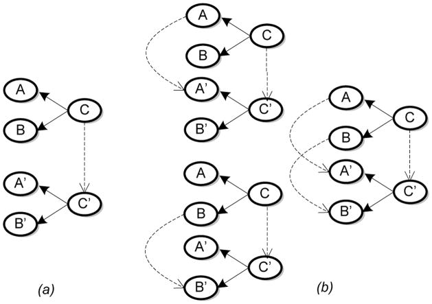
In order to reduce the number of ℳ̂s that are discarded, we exploit intuitive heuristics that guide the generation of Mⁿ⁺¹. For taxonomies in particular, if Mⁿ exhibits correspondences between some subclasses in the two graphs, then match their respective parents, to generate a candidate Mⁿ⁺¹. For the case where a subclass has more than one parent, lexical similarity is used to resolve the conflict. We illustrate this heuristic in Fig. 6. This and other general and domain-specific heuristics have been used previously in (Doan et al., 2002; Mitra et al., 2004) where they were shown to be effective.

Figure 6.

An example application of the heuristic – if at least one pair of subclasses is matched, then match the respective parents. The nodes are concepts and edges in the graphs denote the rdfs:subClassOf relationship. (a) Mⁿ – the dashed arrow shows the match between the two subclasses C and C′. (b) Three candidate Mⁿ⁺¹s with parents matched according to lexical similarity.

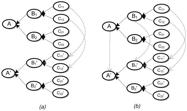
However, a simple example, Fig. 7, demonstrates that solely utilizing such a heuristic is insufficient to generate all the correspondences. In particular, the performance of the heuristic is dependent on the initial correspondences that are provided. To minimize the convergence to local maximas, we augment the set of heuristically generated mixture models with those that are randomly sampled. In this manner, not only do we select candidate mixture models that have a better chance of satisfying Eq. 11, but we also cover the model space. This approach is analogous to the technique of random restarts, commonly used to dislodge hill climbing algorithms that have converged to local maximas.

Figure 7.

An illustration of the correspondences generated by the heuristic. (a) Mⁿ (b) Correspondences after multiple applications of the heuristic. Unless we combine the heuristic with others or randomly generated correspondences, no more correspondences can be generated and a local maxima is reached.

7. Computational Complexity

We first analyze the complexity of computing Q(Mⁿ⁺¹|Mⁿ) which forms the E-step. From Eq. 10, the complexity of the posterior, Pr(y_α|x_a, Mⁿ), is a combination of the complexity of computing EC |V_d||V_m| times, the correspondence error (P_ε), and the term ${[\frac{1}{\mid V_d\mid }]}^{\mid V_d\left|\right|V_m\mid -1}$. We observe that EC may be computed through a series of look-up operations, and is therefore of constant time complexity. The complexity of calculating P_ε, dependent on the algorithm for arriving at the lexical similarity, is O(l²) for the SW technique, where l is the length of the largest concept label. If instances are present, l is the length of the largest instance. The complexity of the exponential term is O(log₂|V_d||V_m| − 1). Hence the computational complexity of the posterior is O(log₂|V_d||V_m| − 1) + O(|V_d||V_m|) + O(l²) = O(|V_d||V_m|). The computational complexity of the log likelihood term is also O(|V_d||V_m|), because its computation proceeds analogously. Since the product of these terms is summed over |V_d||V_m|, the final complexity of the E-step is O([|V_d||V_m|]²). In the M-step, if we generate K samples within a sample set, the worst case complexity is O(K[|V_d||V_m|]²). For edge-labeled graphs, the complexity of the transformation into a bipartite graph is O(|E|log₂|E|) where |E| is the number of edges in the graph.

8. Initial Experiments

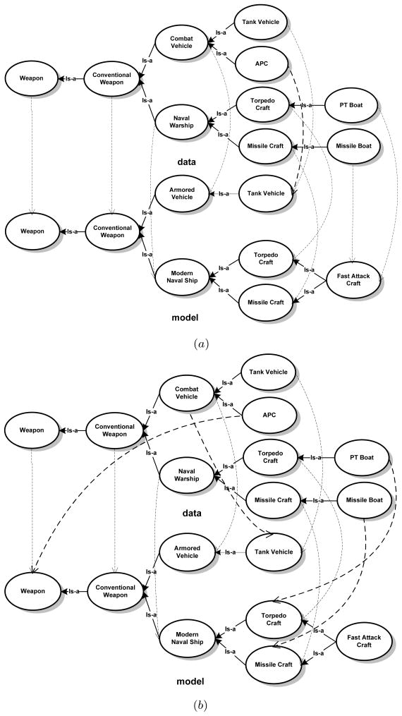
We analyze the performance of our methods on example ontology pairs obtained from the I³CON benchmark repository (Hughes & Ashpole, 2004). The repository contains pairs of ontologies on identical domains but derived from different sources. The ontologies that we use are expressed in the N3 language (Berners-Lee, 2000) – an experimental non-XML notation for encoding ontologies. While a good match accuracy is of utmost importance, we also focus on the computational resources consumed in arriving at the match. We utilize a partial subset of the Weapons ontologies with slight modifications for a detailed analysis of our methods. In particular, our modifications include adding the concept of PT Boat in the data ontology, Fast Attack Craft in the model ontology, and adding the associated edges. A many-one map, not required by the original subsets, is made possible by these modifications. The modified pair thus serves as a test for an approach capable of discovering such matches. In Fig. 8(a) we show the match produced by the GEM algorithm. We utilized the random sampling combined with heuristic improvement to generate Mⁿ⁺¹ at each step of the iteration. In order to illustrate the need for considering graph structure while matching, we also show the match obtained by using just the lexical similarity between concept labels (Fig. 8(b)). We calculate the recall and precision as follows:

$$\begin{array}{l}\text{recall}=\frac{\text{No}.\text{of}\text{correctly}\text{identified}\text{correspondences}}{\text{Total}\text{no}.\text{of}\text{correct correspondences}}\\ \text{precision}=\frac{\text{No}.\text{of}\text{correctly}\text{identified}\text{correspondences}}{\text{Total}\text{no}.\text{of}\text{identified}\text{correspondences}}\end{array}$$ (12)

Figure 8.

Utility of considering structure while matching. (a) The correspondences generated by our GEM method (recall (in percentage): 100%; precision (in percentage): 90% – 1 false-positive). (b) Correspondences generated using only the string similarity between concept labels (recall: 77.8%; precision: 63.6%). The dashed arrows in bold are the incorrect matches.

Thus, while recall is a good measure of the match accuracy, precision indicates the percentage of false positives.

We point out that the many-one homomorphism in Fig. 8(a) mapped both PT Boat and Missile Boat nodes of the data graph to the Fast Attack Craft node of the model graph. This illustrates a subsumption match because the former concepts are encompassed by the latter. Further, if the node Torpedo Craft in the model ontology is replaced with Destroyer – lexically less similar to “Torpedo Craft”– then the map in which Torpedo Craft and PT Boat do not correspond to any node in the model ontology is preferred to, (a) a map in which PT Boat corresponds to Fast Attack Craft and Torpedo Craft in data graph to Destroyer and, (b) a map in which PT Boat corresponds to Fast Attack Craft and Torpedo Craft to Missile Craft. Thus, lexical similarity between concept names also guides the map and an edge consistent map of maximum cardinality is not always preferred.

In Fig. 9(a) we show the performance (recall) profile of the GEM with random sampling. It is straightforward to see that the precision in our experiments will be greater than or equal to 0.9 times the recall. Specifically, as each Mⁿ⁺¹ is limited to a many-one map, no node of the data graph may appear more than once in the correspondences. Hence, as there are at most 10 correspondences in any map and the total number of correct correspondences are 9, the relation between recall and precision follows. Each data point in the plots is an average of 10 independent runs, and our seed mixture model (M⁰) contained a single match between the Tank Vehicle nodes of both ontologies. As we increase the size of the sample sets (from 100 to 1,000 samples), we obtain a greater recall at each iteration. This is because a larger percentage of the complete search space (≈ 10⁹ distinct many-one maps) is covered. However, from Table 2, we observe that the running time over all the iterations also increases as the sample size increases. To measure the effectiveness of random sampling, we also provide the total number of sample sets, ℳ̂, that were generated over all the iterations. For 100 samples, an average of 57 sample sets per iteration were generated before a satisficing Mⁿ⁺¹ was found, while an average of 38 sample sets were used per iteration for 1,000 samples. On including the heuristic (Fig. 6) in addition to random sampling during the optimization step, we obtain the performance profiles shown in Fig. 9(b). The heuristic not only improves the recall but also significantly reduces the number of sample sets generated and therefore the time consumed in performing the iterations (Table 2). While smaller size sample sets lead to local maximas, sets of 5,000 samples produced 90%–100% recall for all the runs. We observe that the heuristic by itself is not sufficient: starting from our seed model, employing just the heuristic for the optimization step leads to only a 40% recall.

Figure 9.

Performance profiles of the GEM method on Weapons ontologies. (a) Random sampling was used for generating the next Mⁿ⁺¹. (b) A combination of heuristic and random sampling is used for generating Mⁿ⁺¹.

Table 2.

The total running times (JDK 1.5 program on a dual processor Xeon 3.4GHz, 4GB RAM, and Linux) and sample sets generated over all the iterations.

Method	Metric	K=100	K=500
Random	Time	3m 39.29s ± 4m 19.09s	19m 26.46s ± 19m 24.5s
sampling	Sample sets	570 ± 666	373 ± 368
Sampling with	Time	10.3s ± 1.7s	48.12 ± 11.2s
local improvements	Sample sets	26 ± 5	25 ± 6
Method	Metric	K=1000	K=5000
Random	Time	23m 25s ± 16m 42.63s	*
sampling	Sample sets	376 ± 264	*
Sampling with	Time	1m 50.6s ± 24.11s	8m 41.3s ± 1m 22.46s
local improvements	Sample sets	27 ± 6	27 ± 4

^*= program ran out of memory

In order to judge the performance of our method on more complex ontologies, we tested it on larger subsets of the Weapons ontologies, rooted at Conventional Weapons, and subsets of the Network ontologies. The data and model graphs for Weapons contained 22 and 19 nodes, respectively. The GEM method combined with heuristically and randomly generated samples converged to a match with a recall of 100% and a precision of 86.4% in 17m 47.2s with a seed model of 10% accurate matches. The run time is halved if we settle for a slightly lower recall (90%) by reducing the number of samples. The Network ontologies, in addition to containing more nodes, exhibit labeled relationships. After transforming the ontology graphs into bipartite graphs using the procedure illustrated in Fig. 1, both the data and model graphs contained 19 nodes and 24 edges each. The GEM method converged to a match with a recall and precision of 100% in 10m 53.1s with a seed model of 10% accuracy.

In summary, our initial empirical investigation indicates that the approach performs well as is evident from the high recall values for the different ontology pairs. Though the somewhat high run times are due to the way we perform the maximization step, computational bottlenecks exist that affect its applicability to larger ontologies. We address these challenges next.

9. Matching Large Ontologies Using Memory Bounded Partitioning

The experimental results in Section 8 illustrate the accuracy of the approach, but also highlight its inability to match large ontologies – those containing several hundreds of concepts. We identify two reasons why the approach does not scale well to larger tasks.

First, within the E-step, the computation of the term, Q(Mⁿ⁺¹|Mⁿ), as shown in Eq. 3 requires iterating over all the model and data graph nodes, and computing the weighted log likelihood. Consequently, both the ontologies need to be entirely stored in main memory to facilitate the computation. For large ontologies, this becomes a computational bottleneck. Second, the exponential term, |V_d|^{|V_d||V_m|−1}, in Eq. 6 causes the computed value to become unmanageably large (often causing overflows) for ontologies with several nodes.

In order to address these difficulties, we partition each of the two ontologies to be matched. Let and be the partitions of the set of data and model graph vertices (including nodes in the transformed bipartite graphs), respectively. We denote each non-empty disjoint subset of V_d within the partition as ${\mathcal{V}}_d^i$, where i = 1 … ||, and analogously for the model graph. Because iterating over all the graph nodes is equivalent to iterating over all the partitions and over all nodes within a partition, Eq. 3 may be decomposed into:

$$\begin{array}{l}Q(M^{n+1}\mid M^n)={\sum }_{i=1}^{\mid {\mathcal{P}}_d\mid }{\sum }_{a=1}^{\mid {\mathcal{V}}_d^i\mid }{\sum }_{j=1}^{\mid {\mathcal{P}}_m\mid }{\sum }_{\alpha =1}^{\mid {\mathcal{V}}_m^j\mid }Pr(y_{\alpha }\mid x_a,M^n)\mathit{logPr}(x_a\mid y_{\alpha },M^{n+1})\\ +{\sum }_{i=1}^{\mid {\mathcal{P}}_d\mid }{\sum }_{a=1}^{\mid {\mathcal{V}}_d^i\mid }{\sum }_{j=1}^{\mid {\mathcal{P}}_m\mid }{\sum }_{\alpha =1}^{\mid {\mathcal{V}}_m^j\mid }Pr(y_{\alpha }\mid x_a,M^n)\mathit{log}{\pi }_{\alpha }^{n+1}\end{array}$$

A simple rearrangement of the summations yields the following:

$$\begin{array}{l}Q(M^{n+1}\mid M^n)={\sum }_{i=1}^{\mid {\mathcal{P}}_d\mid }{\sum }_{j=1}^{\mid {\mathcal{P}}_m\mid }\left({\sum }_{a=1}^{\mid {\mathcal{V}}_d^i\mid }{\sum }_{\alpha =1}^{\mid {\mathcal{V}}_m^j\mid }Pr(y_{\alpha }\mid x_a,M^n)\mathit{logPr}(x_a\mid y_{\alpha },M^{n+1})\right)\\ +{\sum }_{i=1}^{\mid {\mathcal{P}}_d\mid }{\sum }_{j=1}^{\mid {\mathcal{P}}_m\mid }\left({\sum }_{a=1}^{\mid {\mathcal{V}}_d^i\mid }{\sum }_{\alpha =1}^{\mid {\mathcal{V}}_m^j\mid }Pr(y_{\alpha }\mid x_a,M^n)\mathit{log}{\pi }_{\alpha }^{n+1}\right)\end{array}$$ (13)

Notice that the terms within the parenthesis are analogous to the terms in Eq. 3, except that we now sum over all nodes in a subset within the partition.

One simple way to partition an ontology graph is to traverse the graph in a breadth-first manner² starting from a root node and collect MB number of nodes within a subset. Here, 2 × MB is the total number of nodes that can be held in main memory at any given time. The resulting disjoint sets of nodes collectively form a partition over the set of ontology nodes. ³ We label a node within an ontology as root if it has no outgoing arcs. While taxonomies, by definition, contain a root node, ontologies in general may not. In the absence of a root node, we may create one by selecting a node with the lowest number of outgoing arcs and connecting it to a dummy root node. This node, for example, could denote the rdfs:Thing class within the RDF schema, which generalizes all classes in RDF. Of course, other approaches for traversing and partitioning an ontology graph also exist with varying computational overheads (for example, see Stuckenschmidt & Klein, 2004). Whether these approaches result in partitions that better facilitate matching is an aspect of our future investigations.

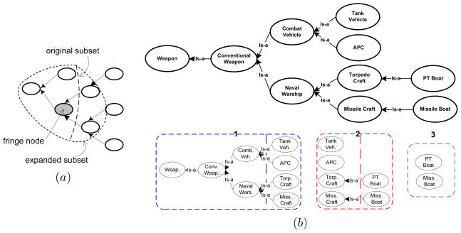
Equation 13 helps alleviate the difficulty of insufficient memory for large ontologies by requiring that only the nodes within a subset of the partition be held in memory for log likelihood computations. However, this approach does not address the problem of having to compute large exponents, referred to previously. In order to address this, we observe that in computing EC (Eq. 7), we utilize only the nodes within the ontology graphs that are in the immediate neighborhood of the nodes in consideration for matching. This simple insight allows us to replace the mixture models, Mⁿ and Mⁿ⁺¹, used in the computation of the weighted log likelihood with the following: if ${\mathcal{V}}_d^i$ is a subset within the partition of the data graph nodes, let ${\mathcal{V}}_d^{i,+}$ be the expanded set that additionally includes all nodes (belonging to V_d) that are the immediate neighbors of the nodes in ${\mathcal{V}}_d^i$. This involves identifying the fringe or boundary nodes in ${\mathcal{V}}_d^i$ and including their immediate neighbors (Fig. 10). Let ${\mathcal{V}}_m^{j,+}$ be the analogously expanded set of nodes for the subset ${\mathcal{V}}_m^j$. Then, define $M_{ij}^n$ to be that region (sub-matrix) of Mⁿ, which consists of the nodes in ${\mathcal{V}}_d^{i,+}$ as rows, and the nodes in ${\mathcal{V}}_m^{j,+}$ as columns of the sub-matrix, and analogously for $M_{ij}^{n+1}$.

Figure 10.

(a) The original subset consists of the nodes to be matched. The subset is expanded to include the neighboring nodes of the fringe or boundary nodes in the original subset. Note that the newly included nodes are not considered for mapping. (b) A partition of the Weapons ontology shown previously in Section 8. For illustration, MB = 4, due to which three parts are identified. In the first two parts, fringe nodes are shown included. Each part is compared for mapping with another of the target ontology.

In Eq. 13, we replace the mixture models in the computation of the weighted log likelihood with the partial ones. This transforms Eq. 13 into the following:

$$\begin{array}{l}{Q}^{\prime }(M^{n+1}\mid M^n)={\sum }_{i=1}^{\mid {\mathcal{P}}_d\mid }{\sum }_{j=1}^{\mid {\mathcal{P}}_m\mid }\left({\sum }_{a=1}^{\mid {\mathcal{V}}_d^i\mid }{\sum }_{\alpha =1}^{\mid {\mathcal{V}}_m^j\mid }Pr(y_{\alpha }\mid x_a,M_{ij}^n)\mathit{logPr}(x_a\mid y_{\alpha },M_{ij}^{n+1})\right)\\ +{\sum }_{i=1}^{\mid {\mathcal{P}}_d\mid }{\sum }_{j=1}^{\mid {\mathcal{P}}_m\mid }\left({\sum }_{a=1}^{\mid {\mathcal{V}}_d^i\mid }{\sum }_{\alpha =1}^{\mid {\mathcal{V}}_m^j\mid }Pr(y_{\alpha }\mid x_a,M_{ij}^n)\mathit{log}{\pi }_{\alpha }^{n+1}\right)\end{array}$$ (14)

While this modification will not affect Eq. 8, the exponential term |V_d|^{|V_d||V_m|−1} in Eq. 6 becomes $\mid {\mathcal{V}}_d^{i,+}{\mid }^{\mid {\mathcal{V}}_d^{i,+}\left|\right|{\mathcal{V}}_m^{j,+}\mid -1}$, as we show below. For large ontologies, this is likely to be much less than the former.

$$Pr(x_a\mid y_{\alpha },{\mathcal{M}}_{ij}^n)=\mid {\mathcal{V}}_d^{i,+}{\mid }^{\mid {\mathcal{V}}_d^{i,+}\left|\right|{\mathcal{V}}_m^{j,+}\mid -1}{\mathrm{\Pi }}_{b=1}^{\mid {\mathcal{V}}_d^{i,+}\mid }{\mathrm{\Pi }}_{\beta =1}^{\mid {\mathcal{V}}_m^{j,+}\mid }Pr(x_a\mid y_{\alpha },m_{b\beta }^n)$$ (15)

Althought the right hand side of Eq. 14 is no longer equivalent to that of Eq. 13 because of the changed exponential term, the property that high Q-values indicate better matches is preserved.

To summarize, we modify the GEM in the following way so as to enable matching of larger ontologies:

1. Partition the data and model ontology graphs where the number of nodes within any subset in the partitions does not exceed MB. Here, 2 × MB is the total number of nodes that can be held in memory.

2. Expand each of the subsets within the partitions to include the immediate neighbors of the original nodes in the subset.

3. Perform the E-step using Eq. 14 where partial regions of the mixture models are used to compute the weighted log likelihoods.

10. Experiments on Benchmark Sets

We evaluated the performance of the GEM algorithm modified using the memory-bounded partitioning scheme on two well-known benchmark sets for evaluating ontology alignment algorithms. The first benchmark set is the previously mentioned I³CON repository (Hughes & Ashpole, 2004) from which we selected six ontology pairs and the corresponding true maps for evaluation. We list these pairs along with the associated statistics such as the number of concepts, relationships (edge labels) and the depth of the hierarchies in the ontologies, in Table 3.

Table 3.

Ontology pairs used for evaluation from the I³CON repository and some associated statistics.

Ontology pair	No. of concepts	No. of relationships	Max. depth
Wine A & B	33 & 33	1 & 1	2 & 2
Weapons A & B	63 & 58	1 & 1	4 & 5
Network A & B	28 & 28	6 & 7	3 & 3
CS A & B	109 & 20	52 & 7	6 & 4
People+Pets A & B	60 & 58	15 & 15	4 & 3
Russia A & B	158 & 150	81 & 76	6 & 8

Of the ontology pairs listed in Table 3, the pair labeled Russia A & B consists of the largest ontology graphs with 158 and 150 nodes, respectively, which are related to each other using 81 and 76 edge labels, respectively. These ontologies partially describe the culture, places of interest, infrastructure and jobs in the country of Russia. We also point out the CS ontology pair because of its dissimilarity – one member of the pair contains 109 nodes and 52 edge labels, while the other contains 20 nodes and 7 edge labels. These ontologies describe the social organization, infrastructure and functions of a typical computer science department, though at widely varying granularities.

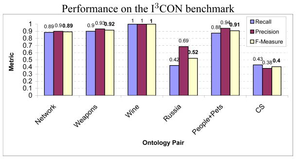
We show the performance of our matching algorithm on the ontology pairs in Fig. 11. The recall and precision of the maps were calculated according to Eq. 12, the F-measure was calculated as: $\text{F}-\text{measure}=2\times \frac{\text{Recall}\times \text{Precision}}{\text{Recall}+\text{Precision}}$. The seed maps consisted of mapping 5% to 10% of the leaf nodes or correspondences obtained by matching node labels exactly. We observe that the performance on the CS and Russia ontologies is weak. This is because the CS ontologies exhibit large structural dissimilarities, as is evident from their respective sizes shown in Table 3. Though the Russia pair of ontologies have approximately similar number of nodes and edge labels, their internal graph structure as well as the node labels are largely dissimilar leading to a low level of performance. On the other hand, our algorithm perfectly matched the Wine pair of ontologies and demonstrated satisfactory performance on the other pairs.

Figure 11.

Recall, precision and F-measure of the identified matches between the ontologies for each pair. Notice that the worst performance was observed on the CS pair because of its large structural dissimilarity.

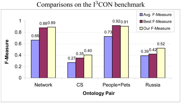
A comparison with the performance of other ontology matching algorithms that participated in the I³CON benchmark evaluations, is shown in Fig. 12. The six participants include the ontology mapping engine, Arctic (Emery & Hart, 2004) from AT&T, LOM (Li, 2004) from Teknowledge, and an alignment algorithm from INRIA, among others. As the shown benchmark evaluations were performed in 2004, many of these alignment algorithms may have since been improved. We show both, the F-measure averaged over the performances of all the participants and the best F-measure obtained for each ontology pair. Note that the best F-measure for each of the ontology pairs was not obtained by the same participant. The ontology pairs of Wine and Weapons have been excluded as benchmark evaluations for these are not available.

Figure 12.

Performance comparison with the other participating ontology matchers. Performance metrics of 6 other ontology matching algorithms are available for the I³CON benchmark. These evaluations were performed in 2004 and some of the participating algorithms may have since been improved.

We observe that the performance of our matching technique, as indicated by the F-measure, is significantly better than the average, and improves on the best performing participant for some of the ontology pairs. Notice that all the participants fare poorly on the tasks of matching CS and Russia ontologies, indicating the difficulty of these tasks. All of our correspondences were obtained within a reasonable amount of time, usually on the order of a few minutes. We used an Intel Xeon 3.6GHz processor and 3GB RAM based machine with Linux. These results demonstrate the comparative benefit of utilizing a lightweight but sophisticated matching algorithm that exploits general-purpose heuristics to guide its search over the space of maps.

In addition to the I³CON benchmark, we also used the Ontology Alignment Evaluation Initiative (OAEI), which utilizes a more systematic approach to evaluate ontology matching algorithms and identify their strengths and weaknesses. OAEI 2006 (Euzenat et al., 2006) provides a series of ontology pairs and associated reference maps, called the benchmark set, each of which is a modification or mutation of a base ontology on bibliographic references (36 concepts, 61 relationships). The benchmark set formulates 3 categories of test ontology pairs: test pairs 101 to 104 pair the base ontology with itself, an irrelevant one, and those expressed in more generalized or specialized languages; test pairs 201–266 compare the base ontology with modifications that include node label mutations, structural mutations, removing edge labels and removing instances; and test pairs 301–304 pair the base ontology with different real-world bibliographic ontologies. In addition to the benchmark set, pairs of real-world ontologies for evaluation are also available. As the true maps for these are not provided, we obtained or computed partial true maps ourselves.

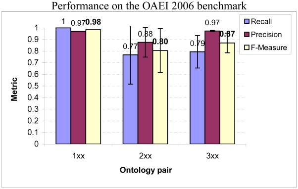
In Fig. 13, we show the performance of our matching algorithm on the benchmark set of OAEI 2006. The perfect recall for the set 1xx indicates that language generalization or specialization did not impact the match performance. Within the set 2xx, our technique compensates for the dissimilarity in node labels by relying on the structural similarities between the ontologies. However, for the ontology pairs where one of the ontologies has randomly generated node labels (for example, pairs 248 to 266), it performs relatively poorly demonstrating its (partial) reliance on the node labels for matching. For many of these pairs, node similarity based on instances proved to be useful. For the pairs where the structure has been altered (for example, pair 221), it utilizes the node label comparisons to reinforce the correspondences. We obtain better performances comparatively when the base bibliographic ontology is compared to different real-world bibliographic ontologies in the set 3xx. While the base ontology focuses exclusively on bibliographic references, the real-world ontologies have wider scopes focusing on peripheral domains, for e.g. departmental organization, as well. Nevetheless, our technique detected the structural and lexical similarities between the ontologies. Notice that the standard deviations for 1xx and 3xx reveal performance variances that are not inordinately large. However, the performance on the set 2xx varies more, in particular, in tests 248 to 266.

Figure 13.

Average recall, precision and F-measure of the identified matches between the ontologies for each category in the OAEI 2006 benchmark tests. The error bars represent the standard deviations of the corresponding metrics for each category.

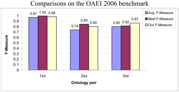
In Fig. 14, we compare the performance of our ontology matching technique with the other best performing algorithms that participated in the benchmark evaluations in 2006. The participants include COMA (Do & Rahm, 2002), FALCON-AO (Hu et al., 2005) and RiMOM (Tang et al., 2006) along with 6 other ontology matching algorithms. Notice that the weakest performances are obtained for the ontology pairs in set 3xx thereby indicating the relative difficulty of the task. Analogous to the I³CON benchmark, no single participating algorithm performed the best in all sets. Our matching technique did not improve on the top performances in the categories 1xx and 2xx, though it exhibited results that were significantly better than the average performance of the best five participating algorithms in each category. For 2xx, its performance would place it second in rank order. It showed better results than all participants for the test set 3xx. In particular, for the test pair 304, over 95% of the concepts and edge labels were correctly matched, though about 65% were correctly matched for the pair 303. This is because the real-world ontology in the latter case had a much wider scope focusing on domains such as departmental organization, than the base ontology.

Figure 14.

Performance comparison with the other participating ontology matchers. Performance metrics of 10 other ontology matching algorithms are available for the OAEI 2006 benchmark. For each category, we identified the five best performing systems (according to their published F-measures) and compared with the average performance among these, and the best performing system. No single participating algorithm performed the best in all sets.

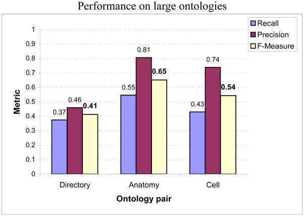
We proceed to evaluate the approach on very large ontology pairs developed independently and often diverse in structure. We utilize three pairs of ontologies in our evaluations: Directory pair consisting of taxonomies that represent Web directories from Google, Yahoo and Looksmart; Anatomy pair consisting of ontologies on the adult mouse anatomy available from Mouse Genome Informatics⁴ and human anatomy from NCI⁵; and the Cell pair (Gennari & Silberfein, 2004) consisting of ontologies on the human cell, developed by FMA (Rosse & Mejino, 2003) and the cell portion of the Gene ontology (GO⁶). The ontologies in the pair differ considerably in the organization of the concepts due to the difference in their development approaches and purposes. Hence, mapping the two facilitates interaction between the communities of anatomists and molecular biologists that each supports, respectively. The Directory and Anatomy taxonomies are the ones that were used in the OAEI 2006 and 2007 contests, respectively. We show the results in Fig. 15. As the true maps for these pairs are not publicly available, we either obtained them by contacting the source (for the Anatomy and Cell pairs) and by inferring them ourselves (for the Directory pair). In order to generate the true correspondences ourselves, we utilized a semi-automated procedure. As the first step, we compared node labels and comments between subsets of partitioned ontologies using our lexical matching technique. We considered both exact and near-exact matches as potential correspondences. Next, we manually filtered out correspondences from this set that did not seem correct. For this, we looked at the labels and comments pertaining to the identified correspondences. Additionally, we identified and visualized their structural contexts in the subsets of the respective ontologies using the Jambalaya tool bundled in Protege (Gennari, Musen, Fergerson, Grosso, Crubezy, Eriksson, Noy, & Tu, 2003). The latter step also resulted in some new correspondences between nodes being added whose node labels did not match. However, as not all true correspondences may have been discovered, the accuracy of our results could be slightly different than shown. The true map for the Anatomy pair contained 1,500 correspondences, the one for the Directory pair contained 1,530 correspondences and the true map for the Cell pair contained 158 hand-crafted correspondences.

Figure 15.

Performances on very large ontology pairs independently developed by different groups of domain experts. The Directory pair includes ontologies consisting of over 2700 and 6600 nodes; Anatomy pair includes those containing over 2800 and 4500 nodes; and the Cell pair consists of ontologies over 1000 and 800 nodes. As ontologies in each pair are independently developed, they additionally exhibit large variations in structure.

Our methodology for matching these large ontology pairs consists of partitioning them using our memory bounded approach as described in Section 9 and executing the GEM on each pair of parts. The parts varied in size and ranged, for example, from 200 nodes to approximately 500 for the Directory pair. Results of evaluating the parts were gathered and aggregated to generate the final results. As fringe nodes are included in the parts, the parts may be evaluated independent of each other. Hence, we could execute several runs in parallel to speed up the computation. Overall, the total evaluation time was approximately 8 hours for the larger ontologies and approximately 2 hours for the Cell pair. The experiments were run using a JDK 1.5 program on a single processor Xeon 3.6GHz, 3GB RAM out of which 1.9GB was utilized by the Java virtual machine, and Linux machines.

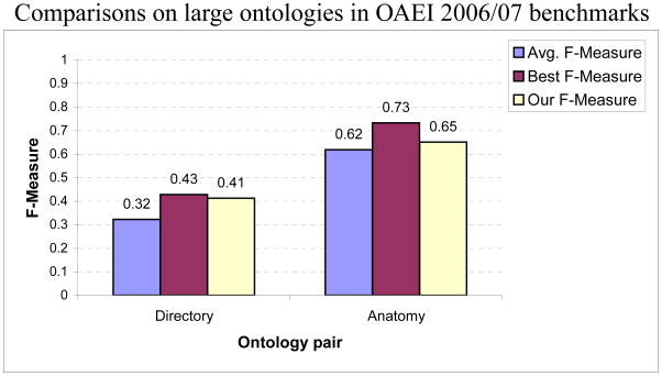
In Fig. 16, we compare our results with those of other alignment tools on the Directory and Anatomy pairs. Note that these comparisons are rough as the true maps used for computing the results may not be identical. For the Directory pair, our approach performed significantly better than the average of the top five performances among the other tools in the OAEI 2006 contest. On the Anatomy pair, our result was significantly better than the average of the performances of the other tools in the OAEI 2007 contest (type C) as well, though lower than the best performance. It would be placed third in rank order for its performance on the Anatomy pair. Interestingly, a majority of the correspondences are between leaf nodes and a naive approach of just comparing node names performs better than the average. The Cell ontology pair is not part of OAEI and alignments by other matchers are not available for comparison.

Figure 16.

Performance comparisons with other ontology matchers on very large ontology pairs. Note that as the number of true correspondences used for computing the results may differ, these results are only roughly comparable. The average F-measure is calculated for the set of the five best performing systems for each ontology pair.

11. Related Work

Previous approaches for matching ontologies have utilized either the instance space associated with the ontologies, the ontology schema structure, or both (see Noy, 2004, for a survey). For example, FCA-Merge (Stumme & Maedche, 2001) and IF-MAP (Kalfoglou & Schorlemmer, 2003) rely on the instances of the concepts and documents annotated by the ontologies to generate the mappings. While FCA-Merge applies linguistic techniques to the instances, IF-MAP utilizes information flow concepts for identifying the map. The GLUE system (Doan et al., 2002), analogous to our approach, utilizes both element-level and structural matchers to identify correspondences between the two ontologies. GLUE uses the instances to compute a similarity measure (Jaccard coefficient) between the concepts, and feeds it to a relaxation labeler that exploits general and domain-specific heuristics to match the ontology schemas. OLA (Euzenat & Valtchev, 2004) views the matching as an optimization problem and utilizes a combination of syntactic matchers for comparing the node labels. OLA formulates a distance metric between the two schemas and iteratively generates a match that optimizes the distance metric. Other approaches that rely heavily on the instance space include BayesOWL (Ding et al., 2005) which uses the instances retrieved off the Web to learn the parameters of the Bayesian network. The joint probability of a pair of concepts, calculated using Jeffrey’s rule for updating distributions using other distributions, is used as a similarity measure. In the same vein, OMEN (Mitra et al., 2004) probabilistically infers a match between classes given a match between parents and children, using Bayesian networks. However, because inference in Bayesian networks, in general, is NP-Hard, OMEN may not scale well to large ontologies. Somewhat analogously, RiMOM (Tang et al., 2006) uses Bayesian decision theory to classify a concept in one ontology as belonging to a class consisting of concept(s) from the other ontology. For this, RiMOM minimizes a log loss function which, similar to our formulation, defines the probability that a concept from one ontology is in correspondence with another given the two ontologies. Both element-level and instance-level matchers are combined to compute the loss function. The FALCON-AO system (Hu et al., 2005) on the other hand proposes metrics for evaluating the structural similarity between the ontology schemas to arrive at a map between the ontologies. The performance of matching approaches that utilize instance spaces is closely linked to the volume of the instances – training data – available. Since many of these methods employ supervised learning, their performance may suffer due to under- or over-fitting caused by insufficient training instances or inexpressive models, respectively. In addition, not all ontologies may be supported by large instance bases. Hence, there is a need for methods that rely on the information in the schema for deriving the map. This helps alleviate the difficulty of obtaining a sizable training set and also exhibited favorable results for many real-world ontology pairs.

Our GEM based algorithm utilizes several features, the label and instance similarities, structural similarities, and an initial seed map to assign the probabilities for the correspondences. We believe that the probability that an entity in the data ontology maps to a model node given a mixture model M depends on all these features. The novelty is in the way that they have been combined resulting in a Bernoulli distribution. This is in addition to a novel EM-based formulation, which distinguishes it from other graph matching approaches such as Falcon-AO and OLA, both of which define a distance metric between ontologies.

As we mentioned before, previous approaches to ontology matching may also be differentiated using the cardinality of the map between the ontologies, that they obtain. Several of the existing approaches such as BayesOWL, GLUE and OMEN (Ding et al., 2005; Doan et al., 2002; Mitra et al., 2004) generate one-one mappings that may be injective between the ontological concepts, with GLUE particularly focusing on taxonomies. These approaches do not allow a node to appear in more than one correspondence between the ontology concepts. Because concepts could be expressed at differing semantic granularities, many-one and many-many maps are relevant. Our approach improves on these by not limiting itself to just one-one maps. Notable exceptions are RiMOM (Tang et al., 2006), which also allows many-one maps and the iMap system (Dhamankar et al., 2004) which generates many-many matches between elements of relational schemas and identifies in some cases how the groups of matched nodes are related. iMap utilizes a host of specialized searchers such as textual, numeric, and date to discover ways in which the schema attributes could be combined and matched. iMap relies heavily on domain knowledge to discover and prune the search space. In contrast, we utilize the node name, instance and structural similarity of ontology schemas to infer the many-one matches. This is in keeping with a secondary aim of our work, which is to gauge how well could approaches that do not utilize external sources or domain knowledge perform the complex mapping tasks.

Of course, no review of the related work is complete without mentioning the vast literature in schema (including entity-relationship diagrams) matching because of our focus on matching ontology schemas and that the schemas considered in these approaches are similar to ontology schemas with constrained relationship types. We refer the reader to Shvaiko and Euzenat (2005) and Doan and Halevy (2005) for recent surveys of the schema matching methods. According to the classification of schema matching methods in, say (Shvaiko & Euzenat, 2005), our approach uses syntactic element-level matchers that are string-based and graph-based structural matchers. Several schema matching systems exist such as COMA (Do & Rahm, 2002) and S-Match (Giunchiglia et al., 2004); we focus on S-Match in some detail here. S-Match aims to generate a semantic match between tree-like schemas by coding the problem of matching as a propositional unsatisfiability problem and utilizing SAT solvers to decide the satisfiability. For selective cases where the propositions may encoded as Horn clauses, the solution is computed in linear time in the number of the sentences. However, S-Match is unwieldy first requiring that the schemas be trees. Though graph-based schemas may be converted into trees efficiently, some knowledge may be lost in the process. Second, S-Match converts node labels into propositional formulas possibly using external sources like WordNet (Miller, 1995). Because of the ambiguity of natural language this may not be a unique conversion, for example, the presence of “and” in a node label could be treated as a disjunction as well as a conjunction between propositions depending on the context. Finally, the presence of disjunctions in the clauses cannot be ruled out and it is unclear how SAT optimization techniques that deal with disjunctions affect the accuracy of the match. However, S-Match exhibited better comparative performance than many of the existing techniques on selected schemas, though evaluations on the benchmark sets are not available. Furthermore, we note that the schema matching techniques are not required to handle labeled relationships.

12. Discussion

We presented a new method for identifying maps between ontologies that model similar domains. We formulated the problem of ontology matching as one of finding the most likely map and solved it iteratively using the GEM technique. Within the GEM approach, we used both, structural similarity between the ontology graphs and lexical similarity between the concept labels and instances to select the map. Similar to some of the recent approaches, we generate inexact matches between the ontologies that may result in multiple nodes of one ontology to be mapped to a single node of the other; such methods have a wider applicability.

While our initial experimental results illustrated the good performance of our method, they also highlighted its inability to scale to large ontologies. To address this limitation, we modified the GEM to operate on smaller subsets within partitions of the ontologies. Our empirical results on benchmarks such as I³CON and OAEI 2006 indicate the favorable performance of the method and provide support for lightweight but sophisticated approaches to matching ontologies.

The systematic evaluation using the test ontology pairs provided by OAEI revealed some of the strengths and weaknesses of our method. First, because we utilize the lexical similarity in concept labels to partly establish the likelihood of a map, our technique exhibits a weak performance where the node labels are highly dissimilar. We offset this limitation by utilizing instances, if available. Examples of affected tasks include matching ontologies on similar domains written in different languages and ontologies expressed using alternate standards. However, the performance improves if the structures of the ontologies are comparable. Second, small changes in the structures such as flattening or expansion of the concept hierarchy did not significantly impact the performance. This is because the most likely map that we discover often turns out to be the correct one too, thereby reducing the impact of such structural changes. Of course, the task of matching ontologies that are both syntactically and structurally disparate is the most difficult, for example, matching ontologies written in different languages with partially overlapping scopes.

We note that further efficiency is needed for performing the optimization step. This is especially pertinent, if we allow both many-one and many-many maps between the ontologies. In this regard, we intend to combine heuristics with Markov Chain Monte Carlo methods (Gilks, Richardson, & Spiegelhalter, 1995) to focus the search in the model space. We are also investigating the efficacy of utilizing sources of general background knowledge and different ways in which structural contexts may be used efficiently to discover a map.

References

- Berners-Lee T. Notation 3: An rdf language for the semantic web. Tech. rep. World Wide Web Consortium (W3C) 2000 [Google Scholar]
- Brickley D, Guha R. World Wide Web Consortium (W3C) 2004. RDF Vocabulary Description Language 1.0: RDF Schema. Tech. rep., Recommendation. [Google Scholar]
- Cohen WW, Ravikumar P, Fienberg SE. A comparison of string distance metrics for name-matching tasks. Workshop on Information Integration on the Web, International Joint Conference on Artificial Intelligence (IJCAI).2003. [Google Scholar]
- Cross A, Hancock E. Graph matching with a dual-step em algorithm. IEEE Transactions on Pattern Analysis and Machine Intelligence. 1998;20(11):1236–1253. [Google Scholar]
- Titterington DM, Smith AFM, UEM . Statistical analysis of finite mixture distributions. Wiley; New York: 1985. [Google Scholar]
- Dempster AP, Laird NM, Rubin DB. Maximum likelihood from incomplete data via the em algorithm. Journal of the Royal Statistical Society, Series B (Methodological) 1977;39:1–38. [Google Scholar]
- Dhamankar R, Lee Y, Doan A, Halevy A, Domingos P. imap: Discovering complex semantic matches between database schemas. ACM Conference on Management of Data (SIGMOD); 2004. pp. 383–394. [Google Scholar]
- Ding Z, Peng Y, Pan R, Yu Y. A Bayesian Methodology towards Automatic Ontology Mapping. Workshop on Context & Ontologies, Twentieth Conference on Artificial Intelligence (AAAI).2005. [Google Scholar]
- Do HH, Rahm E. Coma - a system for flexible combination of schema matching approaches. International Conference on Very Large Databases (VLDB); 2002. pp. 610–621. [Google Scholar]
- Doan A, Halevy A. Semantic integration research in the database community. a brief survey. AI Magazine. 2005;26(1):83–94. [Google Scholar]
- Doan A, Madhavan J, Domingos P, Halevy A. World Wide Web. ACM Press; 2002. Learning to map between ontologies on the semantic web; pp. 662–673. [Google Scholar]
- Emery P, Hart L. Artic: Ontology mapping engine. Tech. rep., CODIP Project. 2004 http://codip.grci.com/, AT&T Government Solutions.
- Euzenat J, Mochol M, Shvaiko P, Stuckenschmidt H, Svab O, Svatek V, Rage W, Yatskevich M. Results of the ontology alignment 2006 inititiative. International Workshop on Ontology Matching, International Semantic Web Conference (ISWC).2006. [Google Scholar]
- Euzenat J, Shvaiko P. Ontology Matching. Springer; 2007. [Google Scholar]
- Euzenat J, Valtchev P. Similarity-based ontology alignment for owl-lite. European Conference on Artificial Intelligence (ECAI); 2004. pp. 333–337. [Google Scholar]
- Gennari J, Musen MA, Fergerson RW, Grosso WE, Crubezy M, Eriksson H, Noy NF, Tu SW. The evolution of protégé: An environment for knowledge-based systems development. International Journal of Human-Computer Studies. 2003;58(1):89–123. [Google Scholar]
- Gennari JH, Silberfein A. Leveraging an alignment between two large ontologies: Fma and go. Seventh International Protege Conference.2004. [Google Scholar]
- Gilks WR, Richardson S, Spiegelhalter D. Markov Chain Monte Carlo in Practice. Chapman and Hall; CRC: 1995. [Google Scholar]
- Giunchiglia F, Shvaiko P, Yatskevich M. S-match: An algorithm and an implementation of semantic matching; European Semantic Web Symposium; 2004. pp. 61–75. [Google Scholar]
- Hayes J, Gutierrez C. Bipartite graphs as intermediate models for rdf graphs. International Semantic Web Conference (ISWC); 2004. pp. 47–61. [Google Scholar]
- Hu W, Jian N, Qu Y, Wang Y. GMO: A graph matching for ontologies. Workshop on Integrating Ontologies, Conference on Knowledge Capture (K-CAP).2005. [Google Scholar]
- Hughes T, Ashpole B. Information interpretation and integration conference. 2004 http://www.atl.lmco.com/projects/ontology/i3con.html.
- Kalfoglou Y, Schorlemmer M. If-map: an ontology mapping method based on information flow theory. Journal on Data Semantics. 2003;1(1):98–127. [Google Scholar]
- Lauritzen S. The em algorithm for graphical association models with missing data. Computational Statistics and Data Analysis. 1995;19:191–201. [Google Scholar]
- Lee Y, Sayyadian M, Doan A, Rosenthal A. etuner: Tuning schema matching software using synthetic scenarios. Very Large Databases Journal. 2007;16(1) [Google Scholar]
- Li J. Lom: A lexicon-based ontology mapping tool. Workshop on Performance Metrics for Intelligent Systems (PerMIS), Information Interpretation and Integration Conference.2004. [Google Scholar]
- Luo B, Hancock E. Structural graph matching using the em algorithm and singular value decomposition. Graph Algorithms and Computer Vision. 2001;23(10):1120–1136. [Google Scholar]
- Manola F, Miller E. Rdf primer. Tech. rep., Recommendation. World Wide Web Consortium (W3C) 2004 [Google Scholar]
- McGuinness D, Harmelen FV. Owl web ontology language overview. Tech. rep., Recommendation. World Wide Web Consortium (W3C) 2004 [Google Scholar]
- McLachlan G, Krishnan T. The EM Algorithm and its Extensions. Wiley; New York: 1995. [Google Scholar]
- Miller AG. Wordnet: A lexical database for english. Communications of the ACM. 1995;38(11):39–41. [Google Scholar]
- Milo T, Zohar S. Using schema matching to simplify heterogenous data translation. International Conference on Very Large Databases (VLDB); 1998. pp. 122–133. [Google Scholar]
- Mitra P, Noy N, Jaiswal A. OMEN: A probabilistic ontology mapping tool. Workshop on Meaning, Coordination and Negotation, International Semantic Web Conference (ISWC).2004. [Google Scholar]
- Noy NF. Semantic integration: A survey of ontology-based approaches. SIGMOD Record. 2004;33:65–70. [Google Scholar]
- Qu Y, Hu W, Cheng G. Constructing virtual documents for ontology matching. Fifteenth International Conference on World Wide Web; 2006. pp. 23–31. [Google Scholar]
- Rosse C, Mejino J. A reference ontology for biomedical informatics: the foundational model of anatomy. Journal of Biomedical Informatics. 2003;36:478–500. doi: 10.1016/j.jbi.2003.11.007. [DOI] [PubMed] [Google Scholar]
- Shvaiko P, Euzenat J. A survey of schema-based matching approaches. Journal of Data Semantics. 2005;4:146–171. [Google Scholar]
- Smith TF, Waterman MS. Identification of common molecular subsequences. Journal of Molecular Biology. 1981;147:195–197. doi: 10.1016/0022-2836(81)90087-5. [DOI] [PubMed] [Google Scholar]
- Stuckenschmidt H, Klein M. Structure based partitioning of large concept hierarchies. International Semantic Web Conference (ISWC); 2004. pp. 289–303. [Google Scholar]
- Stumme G, Maedche A. FCA-MERGE: Bottom-up merging of ontologies. International Joint Conference on Artificial Intelligence (IJCAI); 2001. pp. 225–234. [Google Scholar]
- Tang J, Li J, Liang B, Huang X, Li Y, Wang K. Using bayesian decision for ontology mapping. Journal of Web Semantics. 2006;4(4):243–262. [Google Scholar]