Characterizing fiber directional uncertainty in diffusion tensor MRI

Abstract

Image noise in diffusion tensor MRI (DT-MRI) causes errors in the measured tensor, and hence variance in the estimated fiber orientation. Uncertainty in fiber orientation has been described using a circular “cone of uncertainty” (CU) around the principal eigenvector of the diffusion tensor. The cone of uncertainty has proved to be a useful construct for quantifying and visualizing the variability of DT-MRI parameters and fiber tractography. The assumption of circularity of the CU has not been tested directly, however. In this work, bootstrap analysis and simple theoretical arguments were used to show that the cone of uncertainty is elliptical and multivariate normal in the vast majority of white matter voxels for typical measurement conditions. The dependence of the cone angle on signal-to-noise ratio and eigenvalue contrast was established. The major and minor cone axes are shown to be coincident with the second and third eigenvectors of the tensor, respectively, in the limit of many uniformly spaced diffusion encoding directions. The deviation between the major cone axis and the second eigenvector was quantified for typical sets of diffusion weighting directions. The elliptical cone of uncertainty provides more realistic error information for fiber tracking algorithms and a quantitative basis for selecting diffusion tensor imaging acquisition protocols.

INTRODUCTION

Diffusion tensor MRI (DT-MRI) provides information on water molecular diffusion based on a series of images with diffusion weighting applied in at least six non-collinear directions (1,2). Given the effective diffusion tensor, it is possible to characterize tissue microstructure using the directional dependence of diffusion in vivo (3,4). In addition, this directional information has been exploited to estimate the paths of fiber bundles in the brain in order to infer axonal connectivity (5). In this case, the principal eigenvector (i.e., the estimated direction of maximum diffusivity), v₁, is taken to be parallel to the local fiber bundle. In the presence of image noise, however, perturbations of the diffusion tensor field introduce errors in the estimated diffusion anisotropy (6-8) and fiber direction (9,10).

The directional uncertainty in v₁ has been characterized by the ‘cone of uncertainty’ (11,12). This was defined as a circular cone with axis along the expectation value of v₁ and cone angle equal to the uncertainty (i.e., confidence interval) in the orientation of v₁ . The cone of uncertainty (CU) is particularly useful for visualizing the uncertainty in fiber orientation and predicting error in MR fiber tractography. However, Lazar and Alexander (13,14) showed that errors in MR tractography typically have an elliptical distribution, and noted that an elliptical CU is expected in voxels that lack axially symmetric diffusion. They measured the dispersion of fiber tracking errors in a plane perpendicular to the fiber axis at some distance from the seed points. They noted a strong correlation between the direction of the greatest dispersion of tracking errors and the second eigenvector of the tensor (corresponding to the second largest diffusivity). The same relationship existed between the direction of the smallest dispersion of tracking errors and the third eigenvector of the tensor (corresponding to the smallest diffusivity). In this paper, we provide a general explanation for this observation, and present results of experimental and theoretical studies of the properties of the CU. In particular, we tested the symmetry and multivariate normality of principal eigenvector errors, and characterized the dependence of the associated CU on image noise, diffusion anisotropy and eigenvalue contrast. In addition, we investigated the coincidence between the tensor eigenvectors and the axes of the elliptical cone, and how this correspondence depends on the diffusion gradient encoding scheme. Some of this work has appeared previously in abstract form (15). Koay et al have recently proposed a similar construction of the elliptical cone of uncertainty (16).

THEORY

The dependence of the major eigenvector (i.e., the eigenvector corresponding to the largest eigenvalue), v₁ , on tensor errors can be found from first order perturbation theory (10,11,17) or simple error analysis (18). The major eigenvector of the diffusion tensor satisfies the eigenvalue equation

$$\mathbf{D}{\mathbf{v}}_1={\lambda }_1{\mathbf{v}}_1,$$ [1]

where D and λ₁ are the true tensor and major eigenvalue (i.e., λ₁ > λ₂ ≥ λ₃), respectively. Taking the differential of both sides of Eq. [1] gives a relation among the errors in these quantities:

$$\delta \mathbf{D}\cdot {\mathbf{v}}_1+\mathbf{D}\cdot \delta {\mathbf{v}}_1=\delta {\lambda }_1\cdot {\mathbf{v}}_1+{\lambda }_1\cdot \delta {\mathbf{v}}_1.$$ [2]

The tensor is represented by a 3 × 3 symmetric matrix and the principal eigenvector is a 3 × 1 column vector. Multiplying Eq. [2] by the transpose of the middle eigenvector v₂ , denoted by ${\mathbf{v}}_2^{\mathrm{T}}$, yields

$${\mathbf{v}}_2^{\mathrm{T}}\cdot \delta \mathbf{D}\cdot {\mathbf{v}}_1+{\mathbf{v}}_2^{\mathrm{T}}\mathbf{D}\cdot \delta {\mathbf{v}}_1=\delta {\lambda }_1\cdot {\mathbf{v}}_2^{\mathrm{T}}{\mathbf{v}}_1+{\lambda }_1{\mathbf{v}}_2^{\mathrm{T}}\cdot \delta {\mathbf{v}}_1.$$ [3]

Since the eigenvectors are orthogonal,

$${\mathbf{v}}_2^{\mathrm{T}}{\mathbf{v}}_1=0.$$ [4]

The eigenvalue equation for v₂ is

$$\mathbf{D}{\mathbf{v}}_2={\lambda }_2{\mathbf{v}}_2,$$

and the transpose of this relation is

$${\mathbf{v}}_2^{\mathrm{T}}\mathbf{D}={\lambda }_2{\mathbf{v}}_2^{\mathrm{T}},$$

Since D is symmetric. Multiplying on the right by δv₁, the error in v₁, gives

$${\mathbf{v}}_2^{\mathrm{T}}\mathbf{D}\cdot \delta {\mathbf{v}}_1={\lambda }_2{\mathbf{v}}_2^{\mathrm{T}}\cdot \delta {\mathbf{v}}_1.$$ [5]

Substituting Eqs. [4,5] into Eq. [3] gives

$${\mathbf{v}}_2^{\mathrm{T}}\cdot \delta \mathbf{D}\cdot {\mathbf{v}}_1+{\lambda }_2{\mathbf{v}}_2^{\mathrm{T}}\cdot \delta {\mathbf{v}}_1={\lambda }_1{\mathbf{v}}_2^{\mathrm{T}}\cdot \delta {\mathbf{v}}_1.$$

The component of the v₁ error (δ v₁) in the v₂ direction is therefore

$${\mathbf{v}}_2^{\mathrm{T}}\cdot \delta {\mathbf{v}}_1=\frac{{\mathbf{v}}_2^{\mathrm{T}}\cdot \delta \mathbf{D}\cdot {\mathbf{v}}_1}{{\lambda }_1-{\lambda }_2}.$$ [6]

Replacing v₂ by v₃ in Eq. [3] leads to an analogous expression for the component of the v₁ error in the v₃ direction:

$${\mathbf{v}}_3^{\mathrm{T}}\cdot \delta {\mathbf{v}}_1=\frac{{\mathbf{v}}_3^{\mathrm{T}}\cdot \delta \mathbf{D}\cdot {\mathbf{v}}_1}{{\lambda }_1-{\lambda }_3}.$$ [7]

The eigenvectors have unit length, so for example,

$${\mathbf{v}}_1^{\mathrm{T}}\cdot {\mathbf{v}}_1=1.$$

Differentiating both sides of this equation yields

$$\delta {\mathbf{v}}_1^{\mathrm{T}}\cdot {\mathbf{v}}_1+{\mathbf{v}}_1^{\mathrm{T}}\cdot \delta {\mathbf{v}}_1=0.$$

Since the two terms on the left are scalars and each is the transpose of the other, they must be equal. Hence,

$${\mathbf{v}}_1^{\mathrm{T}}\cdot \delta {\mathbf{v}}_1=0,$$ [8]

The v₁ error, δ v₁, is perpendicular to the v₁ direction. Taken together, Eqs. [6-8] specify the three orthogonal components of the error in the major eigenvector corresponding to a given tensor error, δ D .

The covariance matrix, Σ_v1 , for v₁ in the {v₂, v₃} plane gives the variance of δ v₁ along v₂ and v₃ on the diagonal and the covariance of these components in the off-diagonal elements:

$$\begin{array}{cc}\hfill {\Sigma }_{{\mathbf{v}}_1}=& \left[\begin{array}{cc}\hfill \langle {\left({\mathbf{v}}_2^{\mathrm{T}}\cdot \delta {\mathbf{v}}_1\right)}^2\rangle \hfill & \hfill \langle \left({\mathbf{v}}_2^{\mathrm{T}}\cdot \delta {\mathbf{v}}_1\right)\cdot \left({\mathbf{v}}_3^{\mathrm{T}}\cdot \delta {\mathbf{v}}_1\right)\rangle \hfill \\ \hfill \langle \left({\mathbf{v}}_2^{\mathrm{T}}\cdot \delta {\mathbf{v}}_1\right)\cdot \left({\mathbf{v}}_3^{\mathbf{T}}\cdot \delta {\mathbf{v}}_1\right)\rangle \hfill & \hfill \langle {\left({\mathbf{v}}_3^{\mathrm{T}}\cdot \delta {\mathbf{v}}_1\right)}^2\rangle \hfill \end{array}\right]\hfill \\ \hfill =& \left[\begin{array}{cc}\hfill \frac{\langle {\left({\mathbf{v}}_2^{\mathrm{T}}\cdot \delta \mathbf{D}\cdot {\mathbf{v}}_1\right)}^2\rangle }{{({\lambda }_1-{\lambda }_2)}^2}\hfill & \hfill \frac{\langle \left({\mathbf{v}}_2^{\mathrm{T}}\cdot \delta \mathbf{D}\cdot {\mathbf{v}}_1\right)\left({\mathbf{v}}_3^{\mathrm{T}}\cdot \delta \mathbf{D}\cdot {\mathbf{v}}_1\right)\rangle }{({\lambda }_1-{\lambda }_2)({\lambda }_1-{\lambda }_3)}\hfill \\ \hfill \frac{\langle \left({\mathbf{v}}_2^{\mathrm{T}}\cdot \delta \mathbf{D}\cdot {\mathbf{v}}_1\right)\left({\mathbf{v}}_3^{\mathrm{T}}\cdot \delta \mathbf{D}\cdot {\mathbf{v}}_1\right)\rangle }{({\lambda }_1-{\lambda }_2)({\lambda }_1-{\lambda }_3)}\hfill & \hfill \frac{\langle {\left({\mathbf{v}}_3^{\mathrm{T}}\cdot \delta \mathbf{D}\cdot {\mathbf{v}}_1\right)}^2\rangle }{{({\lambda }_1-{\lambda }_3)}^2}\hfill \end{array}\right],\hfill \end{array}$$ [9]

using Eqs. [6,7]. Diagonalizing the covariance matrix identifies the principal components of v₁ variation. To be explicit, suppose the z axis is chosen to be parallel to v₁ . For convenience we choose the x and y axes to be parallel to v₂ and v₃ , respectively. Because of measurement errors in D, the estimated principal eigenvector will have components in the x and y directions. Let the coordinates of δ v₁ be (x, y). In this case, Eq. [9] can be written as

$$\begin{array}{cc}\hfill {\Sigma }_{{\mathbf{v}}_1}=& \left[\begin{array}{cc}\hfill \langle x^2\rangle \hfill & \hfill \langle x\cdot y\rangle \hfill \\ \hfill \langle x\cdot y\rangle \hfill & \hfill \langle y^2\rangle \hfill \end{array}\right]\hfill \\ \hfill =& \left[\begin{array}{cc}\hfill \frac{\langle \delta D_{xz}^2\rangle }{{({\lambda }_z-{\lambda }_x)}^2}\hfill & \hfill \frac{\langle \delta D_{xz}\cdot \delta D_{yz}\rangle }{({\lambda }_z-{\lambda }_x)({\lambda }_z-{\lambda }_y)}\hfill \\ \hfill \frac{\langle \delta D_{xz}\cdot \delta D_{yz}\rangle }{({\lambda }_z-{\lambda }_x)({\lambda }_z-{\lambda }_y)}\hfill & \hfill \frac{\langle \delta D_{yz}^2\rangle }{{({\lambda }_z-{\lambda }_y)}^2}\hfill \end{array}\right],\hfill \end{array}$$ [10]

where $\delta D_{xy}\equiv {\mathbf{e}}_x^{\mathrm{T}}\cdot \delta \mathbf{D}\cdot {\mathbf{e}}_y$, $\delta D_{xz}\equiv {\mathbf{e}}_x^{\mathrm{T}}\cdot \delta \mathbf{D}\cdot {\mathbf{e}}_z$, $\delta D_{yz}\equiv {\mathbf{e}}_y^{\mathrm{T}}\cdot \delta \mathbf{D}\cdot {\mathbf{e}}_z$ and e_x, e_y, and e_z are unit vectors along the coordinate axes. If the errors δ v₁ have a multivariate normal distribution then they can be characterized concisely using the eigenvalues σ₁ and σ₂ (σ₁ ≥ σ₂) and corresponding eigenvectors e₁ and e₂ of the covariance matrix. In this case, the probability density function for δ v₁ is

$$P\left(\delta {\mathbf{v}}_1\right)=\frac{1}{2\pi {\mid {\Sigma }_{{\mathbf{v}}_1}\mid }^{1∕2}}\cdot \exp \left(-\frac{1}{2}\delta {\mathbf{v}}_1^{\mathrm{T}}\cdot {\Sigma }_{{\mathbf{v}}_1}^{-1}\cdot \delta {\mathbf{v}}_1\right),$$ [11]

assuming the mean value of δv₁ is zero. A contour of constant probability density is defined by the set of coordinates (x, y) that satisfy the relation

$$\left[xy\right]\cdot {\Sigma }_{{\mathbf{v}}_1}^{-1}\cdot \left[\begin{array}{c}\hfill x\hfill \\ \hfill y\hfill \end{array}\right]=c^2$$ [12]

with constant c. The solution to this equation is an ellipse with semi-major axis of length $c\sqrt{{\sigma }_1}$ parallel to e₁ and semi-minor axis of length $c\sqrt{{\sigma }_2}$ parallel to e₂ (19). If the eigenvalues of the covariance matrix are not equal, then the errors are not circularly symmetric in the (x, y) plane. In the general multivariate normal case, the errors have an ellipsoidal distribution, the major and minor axes of the ellipse given by the eigenvectors of the covariance matrix. In the limit of many uniformly distributed diffusion measurement directions, the off-diagonal terms go to zero, $\langle \delta D_{xz}\cdot \delta D_{yz}\rangle =0$, so Σ_v1 is diagonal in the eigenframe of the tensor (see Appendix). Further, it is shown that if λ₂>λ₃ then $\langle \delta D_{xz}^2\rangle >\langle \delta D_{yz}^2\rangle$. This implies that the upper-left element in Eq. [10] is the largest eigenvalue of Σ_v1 , and hence the major axis of the ellipsoidal distribution is parallel to v₂. To test whether this relation holds for practical (i.e., finite) diffusion encoding schemes, we performed the experiments described below. Before leaving this topic, however, we should note that if the tensor eigenvalues are equal (λ₁ = λ₂ or λ₁ = λ₂ = λ₃ ), then Eqs. [6,7] fail. In this case, degenerate perturbation theory must be used to evaluate the δ v₁ errors (10). However, the exactly degenerate situation is unlikely to arise in routine white matter tractography.

METHODS

DT-MRI acquisition

The study protocol was approved by Vanderbilt University’s institutional review board. Diffusion weighted images were acquired in a healthy adult using a 3 Tesla whole body GE scanner (40 mT/m maximum gradient strength, 150 mT/m/ms maximum slew rate). A dual spin echo EPI pulse sequence was used to acquire images with diffusion weighting (1000 s/mm²), applied in six non-collinear directions (20), as well as a set of images with no diffusion weighting. All images (7 images in each of 30 slice locations) had an 89 ms echo time, 9 s repetition time, 128×128 acquisition reconstructed to a 256×256 image matrix, and 2×2×4 mm³ voxel size. A total of 37 identical scans were acquired in one imaging session. Image alignment was assessed by visual inspection of the difference between the first and the last images of each slice during the session (this revealed no significant differences in head position). All of the image data were averaged in order to estimate the ‘true’ diffusion tensor, and ‘true’ orientation of the principal eigenvector, v₁, in each voxel with high precision. Smaller sets of the image data were also averaged to investigate the dependence of v₁ errors on net image SNR.

Generation of principal components and CU

Bootstrap resampling (21) was used to select N_A acquisitions to average (N_A ≤ 37). Each set of N_A acquisitions is one sample. We formed 100, 200, 500 and 1000 samples with replacement, then calculated the diffusion tensor and major eigenvector for each sample in each voxel. The eigenvalue-eigenvector pairs were sorted according to their similarity with the estimated ‘true’ values using a tensor overlap measure (9). Each estimate, ${\widehat{\mathbf{v}}}_1$, of the major eigenvector was projected onto the plane perpendicular to the ‘true’ v₁ (i.e., the plane defined by the best estimates of the two other eigenvectors, v₂ and v₃):

$${\mathrm{Proj}}_{{\mathbf{v}}_j}\left({\widehat{\mathbf{v}}}_1\right)=\left({\mathbf{v}}_j^{\mathrm{T}}{\widehat{\mathbf{v}}}_1\right){\mathbf{v}}_j,j=2,3.$$ [13]

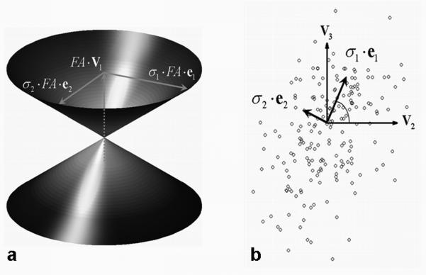
A principal component (PC) analysis was used to analyze the distribution of ${\widehat{\mathbf{v}}}_1$ projections on the {v₂, v₃} plane and hence determine the major and minor axes of the CU. The covariance matrix of projection coordinates was diagonalized. The eigenvalues, σ₁ and σ₂ , and corresponding (normalized) eigenvectors, e₁ and e₂ , of the covariance matrix were used to construct an ellipse parallel to the {v₂, v₃} plane and centered on v₁ :

$$\stackrel{\rightharpoonup }{\mathbf{r}}\left(\phi \right)={\mathbf{v}}_1+{\sigma }_1\cos \phi {\mathbf{e}}_1+{\sigma }_2\sin \phi {\mathbf{e}}_2\phi \in [0,2\pi ].$$ [14]

The eigenvectors, e₁ and e₂ , define the major and minor axes of the ellipse. The CU was then defined as the set of line segments from the origin to the ellipse, which is the directrix of the conical surface (Eq. [14]). For display purposes, all dimensions were scaled by the tensor’s fractional anisotropy (FA) (3) (see Fig. 1a).

Figure 1.

Construction of the cone of uncertainty (a) based on the projection of ${\widehat{\mathbf{v}}}_1$ (circles) onto the {v₂, v₃} plane (b) for a representative white matter voxel with 6 scans averaged (FA = 0.73, 200 bootstrap samples). The size of the cone (i.e., its height and major and minor axes) is scaled by FA, and the directions of the major and minor cone axes (denoted by e₁ and e₂ , respectively) are given by the principal components (σ₁ ·e₁ and σ₂ ·e₂) of the v₁ error distribution shown as circles in (b). The coincidence angle (↼) between e₁ and v₂ is also shown (b).

Symmetry, normality and cone angles of the CU

The equality of the major and minor axes of the ellipse (i.e., the standard deviations of the PCs’) was tested using the method by Bartlett (22). The multivariate normality of the distribution of ${\widehat{\mathbf{v}}}_1$ projections was tested using the method of Mardia (23,24) for multivariate skewness and kurtosis and mapped for 200 bootstrap samples with two levels of image SNR (i.e., N_A). We define the cone angles as θ_i ≡ tan^-1 (σ_i) , i = 1,2 . In the limit of many uniformly distributed gradients, the cone angle can be approximated using Eq. [9] as

$${\theta }_i\approx \frac{{\left[\langle {\left({\mathbf{v}}_{i+1}^{\mathrm{T}}\cdot \delta \mathbf{D}\cdot {\mathbf{v}}_1\right)}^2\rangle \right]}^{1∕2}}{{\lambda }_1-{\lambda }_{i+1}},i=1,2.$$ [15]

Bootstrap estimates of the cone angles were compared to this expression to verify the simple theoretical model of fiber directional uncertainty. The cone angles were also compared in voxels with different levels of FA and image SNR.

Coincidence between the CU and tensor principal axes

To quantify the alignment of the major cone axis with the tensor eigenvectors, we defined the coincidence angle to be the angle between e₁ and v₂ (see Fig 1b). Because we used the same 6 direction gradient vector set (20) during the entire experiment, simulations were used to study how the coincidence angle depends on the choice of gradient vector set. Several gradient sets were used, these were labeled ‘original #’ (# is the number of gradient vectors) and included ‘original 6′ (20), ‘original 12′ (25), ‘original 21′ (second order icosahedral tessellation of the unit sphere), ‘original 92′ (46 directions, given by third order icosahedral tessellation, and their opposites). The ‘original #’ scheme is the set of gradient vectors originally described in the corresponding references or determined numerically (26). The ‘rotated #’ scheme is labeled similarly, e.g., ‘rotated 6′, after 45 degrees rotation of the ‘original’ scheme around the Z axis in the gradient coordinate system. For the simulation, we used the measured noise standard deviation and ‘true’ diffusion tensor (obtained by averaging the entire data set) to generate diffusion weighted and non-weighted signals, including simulated random noise, for each gradient vector scheme listed above. This simulation was repeated 200 times, and the simulated data were then analyzed to determine the coincidence angle between the major axis of the CU and the second eigenvector of the ‘true’ tensor. Hence, for this part of the study, the axes of the CU were estimated via Monte Carlo simulation for each gradient vector set.

The dependence of the coincidence angle on the choice of gradient vector scheme can be understood in terms of the ${\widehat{\mathbf{v}}}_1$ covariance matrix elements, Eq. [9], in the tensor eigenvector frame. We selected a representative voxel in the splenium of corpus callosum and simulated diffusion weighted signals (as described above) in the tensor eigenframe based on the gradient schemes listed above. In the simulation, we used the coordinate naming convention of the Appendix: $\widehat{x}\Vert {\widehat{\mathbf{v}}}_2$, $\widehat{y}\Vert {\widehat{\mathbf{v}}}_3$, and $\widehat{z}\Vert {\widehat{\mathbf{v}}}_1$ and simulated the effect of noise using Monte Carlo simulations. In each trial, the errors δ D_ij of the diffusion tensor elements were calculated. The covariance matrix elements of Eq. [9] were then plotted to show the dependence of the matrix elements on the choice of gradient scheme.

RESULTS

Comparison of bootstrap and theoretical results

Bootstrap estimates of the projection of ${\widehat{\mathbf{v}}}_1$ onto the {v₂, v₃} plane (i.e., the v₁ error) are shown schematically for a representative white matter voxel in the splenium of the corpus callosum in Fig. 1b. The principal components of the distribution are also shown. The principal components of v₁ errors can be estimated from this distribution or from Eq. [9]. These two estimates were compared in order to test the accuracy of the simple theoretical model applied to in vivo data. The standard deviation of v₁ errors for the minor principal component calculated using perturbation theory (σ_PT , the square root of the smaller eigenvalue of the covariance matrix in Eq. [9]) was correlated with the bootstrap estimate (σ_BS ) for the voxels whose linearity index (27) C_l > 0.3, to exclude voxels with nearly isotropic diffusion, for example in the CSF (N_A = 6 and 200 bootstrap samples were used). The correlation was excellent (R² = 0.998 and slope = 0.99 with offset ≈ 0). Results were similar for the major principal component (R² = 0.994 and slope = 0.98 with offset ≈ 0). The agreement between the two estimates of v₁ errors is excellent (for C_l > 0.3), with the R² and slope of the fit nearly equal to one.

Test for symmetry and multivariate normality of CU

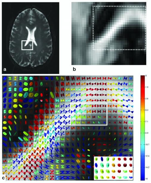
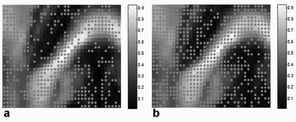
The directional uncertainty in ${\widehat{\mathbf{v}}}_1$ is represented by the cone of uncertainty centered on v₁ as shown in Fig. 2. The CUs for voxels in the outlined region of Figs. 2a and b are shown in Fig. 2c for N_A = 6 and 200 bootstrap samples. The CUs for voxels in the outlined region of Fig. 2c are redrawn (inset in the lower right corner) as viewed along the local v₁ axis to show the cones’ eccentricity clearly. Each cone is color coded according to base 10 logarithm of the p-value from the test of the circular symmetry of ${\widehat{\mathbf{v}}}_1$ errors in the {v₂, v₃} plane (i.e., the test of equality of the principal component variances). Hence, color indicates the statistical significance of CU eccentricity. As the color varies from red to blue, the cones of uncertainty change from nearly circular (for p > 0.05, log₁₀(p) = log₁₀(0.05) > -1.3) to highly eccentric. Most of the voxels in the ROI exhibit non-circular CUs (Table 1) based on bootstrap comparisons of major and minor cone axes. In the second analysis, every voxel in the ROI was tested for multivariate normality of ${\widehat{\mathbf{v}}}_1$ errors using the test of multivariate skewness and kurtosis (23,24). Figure 3 shows that most white matter voxels exhibit multivariate normality of the error distribution based on this test. According to the circular symmetry test, the estimated fraction of cones with significant eccentricity increases as the number of bootstrap samples and N_A increase (Table 1) and the fraction of voxels with normally distributed error increases with increasing N_A (Figure 3).

Figure 2.

A T₂-weighted image (a) showing an ROI and its FA map (b). The white dotted area in (b) is used in (c) for CU visualization. The CUs (using 6 averages, 200 bootstrap samples) are color coded according to base 10 logarithm of the p-value from the test for zero eccentricity. Low probability of circularity (zero eccentricity) is shown as dark blue, while high probability is shown as red (c). The base of each cone in the square region in (c) is shown in the local v₂ (horizontal in the inset) - v₃ (vertical) plane at the lower right corner in (c). Those cones are uniformly scaled for clear visualization.

Table 1.

Percentage of voxels in the ROI (Fig. 2a) with eccentric cones of uncertainty (p-value ≤ 0.05) from bootstrap results.

Number of acquisitions averaged	Number of bootstrap samples
	100	200	500	1000
2	67.9	81.1	90.5	94.8
4	76.0	84.8	93.6	96.2
6	77.4	86.3	93.6	96.3
12	79.1	88.0	95.0	97.0
24	81.5	88.4	94.4	97.3

Figure 3.

Mapped results of the test of multivariate normality (skewness and kurtosis) for the ROI (Fig. 2a) superimposed on the FA map. Dots indicate multivariate normality in fiber directional error with 4 (a) and 12 (b) averaged scans and 200 bootstrap samples for p-value of 0.05. The fractional number of voxels with multivariate normal error over the whole ROI is approximately 47 % (a) and 64 % (b), and increases as N_A increases.

Characterization of fiber directional uncertainty as a cone angle

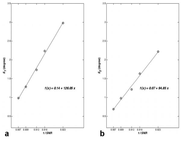
The cone angle, θ , was defined for both the major and minor axes of the cone base (θ₁ and θ₂ , respectively). The cone angle is the arc tangent of the standard deviation of the ${\widehat{\mathbf{v}}}_1$ error in the corresponding principal component direction (see Fig. 1a). The dependence of the cone angle on image SNR is shown for a representative voxel in the splenium of the corpus callosum in Fig. 4. Here the cone angle is plotted as a function of 1/SNR, where SNR = N_A^1/2 ·SNR₀, and SNR₀ is measured on a single non-weighted image (SNR₀ = 31.3). As expected, the cone angle is proportional to the standard deviation of image noise (i.e., to SNR^-1). All voxels tested showed similar dependence on SNR (data not shown).

Figure 4.

Cone angle of the major (θ₁) and minor (θ₂) axes fit to a linear function of SNR^-1 ($\mathrm{SNR}=N_A^{1∕2}\cdot {\mathrm{SNR}}_0$) for a typical white matter voxel (FA = 0.71 and 200 bootstrap samples). SNR₀ is measured using the non-weighted image. The equation of the line is shown as a function of x = SNR^-1. As SNR decreases, the cone angle increases in proportion to SNR^-1.

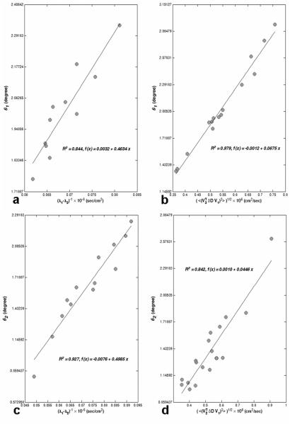
The dependence of the cone angle on the eigenvalue contrast and tensor error is shown in Fig. 5. To isolate the effect of eigenvalue contrast, we fixed other relevant parameters within narrow ranges. Under the conditions of our experiment, the coincidence angle between the major cone axis and the second principal eigenvector is near 90 degrees for the most of the white matter voxels in the ROI (Fig. 2a) as shown in Fig. 6a (this means that the upper-left element of the covariance matrix, (Σ_v1)₁₁ , in Eq. [9] is generally smaller than the lower-right element, (Σ_v1)₂₂). Therefore, we selected voxels with similar CU orientation (i.e., (Σ_v1)₁₁ < (Σ_v1)₂₂) and C_l > 0.3 (to exclude nearly isotropic voxels). For the selected voxels, a histogram of ${\epsilon }_{31}\equiv {\left[\langle {\left({\mathbf{v}}_3^{\mathrm{T}}\cdot \delta \mathbf{D}\cdot {\mathbf{v}}_1\right)}^2\rangle \right]}^{1∕2}$, the root-mean-square (RMS) error in the D₃₁ tensor element, was constructed (using N_A = 6 with 200 bootstrap samples). The peak of the histogram (i.e., the most likely value) was identified, and all voxels with ε₃₁ within 5% of this value were selected. A plot of the major cone angle (θ₁) versus (λ₁ — λ₃)^-1 for nearly constant ε₃₁ is shown in Fig. 5a. Similarly, a histogram was constructed for the eigenvalue contrast, λ₁ — λ₃ . The peak of the histogram was identified and voxels with eigenvalue contrast within 5% of this value were selected. A plot of θ₁ versus ε₃₁ for nearly constant eigenvalue contrast is shown in Fig. 5b.

Figure 5.

The major (a and b) and minor (c and d) cone angles (θ₁ and θ₂) are calculated over the ROI (Fig. 2a) and plotted as a function of the reciprocal of the eigenvalue contrast (with fixed tensor error, ε₃₁ for (a) and ε₂₁ for (c)) and as a function of the tensor error ε₃₁ for (b) and ε₂₁ for (d) (with fixed eigenvalue contrast). The slope for the linear fit is 0.4634 (a), 0.0675 (b), 0.4985 (c) and 0.0446 (d) with R² values close to one. The 95 % confidence interval for the slope is (0.31, 0.61) (a), (0.062, 0.073) (b), (0.41, 0.59) (c) and (0.035, 0.054) (d). These intervals include the nearly constant values of ε₃₁ ≅ 0.50 (a) and ε₂₁ ≅ 0.42 (c), and (λ₁ — λ₃)^-1 ≅ 0.064 (b) and (λ₁ — λ₂)^-1 ≅ 0.054 (d). Hence, the data are consistent with the relations θ₁ ≅ ε₃₁/(λ₁ — λ₃) and θ₂ ≅ ε₂₁/(λ₁ — λ₂).

Figure 6.

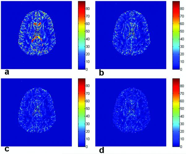
Simulated coincidence angles are shown for the whole brain slice with gradient schemes ‘original 6′ (a), ‘original 12′ (b), ‘original 21′ (c) and ‘original 92′ (d). The simulation is repeated 200 times by generating DW signals using the ‘true’ diffusion tensor with simulated random noise. The coincidence angle measures the difference in orientation between the major cone axis and the second eigenvector of the diffusion tensor (see Fig. 1b). As the number of gradient directions (i.e., angular resolution) increases, the directional coincidence increases (i.e., the coincidence angle decreases).

The two plots taken together verify the dependence of the major cone angle predicted by Eq. [15], i.e., the major cone angle should be proportional to ε₃₁ and inversely proportional to λ₁ — λ₃ . Furthermore, the slope of the line for θ₁ versus (λ₁ — λ₃)^-1 should be nearly equal to the value at the peak of the ε₃₁ histogram. Similarly, the slope of the line for θ₁ versus ε₃₁ should be nearly equal to (λ₁ — λ₃)^-1 for the peak of the eigenvalue contrast histogram. In fact, the 95% confidence interval for the slope contains the predicted value in both cases. Hence, the data are consistent with the relation θ₁/(λ₁ — λ₃) . Analogous results were obtained for the minor cone angle using ${\epsilon }_{21}\equiv {\left[\langle {\left({\mathbf{v}}_2^{\mathrm{T}}\cdot \delta \mathbf{D}\cdot {\mathbf{v}}_1\right)}^2\rangle \right]}^{1∕2}$ and (λ₁ — λ₂)^-1 (Figs. 5c and d). The predictions of first order perturbation theory and bootstrap analysis are in good agreement. However, for the conditions of this experiment both methods make the opposite assignment of major and minor cone axes relative to the case of uniform angular sampling, Eq. [15]. This is elaborated on below.

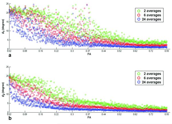
Figure 7 shows the dependence of the cone angles on FA and the number of averages (N_A). For all bootstrap samples, the maximum cone angles (N_A = 2, low FA) lie between 24 and 25 degrees and 20 to 22 degrees for the major and minor axes, respectively. With increasing numbers of averaged diffusion weighted signals (N_A = 2, 6 and 24) and FA, the directional uncertainty is reduced significantly as shown in Fig. 7.

Figure 7.

Fiber directional uncertainty quantified as cone angles for the major (θ₁ , a) and minor axis (θ₂ , b) and N_A = 2 (green), 6 (red) and 24 (blue) acquisitions with 200 bootstrap samples are shown over the ROI (Fig. 2a). The cone angle decreases with increasing N_A (i.e., SNR) and FA for both axes.

Coincidence of the tensor and v₁ covariance matrix eigenvectors

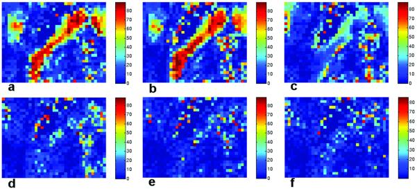
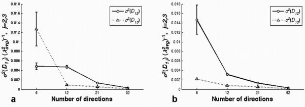
The coincidence angle is defined as the angle between the major cone axis and the second eigenvector of the ‘true’ diffusion tensor. The simulation results for all voxels in the slice are shown in Fig. 6 for four different gradient sets, ‘original 6′, ‘original 12′, ‘original 21′ and ’original 92′. Because the major and minor cone axes are orthogonal to each other and lie in the {v₂, v₃} plane, only the angle between the major cone axis and the second eigenvector is presented. In Fig. 6(a-d), most of the white matter regions have small coincidence angles, which mean the direction of the major cone axis is closer to the second than the third eigenvector of ‘true’ diffusion tensor. Especially large coincidence angles (near 90 degrees) are observed in the genu and splenium of corpus callosum in Fig. 6a using the ‘original 6′ scheme, however these also become small as the number of gradient vector directions increases, as shown in Fig. 6(b-d). Figure 8 shows the map of the coincidence angle in the ROI calculated using bootstrap and simulated data. Simulation results (Fig. 8b) based on the same gradient vector set that was used to acquire the image data agree closely with the bootstrap results (‘original 6′ with 200 sample and 6 averages; Fig. 8a). Both bootstrap (with actual noise) and Monte Carlo simulation (with modeled noise) results indicate nearly 90 degree coincidence angles in the splenium of the corpus callosum. The angular maps with the other sets (Fig. 8(c-f)), including the ‘rotated 6′ scheme, show much higher directional coincidence (small angles) across the ROI, including the same regions of the corpus callosum. This implies that coincidence angles are dependent on the number of gradient vectors (angular resolution) as well as the direction of each of the gradient vectors relative to the tensor eigenvectors. Figure 9 shows this relationship in the tensor eigenframe. The variances of the off-diagonal tensor elements (i.e., the elements that produce ${\widehat{\mathbf{v}}}_1$ errors) in the tensor eigenvector frame are shown for a representative voxel in the splenium of the corpus callosum in Fig. 9. As expected, the tensor element variances are different for the ‘original’ and ‘rotated’ gradient vector schemes at low angular resolution (hence the variation shown in Fig. 8(b-c)), but converge for high angular resolution gradient sets (as shown in Fig. 8(d-f)). The limit of infinitely many gradient directions is evaluated in the Appendix.

Figure 8.

Bootstrap and simulation coincidence angle maps for the ROI are shown. The coincidence map from the bootstrap analysis (200 samples and 6 averages) of actual data using the gradient scheme ‘original 6′ (a) is in good agreement with simulation results for the same scheme (b). Simulations show the maps of coincidence angle for other gradient schemes: ‘rotated 6′ (c), ‘original 12′ (d), ‘original 21′ (e) and ‘original 92′ (f). Coincidence angles vary as low-resolution gradient vector sets are rotated (compare b and c). As angular resolution improves, however, coincidence angles converge (d-f).

Figure 9.

Variance of the off-diagonal tensor elements, (σ² (D₁₂) and σ² (D₁₃), scaled by ${\lambda }_{\mathit{avg}}^2$ shown for a representative voxel (10^th row and 23^rd column in the ROI) in the corpus callosum for ‘original’ (a) and ‘rotated’ (b) ‘6′, ‘12′, ‘21′ and ‘92′ gradient vector schemes. These variances, along with eigenvalue contrast, determine the CU cone angles. The variances, and hence cone angles, are dependent on the gradient vector directions at low angular resolution, but converge at high angular resolution.

DISCUSSION AND CONCLUSION

In this study, we evaluated the fiber directional uncertainty using bootstrap and perturbation calculations and verified its dependence on diffusion anisotropy and SNR via time domain signal averaging. The notion of time domain averaging for measuring diffusion parameters was suggested by Skare et al. (8) as an alternative to spatial averaging schemes, as used in the Lattice Index (LI) (4,7). Time domain averaging has the obvious disadvantage of requiring more scanning time, but makes relatively few assumptions as long as a good alignment between diffusion weighted images is guaranteed. Similar improvements in fiber uncertainty are probably achievable using edge-preserving anisotropic spatial smoothing routines developed for DT-MRI (28,29).

The perturbation calculation is in good agreement with the non-parametric bootstrap analysis in estimating fiber directional uncertainty. The slope of the linear fit function and the coefficient of determination are both very close to unity regardless of image SNR. Figures 5 and 7 show that increasing either image SNR or eigenvalue contrast decreases the fiber directional error in both the major and minor axes, as theory predicts.

We tested the symmetry and normality of the CU as shown in Figs. 2c and 3. Although most of the tested CUs are significantly non-circular (Table 1 and Fig. 2c), some appeared to be nearly symmetric. Most of these near-circular cones, colored dark red in Fig. 2c, lie in the CSF or regions of likely partial volume averaging of non-parallel fibers. However, in coherent white matter voxels, the cone of uncertainty is generally non-circular. The test for multivariate normal distributions of fiber directional uncertainty is done using the multivariate skewness and kurtosis test (23,24). When we increased the number of averages from 4 to 12, the number of voxels in the ROI with normal distributions increased from 47 % to 64 % for 200 bootstrap samples. Hence, as SNR increases, the fraction of voxels with multivariate normal error increases. Most of the white matter voxels, however, have normal distributions of v₁ error regardless of the number of averages as shown in Fig. 3.

The uncertainty in the principal eigenvector is characterized by the major and minor cone angles. As shown in Figs. 4 and 7, the cone angle decreases (i.e., principal eigenvector orientation errors decrease) with increasing voxel SNR and FA. We compared the local fiber orientation when averaging N_A = 2, 6 and 24 acquisitions and using different bootstrap resampling schemes (100, 200, 500 and 1000) over a wide range of FA values (results are shown only for 200 samples). The uncertainties for both the major and minor cone axes decreased with increasing N_A and FA. However, there were no significant changes for any of the bootstrap schemes over 200 samples. The dependence on N_A in our bootstrap analysis agrees with the Monte Carlo simulations by Chang et al. (17).

Figure 5 shows the expected dependence of the cone angles on eigenvalue contrast and tensor error. The major and minor cone angles are closely predicted by the eigenvalues of the ${\widehat{\mathbf{v}}}_1$ covariance matrix, Σ_v1, defined in Eq. [9]. For the conditions of our experiment, the covariance matrix is nearly diagonal, so the diagonal values are very nearly equal to the eigenvalues. Which of the two diagonal values is larger is determined by the orientation of the gradient vector set relative to the tensor eigenframe for low angular resolution measurements. To understand this phenomenon, consider the case of low angular resolution where one diffusion weighting direction is nearly parallel to v₃ , but no measurement direction is correspondingly close to v₂ . In this case, the signal is lower for the measurement close to v₃ , so the log signal is noisier than that for v₂ (see Eq. [17] in the Appendix). The increased noise for the log signal produces larger variance in the estimated D₁₃ tensor element (see Appendix, Eqs. [22, 25]). As the number of (uniformly distributed) gradient directions increases, however, directions close to the two eigenvectors, v₂ and v₃ , are more equally sampled. In the limit of infinitely high angular resolution, the diagonal values of the v₁ covariance matrix satisfy the relation (Σ_v1)₁₁) ≥ (Σ_v1)₂₂), independent of gradient set rotation (see the Appendix). In fact this relation seems to hold for very modest angular resolution measurements. For the gradient schemes tested here, variance of the principal eigenvector in the v₂ direction was larger than the variance in the v₃ direction for all schemes with at least 12 directions (see Fig. 9). Ignoring very low angular resolution experiments for the moment, the general implication is that fiber tracking errors are always at least as large in the v₂ direction as they are in v₃ . Stated differently, the major cone axis is nearly coincident with the major axis of diffusion in the plane perpendicular to v₁.

Lazar and Alexander (13,14) described fiber tract dispersion in the plane perpendicular to the mean fiber axis using the bootstrap method. They quantified tracking errors as a function of distance from the seed point and image SNR. Their analysis showed that the distribution of tract dispersion was typically elliptical rather than circular, and there was high correlation between the direction of the major axis of the ellipse and the second eigenvector of the diffusion tensor. We verified this observation using numerical simulations (Fig. 6, 8-9) and provided a theoretical explanation for the case of many diffusion weighting directions (see the Appendix). The major axis of the ellipse is not always coincident with the second eigenvector of the tensor at very low angular resolution, for example when one of the gradient vectors is nearly parallel to the third eigenvector of the tensor. This points to an advantage of high angular resolution measurements of the tensor: the orientation of the CU is invariant under rotations of the gradient set. Taken together, the work of Lazar et al. and this study show that the statistical properties of tracking errors can be understood in terms of the cone of uncertainty. This connection has also been made recently by Koay et al. (16). The CU serves as a convenient conceptual link between local diffusion properties and the reliability of extended fiber paths. In addition, the statistical information contained in the CU can be used to make more realistic probabilistic algorithms for fiber tractography (30) and to evaluate the benefits of diffusion weighted image acquisition and gradient vector schemes for improving fiber path accuracy.

LIST OF SYMBOLS

b

Italic b

C_l

Upper case italic C, subscript l (letter ‘ell’)

D

Bold D

e₁

Bold e, subscript 1 (one)

e₂

Bold e, subscript 2

ε₃₁

Greek epsilon, subscript ‘31’

λ₁

Greek lambda, subscript 1 (one)

λ₂

Same, but subscript 2

λ₃

Same, but subscript 3

S₀

S, subscript 0 (zero)

SNR₀

SNR, subscript zero

σ₁

Greek lower case sigma, subscript one

σ₂

Greek sigma, subscript 2

σ_PT

Greek sigma, subscript ‘PT’

σ_BS

Greek sigma, subscript ‘BS’

Σ_v1

Greek upper case sigma, subscript v, sub-subscript 1 (one)

θ

Greek lower case theta

v₁

v subscript 1 (one)

v₂

v subscript 2

v₃

v subscript 3

${\widehat{\mathbf{v}}}_1$

v caret, subscript 1 (one)

APPENDIX

Eigenvector covariance in the limit of high angular resolution

We assume that the measured DTI signal in a voxel in the brain is

$$S=S_0\cdot \exp \left(-b\sum _{i,j=1}^3{n}_i{n}_j{D}_{ij}\right)+\epsilon ,$$ [16]

where S₀ is the non-diffusion weighted signal, b is the scalar diffusion weighting factor, and n_i is the i^th component of a unit vector along the diffusion weighting direction ( n₁ , n₂ , and n₃ are the x, y, and z components, respectively). The D_ij are elements of the diffusion tensor and ε a random sample of normally distributed (mean zero, variance σ²) noise. Assuming the signal-to-noise ratio in the diffusion weighted images is >> 1, this relation can be linearized as follows

$$\begin{array}{cc}\hfill S=& S_0\cdot \exp \left(-b\sum _{i,j=1}^3{n}_i{n}_j{D}_{ij}\right)\cdot \left(1+\frac{\epsilon }{\langle S\rangle }\right),\hfill \\ \hfill \ln \left(S\right)=& \ln \left(S_0\right)-b\sum _{i,j=1}^3{n}_i{n}_j{D}_{ij}+\ln \left(1+\frac{\epsilon }{\langle S\rangle }\right),\hfill \\ \hfill \cong & \ln \left(S_0\right)-b\sum _{i,j=1}^3{n}_i{n}_j{D}_{ij}+\frac{\epsilon }{\langle S\rangle }\hfill \end{array}$$ [17]

where ⟨S⟩ is the expectation value of the signal. Suppose N measurements are made using the same diffusion weighting factor, b, but different directions. Writing Eq. [17] explicitly for the k^th measurement,

$$\begin{array}{cc}\hfill \ln \left(S_k\right)\cong \ln \left(S_0\right)-b& [x_k^2{D}_{xx}+y_k^2{D}_{yy}+z_k^2{D}_{zz}+\phantom{]}\hfill \\ \hfill & \phantom{[}2x_k{y}_k{D}_{xy}+2x_k{z}_k{D}_{xz}+2y_k{z}_k{D}_{yz}]+{\eta }_k,\hfill \end{array}$$ [18]

where η_k ≡ ε_k/⟨S_k⟩ is a random variable equal to the image noise scaled by the mean signal for that measurement direction. Since the variance of η_k will generally depend on direction, a weighted least squares calculation should be used to estimate the D_ij . Let y be a column vector of elements y_k = ln(S_k) and η be a column vector of values η_k . The variables we wish to estimate can be placed in a column vector β with elements

$${\beta }^{\mathrm{T}}=\left(\ln \left(S_0\right)b{D}_{xx}b{D}_{yy}b{D}_{zz}b{D}_{xy}b{D}_{xz}b{D}_{yz}\right).$$ [19]

Finally, the design matrix, $\tilde{\mathbf{A}}$ , relates β to y . The k^th row of $\tilde{\mathbf{A}}$ is

$$A_{k:}=\left(1-x_k^2-y_k^2-z_k^2-2x_k{y}_k-2x_k{z}_k-2y_k{z}_k\right).$$ [20]

So Eq. [18] can be written simultaneously for all k as (2)

$$\mathbf{y}=\tilde{\mathbf{A}}\cdot \beta +\eta .$$ [21]

Defining a diagonal matrix $\tilde{\mathbf{V}}$ with nonzero elements equal to the signal-to-noise ratio (SNR) of the k^th measurement,

$$V_{kk}=\frac{\langle S_k\rangle }{\sigma },$$ [22]

where σ² is the variance of the ε_k , we can multiply Eq. [21] by $\tilde{\mathbf{V}}$ from the left:

$$\tilde{\mathbf{V}}\mathbf{y}=\tilde{\mathbf{V}}\tilde{\mathbf{A}}\cdot \beta +\tilde{\mathbf{V}}\eta .$$ [23]

The last term on the right is a random vector, each element of which has zero mean and unit variance. The linear least-squares solution to this uniform-variance problem is

$$\beta ={\left({\tilde{\mathbf{A}}}^{\mathbf{T}}{\tilde{\mathbf{V}}}^2\tilde{\mathbf{A}}\right)}^{-1}{\tilde{\mathbf{A}}}^{\mathbf{T}}{\tilde{\mathbf{V}}}^2\mathbf{y}.$$ [24]

The covariance matrix for β is

$${\tilde{\Sigma }}_{\beta }={\left({\tilde{\mathbf{A}}}^{\mathbf{T}}{\tilde{\mathbf{V}}}^2\tilde{\mathbf{A}}\right)}^{-1}.$$ [25]

We can use the approach of Batchelor (31) to evaluate elements of the covariance matrix in the limit of many diffusion encoding directions. Let the number of diffusion weighting directions, N, approach infinity and the directions be uniformly distributed in space. In this case, the labeling of the coordinate axes is arbitrary, so we are free to make $\widehat{z}$ (the unit vector in the Z direction) parallel to the major eigenvector, v₁ , of the tensor. Similarly, we take $\widehat{x}$ and $\widehat{y}$ in the v₂ and v₃ directions, respectively. In this coordinate system,

$$\begin{array}{cc}\hfill V_{kk}=& \frac{S_0}{\sigma }\cdot \exp \left[-b\sum _{i,j=1}^3{n}_i\left(k\right)n_j\left(k\right)D_{ij}\right]\hfill \\ \hfill =& \frac{S_0}{\sigma }\cdot \exp \left[-b\left({\lambda }_2{x}_k^2+{\lambda }_3{y}_k^2+{\lambda }_1{z}_k^2\right)\right].\hfill \end{array}$$ [26]

The first term on the right hand side is the SNR in an unweighted image. Consider the matrix

$$\begin{array}{cc}\hfill \tilde{\mathbf{M}}\equiv & \frac{4\pi }{\mathbf{N}}\cdot {\tilde{\Sigma }}_{\beta }^{-1}\hfill \\ \hfill =& \frac{4\pi }{\mathbf{N}}\cdot {\tilde{\mathbf{A}}}^{\mathbf{T}}{\tilde{\mathbf{V}}}^2\tilde{\mathbf{A}},\hfill \end{array}$$ [27]

the matrix elements of which are

$$\begin{array}{cc}\hfill M_{ij}=& \frac{4\pi }{N}\cdot \sum _{k,l=1}^N{\left({\tilde{\mathbf{A}}}^{\mathbf{T}}\right)}_{ik}{\left({\tilde{\mathbf{V}}}^2\right)}_{kl}{\left(\tilde{\mathbf{A}}\right)}_{lj}\hfill \\ \hfill =& \frac{4\pi }{N}\cdot \sum _{k=1}^N{A}_{ki}{V}_{kk}^2{A}_{kj},\hfill \end{array}$$ [28]

since $\tilde{\mathbf{V}}$ is diagonal. The sum is over diffusion weighting directions, each of which corresponds to a point (x_k,y_k,z_k) on the unit sphere. The rows of $\tilde{\mathbf{A}}$ correspond to different directions and the columns to different functions of those directions. We can write

$$A_{ki}=a_i(x_k,y_k,z_k),$$ [29]

where

$$a_i=\{\begin{array}{ccc}\hfill 1\hfill & \hfill \text{for}\hfill & \hfill i=1\hfill \\ \hfill -x^2\hfill & \hfill \hfill & \hfill i=2\hfill \\ \hfill -y^2\hfill & \hfill \hfill & \hfill i=3\hfill \\ \hfill -z^2\hfill & \hfill \hfill & \hfill i=4\hfill \\ \hfill -2xy\hfill & \hfill \hfill & \hfill i=5\hfill \\ \hfill -2xz\hfill & \hfill \hfill & \hfill i=6\hfill \\ \hfill -2yz\hfill & \hfill \hfill & \hfill i=7\hfill \end{array}\phantom{\}}.$$ [30]

Hence,

$$M_{ij}=\frac{4\pi }{N}\sum _{k=1}^N{a}_i(x_k,y_k,z_k)\cdot V_{kk}^2\cdot a_j(x_k,y_k,z_k).$$ [31]

As N → ∞ , we can define ds = 4π/N as the area on the unit sphere surrounding each measurement direction (x_k,y_k,z_k), and replace the summation in Eq. [31] with an integral over the unit sphere:

$$M_{ij}={\left(\frac{S_0}{\sigma }\right)}^2\cdot \int \int a_i(x,y,z)a_j(x,y,z)\exp [-2b({\lambda }_2{x}^2+{\lambda }_3{y}^2+{\lambda }_1{z}^2\left)\right]ds,$$ [32]

where Eq. [26] was used to substitute for V_kk. Note that the a_i for i = 1,2,3,4 and the exponential term are even functions in x, y, and z. On the other hand, the a_i for i = 5,6,7 are odd in two of the three coordinates. This implies that

$$M_{ij}=0\text{for}i\in \{1,2,3,4\}\text{and}j\in \{5,6,7\},$$ [33]

or vice versa. Hence $\tilde{\mathbf{M}}$ is block diagonal and can be written as

$$\tilde{\mathbf{M}}=\left(\begin{array}{cc}\hfill \tilde{\mathbf{P}}\hfill & \hfill {\tilde{0}}_{4\times 3}\hfill \\ \hfill {\tilde{0}}_{3\times 4}\hfill & \hfill \tilde{\mathbf{Q}}\hfill \end{array}\right),$$ [34]

where $\tilde{\mathbf{P}}$ is 4×4, $\tilde{\mathbf{Q}}$ is 3×3 ${\tilde{0}}_{n\times m}$ is an n×m matrix of zeros. Furthermore, $\tilde{\mathbf{Q}}$ is diagonal, since the product of any two of the functions xy, xz, and yz is also odd in two of the coordinates. The diagonal elements of $\tilde{\mathbf{Q}}$ are

$$Q_{11}={\left(\frac{2S_0}{\sigma }\right)}^2\cdot \int \int x^2{y}^2\exp \left[-2b\left({\lambda }_2{x}^2+{\lambda }_3{y}^2+{\lambda }_1{z}^2\right)\right]ds,$$ [35]

$$Q_{22}={\left(\frac{2S_0}{\sigma }\right)}^2\cdot \int \int x^2{z}^2\exp \left[-2b\left({\lambda }_2{x}^2+{\lambda }_3{y}^2+{\lambda }_1{z}^2\right)\right]ds,$$ [36]

$$Q_{33}={\left(\frac{2S_0}{\sigma }\right)}^2\cdot \int \int y^2{z}^2\exp \left[-2b\left({\lambda }_2{x}^2+{\lambda }_3{y}^2+{\lambda }_1{z}^2\right)\right]ds.$$ [37]

Next, we show that Q₃₃ ≥ Q₂₂. We can rewrite the Q_ii explicitly in terms of the polar and azimuthal angles, θ and φ , describing each diffusion weighting direction. First, note that

$$\begin{array}{cc}\hfill {\lambda }_2{x}^2+{\lambda }_3{y}^2+{\lambda }_1{z}^2=& {\lambda }_2{\cos }^2\varphi {\sin }^2\theta +{\lambda }_3{\sin }^2\varphi {\sin }^2\theta +{\lambda }_1{\cos }^2\theta \hfill \\ \hfill =& {\lambda }_2{\cos }^2\varphi {\sin }^2\theta +{\lambda }_3\left(1-{\cos }^2\varphi \right){\sin }^2\theta +{\lambda }_1\left(1-{\sin }^2\theta \right).\hfill \\ \hfill =& {\lambda }_1+{\sin }^2\theta \left[\left({\lambda }_2-{\lambda }_3\right){\cos }^2\varphi -({\lambda }_1-{\lambda }_3)\right]\hfill \end{array}$$ [38]

Hence the lower two diagonal elements are

$$\begin{array}{c}\hfill Q_{22}={\left(\frac{2S_0}{\sigma }\right)}^2\cdot {\int }_0^{\pi }\left[{\int }_0^{2\pi }{\cos }^2\varphi \exp \{-2b{\sin }^2\theta {\cos }^2\varphi ({\lambda }_2-{\lambda }_3\left)\right\}d\varphi \right].\hfill \\ \hfill {\sin }^3\theta {\cos }^2\theta \exp \{-2b\left[{\lambda }_1-{\sin }^2\theta \left({\lambda }_1-{\lambda }_3\right)\right]\}d\theta ,\hfill \end{array}$$ [39]

$$\begin{array}{c}\hfill Q_{33}={\left(\frac{2S_0}{\sigma }\right)}^2\cdot {\int }_0^{\pi }\left[{\int }_0^{2\pi }{\sin }^2\varphi \exp \{-2b{\sin }^2\theta {\cos }^2\varphi ({\lambda }_2-{\lambda }_3\left)\right\}d\varphi \right].\hfill \\ \hfill {\sin }^3\theta {\cos }^2\theta \exp \{-2b\left[{\lambda }_1-{\sin }^2\theta \left({\lambda }_1-{\lambda }_3\right)\right]\}d\theta ,\hfill \end{array}$$ [40]

These differ only in the φ integrals. The φ integrals for Q₂₂ and Q₃₃ are

$$H_{22}\left(\alpha \right)\equiv {\int }_0^{2\pi }{\cos }^2\varphi \cdot e^{-\alpha \cdot {\cos }^2\varphi }d\varphi ,$$ [41]

$$H_{33}\left(\alpha \right)\equiv {\int }_0^{2\pi }{\sin }^2\varphi \cdot e^{-\alpha \cdot {\cos }^2\varphi }d\varphi ,$$ [42]

respectively, with α = 2b(λ₂ — λ₃)sin² θ≥0. These integrals can be expressed as modified Bessel functions using the relation

$$I_0\left(z\right)=\frac{1}{\pi }{\int }_0^{\pi }{e}^{\pm z\cdot \cos {\varphi }^{\prime }}d{\varphi }^{\prime }$$ [43]

I₀ (z) is the modified Bessel functions of order zero. Making the change of variables to φ = φ’/2 and using the half angle relation cos(2φ) = 2cos²φ—1 we have

$$\begin{array}{cc}\hfill I_0\left(z\right)=& 2\frac{e^z}{\pi }\cdot {\int }_0^{\pi ∕2}{e}^{-2z{\cos }^2\varphi }d\varphi \hfill \\ \hfill =& \frac{e^z}{2\pi }\cdot {\int }_0^{2\pi }{e}^{-2z{\cos }^2\varphi }d\varphi .\hfill \end{array}$$ [44]

Hence

$$I_0(z∕2)=\frac{e^{z∕2}}{2\pi }\cdot {\int }_0^{2\pi }{e}^{-z\cdot {\cos }^2\varphi }d\varphi .$$ [45]

Differentiating both sides of this relation with respect to z gives

$$\frac{d}{dz}{I}_0(z∕2)=\frac{e^{z∕2}}{4\pi }\cdot {\int }_0^{2\pi }{e}^{-z\cdot {\cos }^2\varphi }d\varphi -\frac{e^{z∕2}}{2\pi }\cdot {\int }_0^{2\pi }{\cos }^2\varphi \cdot e^{-z\cdot {\cos }^2\varphi }d\varphi .$$ [46]

The zero order modified Bessel function obeys the relation

$$\frac{d}{dz}{I}_0\left(z\right)=I_1\left(z\right),$$ [47]

where I₁ (z) is the first order modified Bessel function. Using this relation and Eq. [45] in Eq. [46], we have

$$\frac{1}{2}{I}_1(z∕2)=\frac{1}{2}{I}_0(z∕2)-\frac{e^{z∕2}}{2\pi }\cdot {\int }_0^{2\pi }{\cos }^2\varphi \cdot e^{-z\cdot {\cos }^2\varphi }d\varphi ,$$ [48]

or

$${\int }_0^{2\pi }{\cos }^2\varphi \cdot e^{-z\cdot {\cos }^2\varphi }d\varphi =\pi e^{-z∕2}\left[I_0(z∕2)-I_1(z∕2)\right].$$ [49]

Similarly,

$$\begin{array}{cc}\hfill {\int }_0^{2\pi }{\sin }^2\varphi \cdot e^{-z\cdot {\cos }^2\varphi }d\varphi =& {\int }_0^{2\pi }\left(1-{\cos }^2\varphi \right)\cdot e^{-z\cdot {\cos }^2\varphi }d\varphi \hfill \\ \hfill =& {\int }_0^{2\pi }{e}^{-z\cdot {\cos }^2\varphi }d\varphi -{\int }_0^{2\pi }{\cos }^2\varphi \cdot e^{-z\cdot {\cos }^2\varphi }d\varphi \hfill \\ \hfill =& 2\pi e^{-z∕2}{I}_0(z∕2)-\pi e^{-z∕2}\left[I_0(z∕2)-I_1(z∕2)\right]\hfill \\ \hfill =& \pi e^{-z∕2}\left[I_0(z∕2)+I_1(z∕2)\right],\hfill \end{array}$$ [50]

using Eqs. [45] and [49] on the second line. Substituting Eqs. [49] and [50] in Eq. [41] and [42], respectively,

$$H_{22}\left(\alpha \right)\equiv \pi e^{-\alpha ∕2}\left[I_0(\alpha ∕2)-I_1(\alpha ∕2)\right],$$ [51]

$$H_{33}\left(\alpha \right)\equiv \pi e^{-\alpha ∕2}\left[I_0(\alpha ∕2)-I_1(\alpha ∕2)\right].$$ [52]

Since the modified Bessel functions are real and positive for α ≥ 0 , we have

$$H_{33}\left(\alpha \right)\ge H_{22}\left(\alpha \right).$$ [53]

The equality holds if and only if α = 0 (since I₁ (0) = 0). Because these terms are the only difference between the integrands of Q₂₂ and Q₃₃ (and the integrands are non-negative), we have

$$Q_{33}\ge Q_{22}.$$ [54]

For the case of interest ( b > 0) the equality holds only when λ₂ = λ₃.

Since the matrix $\tilde{\mathbf{M}}$ is block diagonal (Eq. [34]), its inverse is also block diagonal:

$${\tilde{\mathbf{M}}}^{-1}=\left(\begin{array}{cc}\hfill {\tilde{\mathbf{P}}}^{-1}\hfill & \hfill {\tilde{0}}_{4\times 3}\hfill \\ \hfill {\tilde{0}}_{3\times 4}\hfill & \hfill {\tilde{\mathbf{Q}}}^{-1}\hfill \end{array}\right),$$ [55]

and since $\tilde{\mathbf{Q}}$ is diagonal,

$${\tilde{\mathbf{Q}}}^{-1}=\left(\begin{array}{ccc}\hfill \frac{1}{Q_{11}}\hfill & \hfill 0\hfill & \hfill 0\hfill \\ \hfill 0\hfill & \hfill \frac{1}{Q_{22}}\hfill & \hfill 0\hfill \\ \hfill 0\hfill & \hfill 0\hfill & \hfill \frac{1}{Q_{33}}\hfill \end{array}\right).$$ [56]

Substituting Eqs. [55] and [56] into Eq. [27] and solving for the covariance matrix, we find

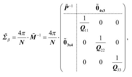[57]

where

$$\frac{1}{Q_{22}}\ge \frac{1}{Q_{33}}.$$ [58]

Referring to the order of tensor elements in Eq. [19], this shows that the variance of D_xz is greater than or equal to the variance of D_yz. In terms of the principal axis indices, we have

$${\sigma }^2\left(D_{12}\right)\ge {\sigma }^2\left(D_{13}\right).$$ [59]

The equality holds only when λ₂ = λ₃ . Further, since the lower-right block of ${\tilde{\Sigma }}_{\beta }$ is diagonal, the errors in D₁₂ are uncorrelated with errors in D₁₃. A similar calculation shows that the same results hold if the tensor is calculated using standard (unweighted) linear least squares estimation. To summarize, in the case of many, uniformly distributed measurement directions and λ₂ > λ₃, the errors in D₁₂ are larger than the errors in D₁₃, and the two are uncorrelated.

REFERENCES

- 1.Basser PJ, Mattiello J, LeBihan D. MR diffusion tensor spectroscopy and imaging. Biophys J. 1994;66:259–267. doi: 10.1016/S0006-3495(94)80775-1. [DOI] [PMC free article] [PubMed] [Google Scholar]
- 2.Basser PJ, Mattiello J, LeBihan D. Estimation of the effective self-diffusion tensor from the NMR spin echo. J Magn Reson B. 1994;103:247–254. doi: 10.1006/jmrb.1994.1037. [DOI] [PubMed] [Google Scholar]
- 3.Basser PJ, Pierpaoli C. Microstructural and physiological features of tissues elucidated by quantitative-diffusion-tensor MRI. J Magn Reson B. 1996;111:209–219. doi: 10.1006/jmrb.1996.0086. [DOI] [PubMed] [Google Scholar]
- 4.Pierpaoli C, Jezzard P, Basser PJ, Barnett A, Di Chiro G. Diffusion tensor MR imaging of the human brain. Radiology. 1996;201:637–648. doi: 10.1148/radiology.201.3.8939209. [DOI] [PubMed] [Google Scholar]
- 5.Mori S, Crain BJ, Chacko VP, van Zijl PC. Three-dimensional tracking of axonal projections in the brain by magnetic resonance imaging. Ann Neurol. 1999;45:265–269. doi: 10.1002/1531-8249(199902)45:2<265::aid-ana21>3.0.co;2-3. [DOI] [PubMed] [Google Scholar]
- 6.Bastin ME, Armitage PA, Marshall I. A theoretical study of the effect of experimental noise on the measurement of anisotropy in diffusion imaging. Magn Reson Imag. 1998;16:773–785. doi: 10.1016/s0730-725x(98)00098-8. [DOI] [PubMed] [Google Scholar]
- 7.Pierpaoli C, Basser PJ. Toward a quantitative assessment of diffusion anisotropy. Magn Reson Med. 1996;36:893–906. doi: 10.1002/mrm.1910360612. [DOI] [PubMed] [Google Scholar]
- 8.Skare S, Li TQ, Nordell B, Ingvar M. Noise considerations in the determination of diffusion tensor anisotropy. Magn Reson Imag. 2000;18:659–669. doi: 10.1016/s0730-725x(00)00153-3. [DOI] [PubMed] [Google Scholar]
- 9.Basser PJ, Pajevic S. Statistical artifacts in diffusion tensor MRI (DT-MRI) caused by background noise. Magn Reson Med. 2000;44:41–50. doi: 10.1002/1522-2594(200007)44:1<41::aid-mrm8>3.0.co;2-o. [DOI] [PubMed] [Google Scholar]
- 10.Anderson AW. Theoretical analysis of the effects of noise on diffusion tensor imaging. Magn Reson Med. 2001;46:1174–1188. doi: 10.1002/mrm.1315. [DOI] [PubMed] [Google Scholar]
- 11.Basser PJ. Quantifying errors in fiber-tract direction and diffusion tensor field maps resulting from MR noise. Proceedings of the 5th Annual Meeting of ISMRM; Vancouver, Canada: 1997. p. 1740. [Google Scholar]
- 12.Jones DK. Determining and visualizing uncertainty in estimates of fiber orientation from diffusion tensor MRI. Magn Reson Med. 2003;49:7–12. doi: 10.1002/mrm.10331. [DOI] [PubMed] [Google Scholar]
- 13.Lazar M, Alexander AL. Bootstrap white matter tractography (BOOT-TRAC) NeuroImage. 2005;24:524–532. doi: 10.1016/j.neuroimage.2004.08.050. [DOI] [PubMed] [Google Scholar]
- 14.Lazar M, Lee JH, Alexander AL. Axial asymmetry of water diffusion in brain white matter. Magn Reson Med. 2005;54:860–867. doi: 10.1002/mrm.20653. [DOI] [PubMed] [Google Scholar]
- 15.Jeong H-K, Lu Y, Ding Z, Anderson AW. Characterizing cone of uncertainty in diffusion tensor MRI. Proceedings of the 13th Annual Meeting of ISMRM; Miami Beach, USA: 2005. p. 1317. [Google Scholar]
- 16.Koay C, Chang L-C, Basser PJ. The Cone of Uncertainty is Elliptical: Implications for DTI Tractography. Proceedings of the 15th Annual Meeting of ISMRM; Berlin, Germany: 2007. p. 1602. [Google Scholar]
- 17.Chang LC, Koay CG, Pierpaoli C, Basser PJ. Variance of estimated DTI-derived parameters via first-order perturbation methods. Magn Reson Med. 2007;57:141–149. doi: 10.1002/mrm.21111. [DOI] [PubMed] [Google Scholar]
- 18.Hext GR. The estimation of second-order tensors, with related tests and designs. Biometrika. 1963;50:353–373. [Google Scholar]
- 19.Johnson RA, Wichern DW. Applied multivariate statistical analysis. 4th ed Prentice Hall; New Jersey: 1998. pp. 160–164. [Google Scholar]
- 20.Basser PJ, Pierpaoli C. A simplified method to measure the diffusion tensor from seven MR images. Magn Reson Med. 1998;39:928–934. doi: 10.1002/mrm.1910390610. [DOI] [PubMed] [Google Scholar]
- 21.Efron B. Bootstrap methods: another look at the jackknife. Ann Statist. 1979;7:1–26. [Google Scholar]
- 22.Jackson JE. A user’s guide to principal components. John WiIey & Sons; New York: 1991. p. 33. [Google Scholar]
- 23.Mardia KV. Measures of multivariate skewness and kurtosis with applications. Biometrika. 1970;57:519–530. [Google Scholar]
- 24.Mardia KV, Kent JT, Bibby JM. Multivariate analysis. Academic Press; New York: 1979. p. 148. [Google Scholar]
- 25.Papadakis NG, Xing D, Huang CL-H, Hall LD, Carpenter A. A comparative study of acquisition schemes for diffusion tensor imaging using MRI. J Magn Reson. 1999;137:67–82. doi: 10.1006/jmre.1998.1673. [DOI] [PubMed] [Google Scholar]
- 26.Wolfram S. The Mathematica Book. 3rd ed Wolfram Media/Cambridge University Press; Champaign, IL: 1996. [Google Scholar]
- 27.Westin C-F, Peled S, Gudbjartsson H, Kikinis R, Jolesz FA. Geometrical diffusion measures for MRI from tensor basis analysis. Proceedings of the 5th Annual Meeting of the ISMRM; Vancouver, Canada: 1997. p. 1742. 1997. [Google Scholar]
- 28.Ding Z, Gore JC, Anderson AW. Reduction of noise in diffusion tensor images using anisotropic smoothing. Magn Reson Med. 2005;53:485–490. doi: 10.1002/mrm.20339. [DOI] [PubMed] [Google Scholar]
- 29.Chen B, Hsu EW. Noise removal in magnetic resonance diffusion tensor imaging. Magn Reson Med. 2005;54:393–407. doi: 10.1002/mrm.20582. [DOI] [PubMed] [Google Scholar]
- 30.Lu Y, Aldroubi A, Gore JC, Anderson AW, Ding Z. Improved fiber tractography with Bayesian tensor regularization. NeuroImage. 2006;31:1061–1074. doi: 10.1016/j.neuroimage.2006.01.043. [DOI] [PubMed] [Google Scholar]
- 31.Batchelor PG, Atkinson D, Hill DL, Calamante F, Connelly A. Anisotropic noise propagation in diffusion tensor MRI sampling schemes. Magn Reson Med. 2003;49:1143–1151. doi: 10.1002/mrm.10491. [DOI] [PubMed] [Google Scholar]