

Abstract
Two algorithms for simulating the response of peptides to sequences of infrared pulses are developed and applied to N-methyl acetamide (NMA) and a 17 residue alpha helical peptide (YKKKH17) in D2O. A fluctuating vibrational-exciton Hamiltonian for the amide I mode is constructed from MD trajectories. Coupling with the environment is described using a DFT electrostatic map. The Cumulant expansion of Gaussian Fluctuation (CGF) incorporates motional narrowing due to fast frequency fluctuations and is adequate for NMA and for isotopically labelled bands in large peptides. Real-space truncation of the scattering matrix of the Nonlinear Exciton Equations (NEE) significantly reduces the computational cost, making it particularly attractive for slow fluctuations in large globular proteins.
I. Introduction
Probing the structure and folding dynamics of proteins is one of the most fundamental problems in biophysics and has been the subject of intensive effort [1–16]. Infrared spectroscopy provides a valuable tool in these studies [17–24]. Significant progress has been made over the past decade in developing coherent two-dimensional infrared (2DIR) techniques [25–33]. In a 2DIR experiment three incoming pulses with wavevectors k1, k2, and k3 interact with the peptide to generate a coherent signal in one of the directions ks = ±k1 ± k2 ± k3. The pulse sequence and time delays (t1,t2, and t3) are shown in Fig. 1. Two-dimensional correlation plots of the signals plotted as fourier transforms with respect to two of these delay periods reveal new types of information with enhanced spectral resolution. Diagonal peaks show the fundamental transitions, while cross peaks and their lineshapes probe the fluctuations of the correlations among various structural elements [26].
FIG. 1.
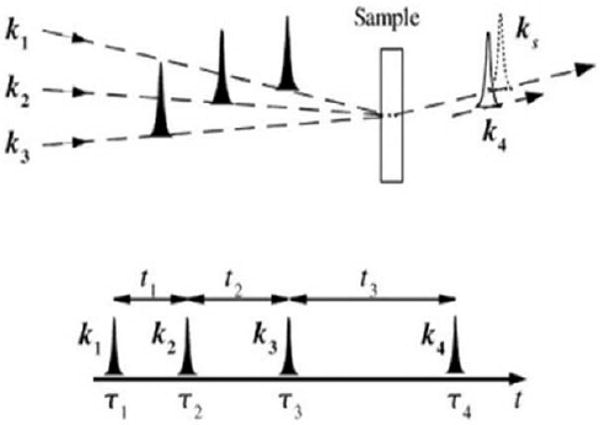
(top) pulse configuration for heterodyne four wave mixing. k1, k2, k3 are the input pulses, ks is the signal generated, which is in the same direction as the detection pulse k4. (bottom) the pulse sequence for coherent 2D experiments. tj are the time intervals between pulses centered at τi.
Two-dimensional NMR techniques originally introduced in the seventies [34] had turned it into a useful structural tool [35]. Extracting information from NMR data requires extensive simulations. The “direct inversion” of spectra to structures is based on constrained fits guided by simulations[36–38]. A recent study of human ubiquitin in solution [37] had combined NMR experiments with MD simulations to directly determine the entire ensembles of protein conformations, rather than merely the average structure: Both the native structure and its associated dynamics are thus obtained simultaneously. Since infrared spectra are more congested, and anharmonic vibrational hamiltonians are much more complex than spin hamiltonians [39, 40], efficient simulation strategies are essential for the interpretation and analysis of 2DIR signals. Thanks to the ultrafast timescale, the simulation of 2DIR signals with atomic level details only requires sub-nanosecond trajectories, which are readily available[41–44].
Standard tools are available for computing two-point correlation functions which are commonly used in the analysis of fluctuations. Nonlinear response functions require the efficient and accurate sampling of multipoint correlation functions; This article addresses some of the simulation challenges involved in predicting and interpreting Multidimensional measurements.
We focus on the amide vibrational modes which are localized along the peptide backbone. Their couplings (∼ 10cm−1) which depend on the secondary structure and its fluctuations, are typically much smaller than the mode frequencies (∼ 1600cm−1). The spectrum thus consists of well-separated groups of energy levels representing single excitations |e >, double excitations |f >, etc.,(Fig. 4 (vi)). The laser pulses probe the system by inducing transitions among these manifolds. Linear (single pulse) techniques only access the lowest (single-exciton) manifold, whereas doubly excited (two-exciton) states can be effectively monitored by third-order spectroscopies.
FIG. 4.
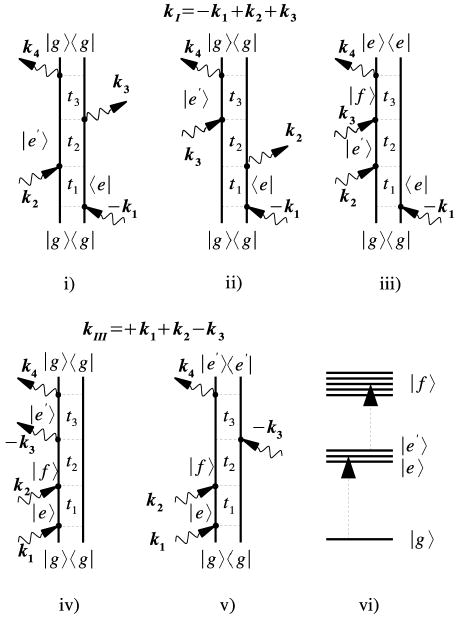
Double-sided Feynman diagrams for the kI and kIII techniques showing the pulse sequence and the vibrational density matrix during each time interval.
Spectra of small peptides may be calculated using sum-over-states (SOS) expressions [45] in conjunction with simulated structural trajectories. The optical response is described in terms of transitions among eigenstates. For short peptides, in which level crossings among eigenstates can be ignored, the Cumulant expansion of Gaussian Fluctuation (CGF) [45] can be adopted to account for bath fluctuations of arbitrary timescale, ranging from motional narrowing(fast), to the inhomogeneous broadening regime (slow). For several reasons, a different simulation protocol should be adopted for large peptides: The SOS computational cost of third order coherent signals scales as ∼ N4 [45], where N is the number of coupled oscillators, and this calculation becomes prohibitively expensive as N is increased. In addition, as the peptide size is increased, the energy levels become more dense, and the adiabatic approximation underlying the CGF no longer holds. Finally, in large peptides, the spectra are often dominated by slow large-scale structural fluctuations. Line broadening may then be simulated by averaging the homogeneous response over ensembles of system configurations [46].
The Nonlinear Exciton Equations (NEE) [45, 47–49] provide a practical alternative for large proteins. These equations use the single-exciton basis and view the nonlinear response in terms of scattering among one-exciton quasiparticles. Two-exciton resonances enter through the exciton scattering matrix, totally avoiding the expensive computation of multiple exciton states. The apparent NEE scaling of the computational cost for third order signals is also ∼ N4, similar to the SOS. however, by exploiting the short range nature of exciton couplings, the cost may be reduced considerably and could even scale linearly with protein size.
We explore the applicability and test the limits of the CGF and NEE formalisms. Linear absorption and several third order signals are predicted and discussed for the amide I band lineshape of N-methyl acetamide (NMA) and a 17 residue alpha helical peptide Ac–YAAKAAAAKAAAAKAAH–NH2 (named YKKKH17 since YKKKH are its non-alanine (lysine) residues) in D2O (lower panel of Fig. 2). We demonstrate that the CGF is suitable for NMA and for narrow isotopically labelled bands whereas the NEE with inhomogeneous averaging yields accurate spectra for large peptides.
FIG. 2.
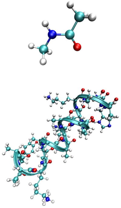
The structure of NMA (top) and YKKKH17 (bottom).
A brief survey of coherent multidimentional signals is given in section II, more details can be found in [29, 50]. An accurate vibrational exciton Hamiltonian is crucial for the simulation of spectra. An electrostatic DFT map is constructed for the fundamental frequencies and anharmonicities and used to generate the hamiltonian of NMA [51]. The vibrational Hamiltonian is introduced in section III, and the simulation protocols are outlined in section IV and presented in detail in section V (CGF) and VI (NEE). These are then applied to NMA (section VII) and YKKKH17 (section VIII). We finally discuss our results and future applications in section IX.
II. Coherent Multidimentional Signals of Coupled Vibrations
We consider third order signals induced by three resonant femtosecond pulses with the electric field:
| (1) |
where E(j) is the amplitude of the j'th pulse, and νj = x, y, z denotes its polarization direction.
We assume an ideal impulsive experiment with very short pulses where the desired time ordering of the various interactions is enforced. Finite-pulse envelopes can be included [50] but the experiment is best understood in this impulsive limit. The response of an ensemble of molecules is determined by the nonlinear polarization [50], P, which serves as the source for the ks signal in the Maxwell equations:
| (2) |
The system is initially at equilibrium in the ground state, and the response function depends parameterically on the three time intervals between pulses tj (Fig. 1). Due to interference of the induced polarization of the various molecules, the signal is only generated along specific (phase matching) directions ks. There are four possible signals with wavevectors: kI = − k1 + k2 + k3, kII = + k1 − k2 + k3, kIII = + k1 + k2 − k3 and kIV = + k1 + k2 + k3. These techniques can be understood by using Feynman diagrams [50] which depict the evolution of the vibrational density matrix in the course of the nonlinear process. (Fig. 4). Time goes from the bottom to the top, the two vertical lines in the diagram represent the ket and the bra of the density matrix, while arrows represent interactions with the laser pulses.
We shall focus on kI and kIII. The three diagrams contributing to kI are shown in Fig. 4 (top). In all diagrams the density matrix is in a single-quantum coherence |g >< e| between the ground state and the singly excited state during t1. During t3 it is either in the conjugate coherence |e >< g| ((i) and (ii)), or in a coherence between the one and two exciton manifolds |f >< e| (iii). The kI signal is displayed by performing a double Fourier transform with respect to the first and the third time delays ( ):
| (3) |
where Ω1 and Ω3 are the fourier conjugates to t1 and t3 respectively. In all calculations, we set t2 = 0.
kIII is similarly described by the two Feynman diagrams (iv) and (v) and shows double-quantum coherences between ground state and the two–exciton band |f >< g| during the t2 interval. During t3 it has a single quantum coherence |e′ >< g| (iv) and |f >< e′| (v). kI, known as the photon echo, can improve the resolution by eliminating certain types of inhomogeneous broadening. The spectral bandwidth is doubled in kIII which carries direct information regarding the coherence between the two exciton states and the ground state (double quantum coherence) [28]. The system is transferred to a coherence by the first pulse. The second pulse takes the system either to a population or to a coherence between two excitonic states. Then the population and coherence evolution can be probed by holding the second delay time, t2 (often referred to as population waiting time) fixed. The third pulse creates coherences either between the ground and one-exciton states or between one- and two-exciton states.
By performing a Fourier transforms with respect to the second and the third time delays (Ω2 and Ω3 are the fourier conjugates to t2 and t3 respectively) we can observe double (single) quantum coherence along Ω2 (Ω3). The kIII signal is:
| (4) |
In all the calculations we have set t1 = 0 is set to zero.
The linear response is similarly related to the linear response function:
| (5) |
whose fourier transform gives the absorption spectrum:
| (6) |
III. The Fluctuating Vibrational-Exciton Hamiltonian
The construction of a fluctuating hamiltonian for the primary vibrations and their coupling with a bath is the first step in the simulation of vibrational lineshapes. Nonlinear signals are sensitive to fine details (e.g. anharmonicities, overtone transitions.. etc.,) and require a high-level hamiltonian [52]. Vibrational motions and spectra are commonly described by normal modes. These collective coordinates provide a convenient zero-order approximation for the vibrational eigenstates and frequencies. However, a normal mode analysis is not required and is often too expensive for large polypeptides. Instead, since the amide I vibrations are localized on the backbone peptide bonds, it is desirable to trace the structural origin of spectral features to local vibrational coordinates [53]. A peptide can be viewed as a chain of beads, each containing one amide residue (O=C-N-H). The Frenkel exciton model has long been used [17, 19, 54, 55] to represent the vibrational hamiltonian in this localized basis. Diagonal elements of the hamiltonian matrix give the zero-order local mode frequencies while off-diagonal elements represent their couplings. For large globular proteins, the hamiltonian may be constructed using parameters obtained from quantum chemistry calculations performed on small segments.
Quantum calculations of 96 NMA-water clusters were recently combined with a fitting procedure to obtain a linear relation between the frequency of NMA, a simplest model system for the peptide bond, and the instant external electric potential[56]. A similar procedure was adopted to obtain a relation between NMA frequency and the external electric fields from 200 cluster calculations [57]. Both approaches work very well for the absorption linewidth (27 cm−1, compared with experimental width 29 cm−1) and give a reasonable solvent peak shift (60cm−1 compared with experimental shift 90cm−1). By considering some of the extreme configurations of NMA-water clusters, Keiderling reproduced the solvent shift even better [58].
The cluster fitting for specific solvents is highly accurate but may be too expensive for applications which require repeated calculations for large number of configurations of complex polypeptides. We thus adopt a different approach, starting with the vibrational exciton Hamiltonian:
| (7) |
where
| (8) |
is the system Hamiltonian and ĤF is the interaction with the optical field, E(t):
| (9) |
(B̂m) is the creation (annihilation) operator for the m'th amide I mode, localized within the amide unit (O=C-N-H), with frequency εm, anharmonicity Δm and transition dipole moment μm. These operators satisfy the Bose commutation relations . Jmn are the harmonic inter-mode couplings. All parameters of ĤS fluctuate due to conformational changes of the backbone, the solvent and side-chain dynamics.
To describe the m'th localized amide I mode it must be separated from all other modes: the segment made of that amide residue and two neighboring neutral groups (according to CHARMM27 force field [44], which we use in electrostatic interaction calculation) containing the α carbons is defined as the chromophore (Fig 3). The rest of the protein, i.e., all atoms other than this chromophore, and the solvent molecules are treated as a bath, whose effect on the chromophore will be described by a fluctuating electrostatic field.
FIG. 3.
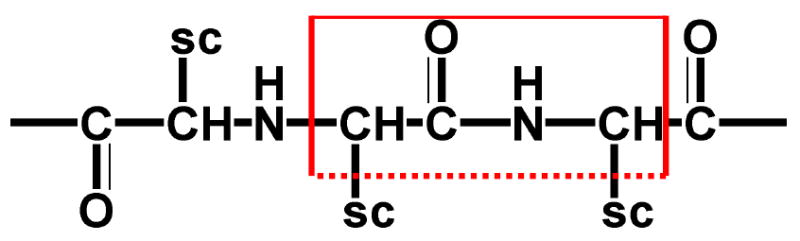
The amide I vibrational chromophore (red rectangle). “SC” stands for “side chain”. the dotted line at the bottom indicates that some atoms of the side chain may be included in the chromophore depending on the “group” defined in the charmm force field.
The frequency of mode m subjected to by a time dependent electric field is given by εm(E) = ε − δεm(E). ε = 1717cm−1 is the frequency of an isolated NMA in the gas phase [58]. The spectral shift δεm(E) and the anharmonicity Δm(E) are obtained from an ab initio DFT map which relates the electric field and its derivatives at a reference point to the fundamental and overtone frequencies of the amide I mode [51]. Geometry optimization was performed on a gas phase NMA reference structure at the BPW91/6-31g(d,p) level of DFT using GAUSSIAN03 [59]. This functional is known to give accurate vibrational frequencies [58]. During optimization, the origin is set to be in the middle of the line connecting Oxygen and Hydrogen atoms of this NMA molecule, and the x axis goes from O to H. O=C-N-H then define the x-y plane, where the y axis points towards the N atom. The mid point of the carbonyl oxygen and the amide Hydrogen of the reference structure was chosen as a reference point.
A DFT map was constructed which relates δεm(E) and Δm(E) to a 19 component vector CT ≡ (Ex, Ey, Ez, Exx, ⋯, Exxx, ⋯) representing all independent components of the electric field, its gradients and second derivatives at the reference point [60]:
| (10) |
The coefficients Kν and Kνν′ are obtained from vibrational eigenstate calculations for the sixth order DFT anharmonic vibrational potential of a single NMA chromophore in a spatially nonuniform electric field [51]. Δm(E) was expanded in a similar fashion. A modified Gaussian 03 code was used to generate the anharmonic potential and the ARNOLDI algorithm was employed for the eigenstates calculations. To trace the origin of electric field influence on the amide I band, the C=O bond length obtained by energy minimization for the various field values was also parametrized in terms of C [51].
The instantaneous C=O bond length was calculated from the DFT map. The scatter plot of the amide I frequency versus C=O bond length is shown in Fig. 5. The strong positive correlation suggests that electric field fluctuation causes geometrical changes of the amide unit due to polarization, which is the reason of the amide I frequency fluctuation. This agrees with the conclusions from previous studies [51, 61–63].
FIG. 5.
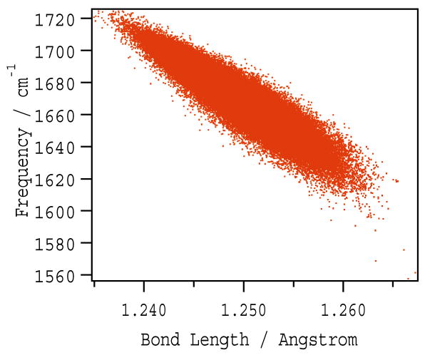
Scatter plots of amide I fundamental frequency versus the C=O bond length.
To identify the spatial region of the electric field relevant in the amide vibrations, we have expanded the molecular charge density ρ(r) in the vibrational modes Qi:
| (11) |
The transition charge density (TCD) ∂ρ/∂Q [51] represents the electronic structure change due to the Qi vibration. We expect the electrostatic potential generated by the solvent in the region where the TCD is large to dominate the optical response of that vibration. Three electric field components sampled at 67 points in space spaning the transition charge density region of the amide mode were calculated for each bath configuration. The components of CT were determined at each time point by a least-square fit to the electric field sampled at these 67 points. CT calculated using this protocol represents the electric field distribution across the transition charge density region.
The couplings of different amide modes were assumed to depend solely on the peptide backbone structure. For nearest covalently-bonded modes we used Torii and Tasumi's abinitio map [20]. All other couplings were calculated by making the dipole approximation for each amide unit [17, 19] and using the electrostatic Transition Dipole Coupling (TDC) model:
| (12) |
where μm is the transition dipole in (D Å−1 u−1/2) units, rmn is the distance between dipoles (in Å), emn is the unit vector connecting m and n and ε = 1 is the dielectric constant. The angle between the transition dipole and C=O bond is 10 degrees. A = 848619/1650 is a conversion factor which gives the coupling energy in cm−1.
IV. The Simulation Protocols
The CGF modelling of the coherent vibrational response involves the following steps:
A molecular dynamics simulation generates a sequence of protein and solvent configurations for NMA and YKKKH17.
A fluctuating vibrational-exciton hamiltonian, ĤS(t), and the transition dipole matrix, μ(t), in the one-exciton and two-exciton basis are constructed for each configuration. The fundamental frequencies and the diagonal anharmonicities are generated by our electrostatic DFT map [51].
The reference exciton Hamiltonian H̄S is obtained as the time average of ĤS(t). The eigenvalues, ω̄n, and eigenvectors, ψ̄n, of this Hamiltonian form a reference basis. The trajectory of ĤS(t) and μ(t) is transformed to the reference basis set, creating a fluctuating Hamiltonian matrix with δωn(t) = ωn(t) − ω̄n, (diagonal fluctuations) and off-diagonal fluctuations of couplings, δJmn(t) ≡ Jmn(t). The line broadening functions (eq. 15) were generated using this Hamiltonian.
The necessary products of four transition dipoles are calculated. Both orientational averaging [64] and a time averaging were performed to account for fluctuations of the transition dipoles.
The Reference Hamiltonian, line broadening functions and average amplitudes of the Liouville space pathways were combined to calculate the response functions. Experimental lifetime broadening is added [65].
The NEE approach requires the following steps:
An MD or a Monte Carlo simulation generates an ensemble of system configurations.
The fluctuating vibrational exciton hamiltonian, ĤS(t), and trasition dipole matrix, μ(t) were constructed in a similar fashion to the CGF, except that only the one exciton block is calculated.
At each configuration we used ĤS(t) to calculate the exciton scattering matrix in the one-exciton basis.
The products of four transition dipoles [50] were calculated and ensemble averaged.
The response functions were calculated at each configuration using the Green function expressions [64] and then averaged over configurations.
V. CGF Simulations of Multipoint Response Functions
Simulations were performed in the basis of eigenstates ψn of the reference Hamiltonian H̄s with energies ε̄n. All elements of the Hamiltonian fluctuate due to coupling with the bath: diagonal frequency fluctuations, δεn, are primarily responsible for the lineshapes, while off-diagonal fluctuations of couplings, δJmn, cause population transport and lifetime broadening. An adiabatic approximation is used by assuming that all fluctuation amplitudes are much smaller than the average energy spacings between states so that curve crossing is negligible. Thus, the CGF is suitable for calculating equilibrium fluctuations of small systems with well-separated energy levels.
The one-exciton states were obtained by solving the eigenvalue problem:
| (13) |
where the summation runs over the chromophores. This yields the one-excition eigen-functions, ψem, and energies, εe. Two-exciton states were obtained by diagonalizing the two exciton block. The response function was calculated using the second-order cumulant expansion [66], which is exact for Gaussian fluctuation statistics. Detailed description of this method and closed correlation function expressions for the signals can be found elsewhere [45, 50].
The linear response function is given by a sum over transitions from the ground to all first excited states e, whose energies lie within the laser bandwidth:
| (14) |
where θ(t) = 0 (θ(t) = 1) for t < 0 (t > 0) is the Heavyside step function. μeg is the transition dipole element between the ground state and the eth one–exciton state, 〈⋯〉o represents orientational averaging and 〈⋯〉t represents time averaging. The line broadening functions g̃ab for the transition between two states are given by:
| (15) |
where a and b can be states in either the exciton basis e, f or the local basis n, m. is the spectral density of the fluctuation of the transition frequency U(t) ≡ εa − εb − (ε̄a − ε̄b):
| (16) |
Ũ(ω) is the Fourier transform of U(t). In the present simulations we calculated g̃ab(t) in the exciton basis, but one can also calculate it first in the local basis and then transform to the exciton basis [67].
We have added lifetime-broadening, γ̄eg, which originates from fluctuations of the couplings:
| (17) |
Kaa is the diagonal element of the vibrational relaxation matrix K representing the total relaxation rate from state a to all the other states. Off-diagonal elements, Kab give the relaxation rate from state a to b. Conservation of probability implies that the sum of the elements of the relaxation matrix in each column is zero:
| (18) |
The vibrational relaxation rates are directly related to the correlation functions of fluctuations of couplings:
| (19) |
where
| (20) |
and is a spectral density of Jab:
| (21) |
The third order response function is given by the four point generalization of Eq. 6 (eqs. (5.22)-(5.23) in ref. [45]). Eq. (5.23) in [45] neglects vibrational relaxation. This can be included by adding the Doorway-Window (DW) expressions [68](eqs. (D6)-(D9) of section 5.2 in [45]) which require the numerical solution of master equations (eq. (5.31) in [45]). The response functions were calculated by the procedure described in section IV.
VI. Nee Simulations of Multipoint Response Functions
The NEE were derived for a vibrational Hamiltonian which conserves the number of excitons (see e.g. eq (8)). Response functions are solely expressed using the one-exciton states. Doubly excited resonances are obtained from the scattering of one-exciton states. The scattering is then the source of the nonlinear response (excitations in a linear system are noninteracting bosons and their response is strictly linear). The scattering matrix contains all necessary information regarding the two-exciton resonances, and the calculation of two-exciton eigenstates is avoided.
The NEE response is expressed in terms of one-exciton Greens functions, which represent the time evolution of coherences between the ground and the one-exciton states. The general Green function expressions for the response are given in [68]. The simplified expressions given below neglect population relaxation and therefore hold only for short second time delays t2. The kI signal is:
| (22) |
and for the kIII signal we get:
| (23) |
where
| (24) |
is the one-exciton Green's function. and,
| (25) |
is the two-exciton Green's function.
The broadening γe can be obtained either from simulations or from experiment.
The exciton scattering matrix Γe4e3,e2e1 (Ω) [64] expresses the two-exciton resonances in terms of one-exciton Green's functions. The four indices represent the two incoming, (e1 and e2), and two outgoing, (e3 and e4) excitons (we denote this the scattering configuration). The matrix is frequency-dependent and shows the two-exciton resonances. The amgnitude of the scattering matrix for some scattering configuration reflects its contribution to the spectrum. We note that Γe4e3,e2e1 = Γe4e3,e1e2 = Γe3e4,e2e1, due to permutation symmetry of excitons.
The apparent ∼ N4 scaling of the computational effort for equations (22) and (4) is the same as in the SOS, however, the number of terms can be greatly reduced when excitons are localized and the anharmonicities are local, resulting in a much more favorable scaling. To that end, we define the exciton overlap factor:
| (26) |
This parameter relates two excitons in real space: for e = e′ we have . For uncoupled chromophores Jmn = 0 and , indicating that the excitons do not interact. Assuming that the excitons only scatter provided they spatially overlap, we can quantify the probability of this event by assuming that exciton pairs (e1e2) scatter only provided their overlap is larger than a certain cutoff . This criterion may also be used for pairs of final outgoing states(e4e3). It restricts the distance between two initial excitons and between two final excitons in the scattering matrix due to the local nature of the anharmonicity. By applying this cut-off, the number of relevant scattering matrix elements should scale as N2 rather than N4.
An additional constraint comes from the exciton-exciton scattering radius. This is related to how far two excitons can travel during their interaction, and restricts the distance between initial and final excitons e3e2. We introduce a second overlap parameter
| (27) |
η(2) is the amplitude of a path going from e to e′ through all possible intermediate states e1. We will use to select the dominant e3e2 pairs in the scattering matrix.
Using the cutoff parameters and we retained only those scattering matrix elements Γe4e3,e2e1 which satisfy , , , , and . The scaling of the NEE effort with system size reduces to ∼ N for large systems with localized excitons. The efficiency of this truncation stems from two reasons. i) We can identify the important exciton states before calculating the scattering matrix itself. Their number will be much smaller than N4. The scattering matrix is then calculated only for the selected set of scattering combinations. ii) The numerical effort required for calculating the signal using multiple summations is greatly reduced when the scattering matrix is sparse.
A different truncation procedure can be obtained by calculating the complete scattering matrix (which scales as ∼ N4) and neglecting all matrix elements smaller than some cutoff Γ(C). This allows to identify the important scattering configurations. The scattering matrix values for all relevant frequencies must be added for each selected scattering configuration. This method is more straightforward to apply and does not require physical arguments regarding exciton localizations in space. However, unlike the above truncation, it still requires the calculation of the entire scattering matrix. Both truncation schemes should be optimized for specific applications.
VII. The Vibrational Response of NMA
The amide I band of NMA has one fundamental and one overtone frequency, and no coupling. The NMA structure obtained from ref [51] was placed in a simulation box with 1000 water molecules. The CHARMM package [44] was then used to carry out the MD simulation with the NMA molecule constrained as a rigid body using “SHAPE” command [44]. The Charmm 27 force field [44] is used for NMA with TIP3 water. A 4fs timestep 1ns trajectory was then generated. All water molecules were included in the bath. The ground state (0cm−1), the fundamental (∼ 1650cm−1) and overtone (∼ 3300cm−1) are well separated. The frequency fluctuation (∼ 15cm−1) are much smaller than these frequencies, making CGF the method of choice. Interestingly, we found that the fluctuations of the amide I mode anharmonicity and its fundamental frequency are uncorrelated [51].
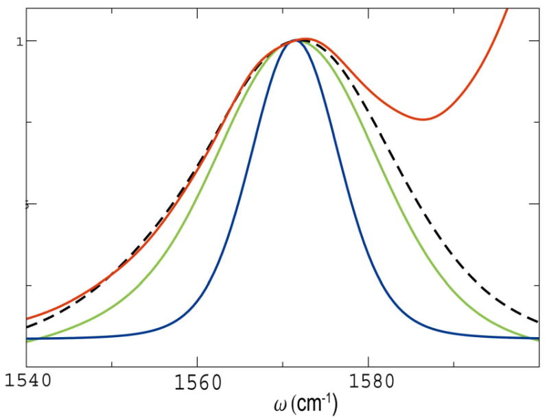
Fig. 6 shows the simulated CGF linear absorption spectra of the amide I band. Neglecting vibrational relaxation (green line), the fwhm is 19cm−1, after adding the Experimental lifetime broadening 450f s [65](red line), the fwhm becomes 30cm−1, which is remarkably close to the experiment(29cm−1).
FIG. 6.
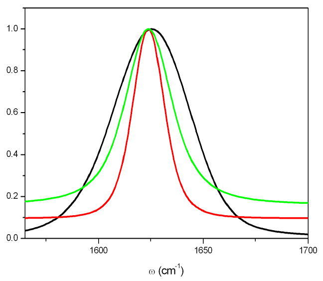
simulated absorption spectra of the amide I band of NMA. CGF, excluding lifetime broadening (green), fwhm (19cm−1), with lifetime broadening (red), the FWHM becomes 30cm−1, which is very close to the experiment(29cm−1)[65]. The inhomogeneous NEE simulated signal (black) overestimates the linewidth (52cm−1)
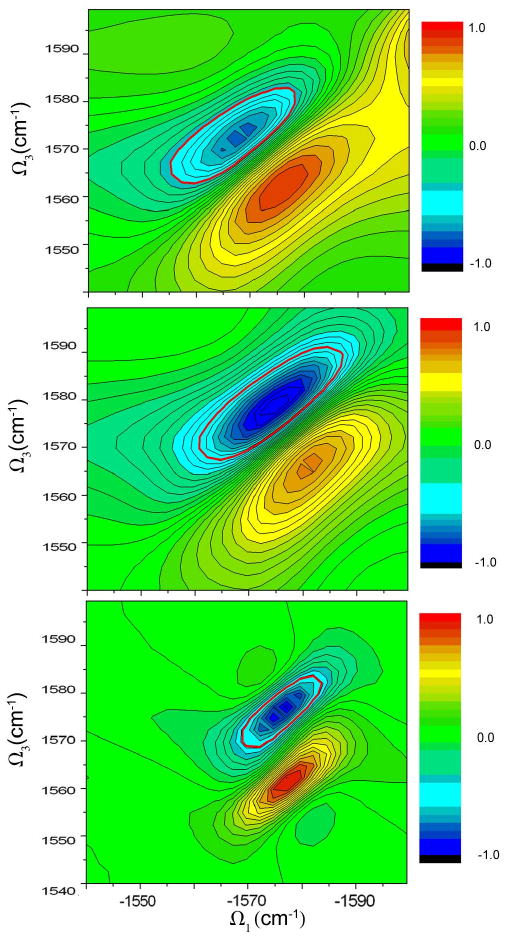
The simulated kI spectra are presented in Fig. 7 both excluding (upper panel) and including (middle panel) vibrational relaxation. The finite vibrational lifetime is significant in this case. For comparison, we have carried out an NEE simulation. Both linear absorption (Fig. 6, black) and the kI signal (Fig. 7, lower panel) are broader than the CGF. The inhomogeneous averaging protocol assumes that the energy fluctuations are much slower than their inverse magnitude. Obviously, this assumption is not justified for NMA where motional narrowing, included in the CGF, should be taken into account.
FIG. 7.
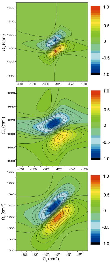
CGF simulated kI spectrum of NMA (imaginary plot) without (top) and with (middle) vibrational relaxation. NEE simulation (bottom)
VIII. The Vibrational Response of YKKKH17
Our MD simulation of the α helical peptide used the velocity verlet algorithm and includes all the atoms of one YKKKH17 molecule and 4330 water molecules. 4 chloride ions were added into the simulation box to make the system neutral. The initial YKKKH17 structure was obtained from the maestro package [69]. The charmm27 force field [44] was employed for all interactions with a cutoff of 12Å for the nonbonded interactions. Long- range electrostatic interactions were calculated using the Ewald Sum [70]. The simulation was carried using the CHARMM package [44]. The structure was first refined in vacuum using a 4000 step energy minimization procedure with Adopted Basis Newton-Raphson method (ABNR)[44]. The molecule was then embedded in a cubic unit cell of TIP3 water with box length of 52Å. To release the internal tension, a 10000 steps Adopted Basis Newton-Raphson energy minimization was performed [44]. The system was equilibrated under NPT ensemble [71] with 1 fs time step for 2 ns to obtain the right system density and box size, the extended system method was used to keep the temperature and pressure constant, and the final box length was 50.19Å. This was followed by an NVE equilibration with 2fs time step for 10ns. After the equilibration phase, a 1 ns trajectory was recorded by applying the NVE ensemble with 1fs time step. The structure was saved in 4 fs increments, giving a total of 2.5 × 10⁵ sample points. The peptide unit (O=C=N-H) is first aligned into the geometry optimized NMA structure of [51]. The fluctuating vibrational Hamiltonian was created for all snapshots along the trajectory. All water molecules were included into the bath.
In the NEE simulations, 100 snapshots with 20 ps time intervals are selected from the 2 ns trajectory and used for the inhomogeneous averaging, (sampling was tested using a 4 ns trajectory which gave very similar inhomogeneous averaged linear absorption). A 5.5 cm−1 homogeneous dephasing rate γ was added[72]. Unlike NMA, the inhomogeneously averaged linear absorption is much broader and is not sensitive to the precise value of γ. The simulated linear absorption is compared with experiment [73] in Fig 8. Both the linewidth and the weak shoulder at 1655 cm−1 are well reproduced.
The bottom panel of Fig 9 gives the distribution of eigenstate energies (density of states). Comparison with the linear absorption spectrum (top) shows that the mid band states have the largest transition dipoles.
FIG. 9.
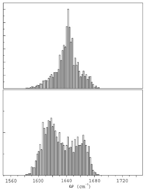
The absorption spectrum (top) and the density of states (bottom) of YKKKH17. Comparing the two panels shows that the mid-band states have the strongest oscillator strength.
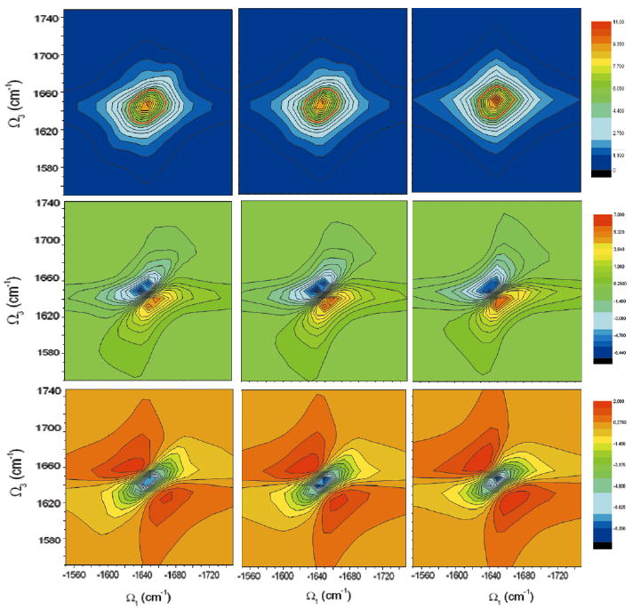
The simulated kI spectrum presented in the left column of Fig. 10 is elongated along the diagonal, this is most clearly seen in the imaginary part (left middle), the diagonal (anti-diagonal) FWHM of the absolute magnitude of the signal (left top) is around 40cm−1 (25cm−1). This is close to the experimental observation in the amide I spectra of a similar 25 residue alpha helical peptide [72]. The simulated kIII spectrum is presented in the right column. Taking as the diagonal line, we obtain ∼ 40cm−1 for the diagonal and “anti-diagonal” width in the amplitude plot (right top). kI is expected to have a smaller anti-diagonal width, since it eliminates some inhomogeneous broadening, this is one major advantage of kI, known as the photon echo. kIII spreads the signal along Ω in a region twice as large as in kI which improves the resolution.
FIG. 10.
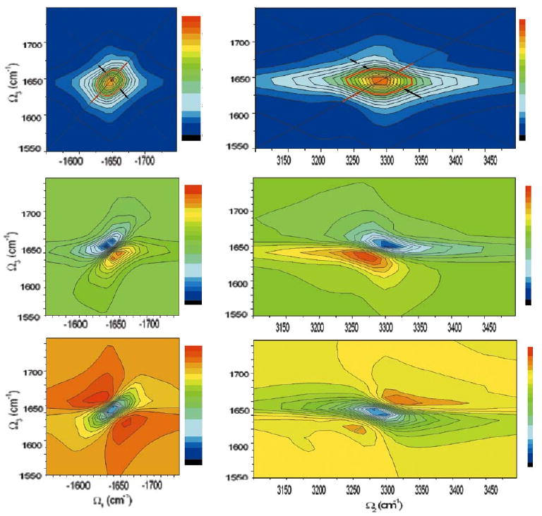
Left column: The NEE simulated kI spectra of YKKKH17 (equation 3): (top) absolute magnitude, The diagonal(solid) and anti-diagonal(dash) line are marked. the half maxima contour is shown(red). Black (Red) arrows mark the diagonal (anti-diagonal) width. (middle) imaginary part and (bottom) real part. Right column repeats these calculations for kIII.
A non-fluctuating experimental anharmonicity -16cm−1 [72] has been assumed in many earlier studies of amide I spectra. To estimate the role of anharmonicity fluctuations, we have calculated the Relative Difference (RD), defined as the difference between the fluctuating anharmonicity and fixed-anharmonicity signals divided by the fixed-anharmonicity signals. The largest RD is 2% for kI and 5% for kIII, indicating that kIII is more sensitive to anharmonicity fluctuations.
Isotopic substitutions are commonly used in the interpretation of vibrational spectra and their relationship to structure[72–74]. Of particular interest to coherent IR applications is the use of isotopes to shift frequencies into regions where the behavior of that local unit can be measured, free from interference with other modes. For the amide I mode, the ∼ −67cm−1 shift by 13C =18 O substitution is large enough to displace the substituted amide group frequencies beyond the range of the natural distribution of frequencies found in most secondary structures. Isolated bands can also be obtained by using other chromophores. For example the nitrile group (C ≡ N) attached to side chains provides a distinct band at ∼ 2235cm−1. It can be used as infrared environmental probes, due to the sensitivity of the CN stretching vibration to hydration as well as other factors [75].
The participation ratio [76] of the exciton state e,
| (28) |
provides a convenient measure for exciton localization which can be used to quantify how much is the isotope band separated from the main band. For a localized exciton We = 1 whereas when e is completely delocalized, and has equal contributions from all the 17 local modes, |Ψem| will equal to and We = 17.
When the first residue is isotopically labelled, We of the lower frequency (1570 cm−1) eigenstates for 1000 configurations has an average value of 1.078 with standard deviation 0.067. |Ψe1|2 has an average value 0.96, with standard deviation 0.003, indicating that the dominant contribution for this state is from the isotopically labelled unit. A similar trend is seen when the 10th residue is isotopically labelled. Fig. 11 shows the isotope region of the inhomogenously averaged simulated linear absorption of the full helix where the first unit is isotopically labelled (red, the isotope peak can be fitted to a Gaussian (black dash) with 28.5cm−1 fwhm), the NEE simulated linear absorption of the labelled mode is given by the green line, with fwhm 26cm−1, the CGF simulated linear absorption of isotope labelled mode (blue, 14.3cm−1). Recent experiment on a similar helical peptide [72] gives a 15.2cm−1 fwhm for the C13O18 labelled peak, in close agreement with the CGF simulation.
FIG. 11.
The isotope region of the NEE simulated linear absorption of the full YKKKH17 helix (red line), the isotope peak fitted to a gaussian (black dash line) with 28.5cm−1 fwhm. The NEE simulated linear absorption of isotope labelled mode (green line, fwhm 26cm−1), The CGF simulated linear absorption of isotope labelled mode (blue line, 14cm−1). The NEE simulated isotope mode reproduces the width and shape of the isotope region of the simulated full helix spectrum. The CGF simulated isotope mode signal is much narrower.
Fig. 12 shows the isotope region of the NEE simulated kI signal of the full helix (top panel) and of the isotopically labelled mode (NEE,middle), (CGF,bottom). Because the isotope band is spectrally isolated, the NEE simulated isotope mode signal mainly reproduces the width and shape of the isotope region of the simulated full helix spectrum, the CGF simulated isotope mode signal is much narrower (motional narrowing).
FIG. 12.
The isotope region of the NEE simulated kI signal (imaginary plot) of the full YKKKH17 helix (upper panel). Simulation of the isotopically labelled mode alone (NEE, middle panel), (CGF, lower panel).)
Isotope labelling also affects the main peak lineshape, in a way that depends on the labelled site. In the upper panel of Fig 13, we show the linear absorption of native, 1st residue labelled (green) and 10th residue labelled (red) helices simulated by NEE. Labelling the 10th residue significantly changes the lineshape while labelling the 1st hardly affected it. This is more clearly demonstrated using the relative difference of linear absorption between isotopomer and unlabelled helix, shown in the lower panel of Fig. 13.
FIG. 13.
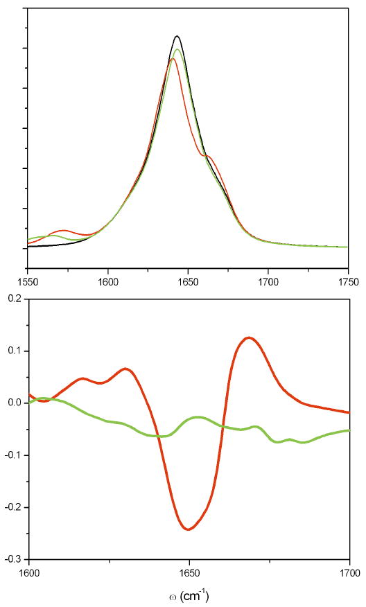
(top) The NEE simulated absorption spectrum of native helix (black), the central 10th residue C13O18 isotope labelled (red) and 1st residue labelled (green) helices. The isotopic effect is simulated by adding a −67cm−1 shift to the local frequency εm(Q) in Eq. (8). (bottom) The Relative Difference of linear absorption signal between isotopomer and native helix. The 10th residue labelled (red) and 1th residue labelled (green). Labelling the central residues has a stronger effect on the lineshape.
IX. Discussion
We have developed first-principles protocols for simulating the coherent infrared spectra of the amide I band of peptides. Two methods, the CGF and NEE, which make different approximations and reproduce a broad range of properties were compared. These are the first attempts to simulate coherent nonlinear signals in large globular proteins.
The NEE approach only uses the one-exciton basis and attributes the nonlinear response to exciton-exciton scattering. Homogeneous broadening is explicitly incorporated in the equations of motion and inhomogeneous contributions are added by ensemble averaging. Classifying the broadening mechanisms either as homogeneous or inhomogeneous is not always possible and does not apply for intermediate fluctuation timescales as required for short peptides. The complete scattering matrix size and the computational effort scales to the fourth power in size. Predicting the dominant scattering configurations (e4e3e2e1) in the scattering matrix based on the exciton overlap parameters η(2) and η(1) leads to a truncation scheme based on the assumption that excitons cannot scatter unless they spatially overlap. This truncation applies for anharmonicities with finite interaction range. It identifies the possible scattering configurations before calculating the scattering matrix itself. The number of scattering configurations and thefore the size of the effective scattering matrix are greatly reduced. Linear scaling of the simulation cost with system size for systems larger than the exciton coherence size makes them particularly attractive for large peptides.
We next illustrate the reduction in computational cost obtained using in equation 26. Fig 14 compares the calculated kI spectrum with all scattering configurations (left), η(1) = 0.3 (middle) and η(1) = 0.5 truncation(right) (we used ). The red circles in the top plot give the half maximum contour. The left spectrum took 35 hours on an AMD Opteron 244 cpu, compared with 2 hours for the middle spectrum. The right spectrum (20 minutes) reproduces the main pattern. The diagonal and anti-diagonal FWHMs obtained from the truncated schemes coincide with the complete scattering matrix, however some of the details are lost. The effect of this favorable scaling should be more dramatic for larger proteins.
FIG. 14.
Simulated NEE kI spectra of YKKKH17 with the full scattering matrix (left), and with a truncated scattering matrix with ηC = 0.3 (middle) and ηC = 0.5(right). Top (absolute magnitude), middle (imaginary part), bottom (real part).
This truncation cannot be applied in SOS calculations which require the complete set of two-exciton states. Multiple interferences between different Liouville space pathways then determine the contributions of the various eigenstates. This is especially important for a weakly anharmonic systems. The nonlinear response of the system of harmonic oscillators vanishes identically. In the NEE this interference is naturally built in whereas in the SOS it is obtained only when all possible contributions are combined. The SOS simulation time including numerical matrix diagonalization scales as ∼ N3 with system size.
Periodic systems (such as J aggregates and molecular crystals) have strict selection rules. A few transition dipoles may be very large and many “dark” states can be eliminated before calculating the signals. This could be used to speed up both NEE and SOS simulation. However, the spectra of disordered proteins have no obvious selection rules; they depend on many contributions with similar transition dipole amplitudes. The CGF which is based on the SOS, describes fluctuations with arbitrary timescales and relies on the adiabatic approximation of energy levels. It is, thus, most suitable for small localized modes such as in isotope substitutions and artificially implemented chromophores such as nitrile groups [75].
Isotope substitutions in vibrational spectroscopy provide an ideal local probe for structure and dynamics. This is conceptually similar to mutations used extensively in studies of biomolecular complexes. By labelling specific sites, isotopes can be used to explore local amide environments and coupling dependence on distances and orientations of amide groups. The CGF is suitable for simulating systems with well-separated energy levels, and reproduces the motional narrowing effect caused by fast fluctuations. Inhomogeneous averaging of slow bath motions can be combined with CGF for intermediate size systems. However, due to its ∼ N3 scaling, this procedure is expensive. A detailed analysis of the linewidths as a function of residue along the helix and the variation of the motional narrowing with the environment will be of interest for a future study.
The zero-order frequencies in our Hamiltonian were obtained from an electrostatic DFT map, which describes the frequency shift of the amide I mode in response to a spatially nonuniform external electric field. This map which allows the simulations of any peptide and solvent neglects covalent interactions of the amide unit with the surrounding molecules. This may account for the lower accuracy of the frequency shift compared with the cluster methods (56 cm−1 vs. ∼ 62cm−1, experimental value is 91 cm−1). Nevertheless the electrostatic fluctuations model seems to adequately reproduce the dominant feautures of the vibrational spectra. We have used a 19 component vector CT to describe the electric field property at one amide unit. This vector is obtained by doing a least square fitting of electric field components of 67 points in the Transition Charge Density region. In a previous work [51], different sampling scheme were tested for the calculation of linear spectra of all amide bands (III, II, I and A) of NMA. For amide I and A stretching motions, CT can be obtained by fitting the electric field at the amide atom positions (C,O,N,H, however the global sampling were found to be crucial for the bending modes (III and II). Overall the global sampling works best.
Lifetime broadening is significant in NMA, however, CGF simulated isotope peaks which neglect lifetime broadening agree with experiment, implying that vibrational relaxation is less important in the vibrational lineshapes of α helical peptides. Predicting the 2DIR signatures of vibrational relaxation and transport behavior of different peptide structures is an interesting open problem. These are expected to show up in the t2 variation of photon echo or pump probe experiments.
The present protocols should help the interpretation of nonlinear vibrational signals from a broad range of biological systems. The vibrational relaxation of N-H stretching in nucleic acids [83–85] is believed to play an important role in the photophysics of DNA and RNA. Time resolved IR spectra can be simulated. Another promising example is carbonhydrates, whose dynamics is faster than the time resolution of NMR but may be studied in the Infrared [86]. One potential application is to amyloid fibrils, which form in Alzheimer's disease and whose structure and dynamics are under extensive study. Recently the fibrils have been crystalized and the structure has been resolved by X-ray [77]. However, the early stage of the fibril formation, during which the randomly coiled or helical peptides collide in the solution, change into hairpins and start to form the oligomers and finally become the fibrils [78–80], is still unresolved. Because of its sensitivity to H-bonding structure, backbone angles and electrostatic environment, multidimensional IR spectroscopy should help resolve this problem. Recent modelling of the kI and kIII spectra of ideal β sheets and helices [64]show that by tuning the pulse polarizations, significant difference can be observed in the kIII spectra between helices and sheets due to differences in local chirality. Time-domain chiral techniques can be used to detect the early dynamics of amyloid fibrils formation.
Most effort in infrared spectroscopy of peptides has so far been focused on the Amide I band and its cross peaks. The cross peak pattern of other amide bands such as amide II and A can provide additional structural information. A DFT map for all amide bands has been constructed [51].
The CGF and NEE approaches were originally developed for electronic spectroscopy [87] and have been used to predict multidimentional electronic spectroscopy in conjugated polymers and photosynthetic aggregates. Electronic spectra are more complex than vibrational spectra and their simulation pose additional challenges. 2D measurements of photosynthetic complexes have been reported [88, 89].
Both CGF and NEE methods hold for equilibrated fluctuations or slow nonequilibrated adiabatic dynamics. For faster fluctuations, the direct simulation involves multiple level crossings and becomes much more expensive. In this case an alternative approach will be to include explicitly the relevant collective bath modes and work in an extended phase space using the stochastic Liouville equations [81, 82].
FIG. 8.
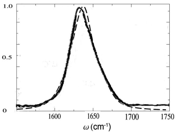
NEE simulated (dash) and experimental [73] (solid) absorption spectrum of YKKKH17. The experimental (simulation) peak position is 1633cm−1 (1643cm−1), fwhm 36cm−1 (36cm−1). The simulated peak was red shifted by 6 cm−1 for a better comparison of the lineshape.
Acknowledgments
This work was supported by the National Institutes of Health Grant 2RO1-GM59230-05 and the National Science Foundation Grant CHE-0446555. We thank Professor Hajime Torii for providing numerical values of the ab initio map of amide I mode couplings. We thank Dr. Ravindra Venkatramani and Dr. Thomas la Cour Jansen for many helpful discussions.
References
- 1.Frauenfelder H, Sligar SG, Wolynes PG. Science. 1991;254(5038):1598–1603. doi: 10.1126/science.1749933. [DOI] [PubMed] [Google Scholar]
- 2.Shakhnovich EI. Current Opinion in Structural Biology. 1997;7(1):29–40. doi: 10.1016/s0959-440x(97)80005-x. [DOI] [PubMed] [Google Scholar]
- 3.Karplus M, McCammon JA. Nature Structural Biology. 2002;9(9):646–652. doi: 10.1038/nsb0902-646. [DOI] [PubMed] [Google Scholar]
- 4.McCammon J, Harvey S. Dynamics of Proteins and Nucleic Acids. Cambridge University Press; Cambridge: 1987. [Google Scholar]
- 5.Onuchic JN, LutheySchulten Z, Wolynes PG. Annual Review of Physical Chemistry. 1997;48:545–600. doi: 10.1146/annurev.physchem.48.1.545. [DOI] [PubMed] [Google Scholar]
- 6.Bryngelson JD, Onuchic JN, Socci ND, Wolynes PG. Proteins-Structure Function and Genetics. 1995;21(3):167–195. doi: 10.1002/prot.340210302. [DOI] [PubMed] [Google Scholar]
- 7.Wolynes PG, Onuchic JN, Thirumalai D. Science. 1995;267(5204):1619–1620. doi: 10.1126/science.7886447. [DOI] [PubMed] [Google Scholar]
- 8.Kubelka J, Hofrichter J, Eaton W. Current Opinion in Structural Biology. 2004;14:76–88. doi: 10.1016/j.sbi.2004.01.013. [DOI] [PubMed] [Google Scholar]
- 9.Ballow R, Sabelko J, Gruebele M. Nat Struct Biol. 1996;3:923. doi: 10.1038/nsb1196-923. [DOI] [PubMed] [Google Scholar]
- 10.williams S, Causgrove T, Gilmanshin R, Fang K, Callender R, Woodruff W, Dyer R. Biochemistry. 1996;35:691. doi: 10.1021/bi952217p. [DOI] [PubMed] [Google Scholar]
- 11.Munoz V, Thompson P, Hofrichter J, Eaton W. Nature. 1997;390:196. doi: 10.1038/36626. [DOI] [PubMed] [Google Scholar]
- 12.werner J, Dyer R, Fesinmeyer R, Andersen N. J Phys Chem B. 2002;106:487. [Google Scholar]
- 13.Huang C, Getahun Z, Zhu Y, Klemke J, DeGrado W, Gai F. Proceedings of the National Academy of Sciences of the United States of America. 2002;99(5):2788. doi: 10.1073/pnas.052700099. [DOI] [PMC free article] [PubMed] [Google Scholar]
- 14.Duan Y, Kollman P. Science. 1998;282:740. doi: 10.1126/science.282.5389.740. [DOI] [PubMed] [Google Scholar]
- 15.Daura X, Jaun B, Seeback D, Van gunsteren WF, Mark A. J Mol Biol. 1998;280:925. doi: 10.1006/jmbi.1998.1885. [DOI] [PubMed] [Google Scholar]
- 16.Zhou Y, Karplus M. Nature. 1999;401:400. doi: 10.1038/43937. [DOI] [PubMed] [Google Scholar]
- 17.Krimm S, Bandekar J. Adv Protein Chem. 1986;38:181. doi: 10.1016/s0065-3233(08)60528-8. [DOI] [PubMed] [Google Scholar]
- 18.Decius WEB, Cross JC. Molecular Vibrations: The Theory of Infrared and Raman Vibrational Spectra. McGraw-Hill; New York: 1955. [Google Scholar]
- 19.Torii H, Tasumi M. J Chem Phys. 1992;96:3379. [Google Scholar]
- 20.Torii H, Tasumi M. J Raman Spec. 1998;29(1):81–86. [Google Scholar]
- 21.Baumruk V, Pancoska P, Keiderling TA. Journal of Molecular Biology. 1996;259(4):774–791. doi: 10.1006/jmbi.1996.0357. [DOI] [PubMed] [Google Scholar]
- 22.Cheatum CM, Tokmakoff A, Knoester J. J Chem Phys. 2004;120:8201. doi: 10.1063/1.1689637. [DOI] [PubMed] [Google Scholar]
- 23.Huang CY, He S, DeGrado WF, McCafferty DG, Gai F. Journal of the American Chemical Society. 2002;124(43):12674–12675. doi: 10.1021/ja028084u. [DOI] [PubMed] [Google Scholar]
- 24.Mantsch HH, Chapman D, editors. Infrared Spectroscopy of Biomolecules. Wiley-Liss; New York: 1996. [Google Scholar]
- 25.Tanimura Y, Mukamel S. Journal of Chemical Physics. 1993;99(12):9496–9511. [Google Scholar]
- 26.Abramavicius D, Zhuang W, Mukamel S. Journal of physical Chemistry B. 2004;108:18034. [Google Scholar]
- 27.Demirdoven N, Cheatum CM, Chung HS, Khalil M, Knoester J, Tokmakoff A. Journal of the American Chemical Society. 2004;126(25):7981–7990. doi: 10.1021/ja049811j. [DOI] [PubMed] [Google Scholar]
- 28.Zhuang W, Abramavicius D, Mukamel S. Proceedings of the National Academy of Sciences of the United States of America. 2005;102(21):7443–7448. doi: 10.1073/pnas.0408781102. [DOI] [PMC free article] [PubMed] [Google Scholar]
- 29.Mukamel S. Annual Review of Physical Chemistry. 2000;51:691–729. doi: 10.1146/annurev.physchem.51.1.691. [DOI] [PubMed] [Google Scholar]
- 30.Bredenbeck J, Helbing J, Behrendt R, Renner C, Moroder L, Wachtveitl J, Hamm P. Journal of Physical Chemistry B. 2003;107(33):8654–8660. [Google Scholar]
- 31.Asplund MC, Zanni MT, Hochstrasser RM. Proceedings of the National Academy of Sciences of the United States of America. 2000;97(15):8219–8224. doi: 10.1073/pnas.140227997. [DOI] [PMC free article] [PubMed] [Google Scholar]
- 32.Golonzka O, Khalil M, Demirdoven N, Tokmakoff A. Physical Review Letters. 2001;86(10):2154–2157. doi: 10.1103/PhysRevLett.86.2154. [DOI] [PubMed] [Google Scholar]
- 33.Larsen O, Bodis P, Buma W, Hannam J, Leigh D, Woutersen S. Proceedings of the National Academy of Sciences of the United States of America (in press) 2005 doi: 10.1073/pnas.0505313102. [DOI] [PMC free article] [PubMed] [Google Scholar]
- 34.Ernst RR, Bodenhausen G, Wokaun A. Principles of nuclear magnetic resonance in one and two dimensions. Oxford University Press; New York: 1995. [Google Scholar]
- 35.Wuthrich K. NMR of Proteins and Nucleic Acids. Wiley-Interscience; 1986. [Google Scholar]
- 36.Henry ER, Szabo A. Journal of chemical physics. 1985;82(11):4753. [Google Scholar]
- 37.Lindorff-Larsen K, Best RB, DePristo MA, Dobson CM, Vendruscolo M. Nature. 2005;433(7022):128–132. doi: 10.1038/nature03199. [DOI] [PubMed] [Google Scholar]
- 38.Tjandra N, Feller S, Paster R, Bax A. Journal of the American Chemical Society. 1995;117:12562–12566. [Google Scholar]
- 39.Scheurer C, Mukamel S. Bulletin of the Chemical Society of Japan. 2002;75(5):989–999. [Google Scholar]
- 40.Scheurer C, Mukamel S. Journal of Chemical Physics. 2002;116(15):6803–6816. [Google Scholar]
- 41.Elber R. Current Opinion in Structural Biology. 2005;15(2):151–156. doi: 10.1016/j.sbi.2005.02.004. [DOI] [PubMed] [Google Scholar]
- 42.Kale L, Skeel R, Bhandarkar M, Brunner R, Gursoy A, Krawetz N, Phillips J, Shinozaki A, Varadarajan K, Schulten K. Journal of Computational Physics. 1999;151(1):283–312. [Google Scholar]
- 43.Van gunsteren WF, Berendsen HJC. Angewandte Chemie. 1990;29(9):992–1023. [Google Scholar]
- 44.Brooks BR, Bruccoleri RE, Olafson BD, States DJ, Swaminathan S, Karplus M. Journal of Computational Chemistry. 1983;4(2):187–217. [Google Scholar]
- 45.Mukamel S, Abramavicius D. Chemical Reviews. 2004;104(4):2073–2098. doi: 10.1021/cr020681b. [DOI] [PubMed] [Google Scholar]
- 46.Fried LE, Mukamel S. Advanced Chemical Physics. 1993;84:435. [Google Scholar]
- 47.Chernyak V, Zhang WM, Mukamel S. J Chem Phys. 1998;109:9587. [Google Scholar]
- 48.Piryatinski A, Chernyak V, Mukamel S. Chem Phys. 2001;266:285. [Google Scholar]
- 49.Mukamel S. In: Molecular Nonlinear Optics. Zyss J, editor. Academic Press; New York: 1994. pp. 1–46. [Google Scholar]
- 50.Mukamel S. Principles of Nonlinear Optical Spectroscopy. Oxford University Press; Oxford: 1995. [Google Scholar]
- 51.Hayashi T, Zhuang W, Mukamel S. Journal of physical chemistry (in print) [Google Scholar]
- 52.Peyerimhoff S. Spectroscopy:Computational Methods, Vol. 1 of Encyclopedia of Computational Chemistry. John Wiley; 1998. [Google Scholar]
- 53.Dreyer J, Moran AM, Mukamel S. Journal of Physical Chemistry B. 2003;107(24):5967–5985. [Google Scholar]
- 54.Kopelman R. In: Excited States. Lim E, editor. Academic; New York: 1975. [Google Scholar]
- 55.Scott AC. Phys Rep. 1992;217:1. [Google Scholar]
- 56.Kwac K, Cho MH. Journal of Chemical Physics. 2003;119(4):2247–2255. [Google Scholar]
- 57.Schmidt JR, Corcelli SA, Skinner JL. Journal of Chemical Physics. 2004;121(18):8887–8896. doi: 10.1063/1.1791632. [DOI] [PubMed] [Google Scholar]
- 58.Kubelka J, Keiderling TA. Journal of Physical Chemistry A. 2001;105(48):10922–10928. [Google Scholar]
- 59.Frisch MJ, et al. Gaussian 03, revision c.01 Technical report. 2003 [Google Scholar]
- 60.Hayashi T, Jansen TL, Zhuang W, Mukamel S. Journal of Physical Chemistry A. 2005;109(1):64–82. doi: 10.1021/jp046685x. [DOI] [PubMed] [Google Scholar]
- 61.Guo H, Karplus M. Journal of Physical Chemistry. 1992;96(18):7273–7287. [Google Scholar]
- 62.Torii H, Tatsumi T, Tasumi M. Journal of Raman Spectroscopy. 1998;29(6):537–546. [Google Scholar]
- 63.Ham S, Kim JH, Lee H, Cho MH. Journal of Chemical Physics. 2003;118(8):3491–3498. [Google Scholar]
- 64.Abramavicius D, Mukamel S. Journal of Chemical Physics. 2005;122(13) doi: 10.1063/1.1869495. [DOI] [PubMed] [Google Scholar]
- 65.Zanni MT, Asplund MC, Hochstrasser RM. J Chem Phys. 2001;114(10):4579–4590. [Google Scholar]
- 66.Mukamel S. Phys Rev A. 1983;28:3480. [Google Scholar]
- 67.Venkatramani R, Mukamel S. Journal of Chemical Physics. 2002;117(24):11089–11101. [Google Scholar]
- 68.Zhang WM, Meier T, Chernyak V, Mukamel S. Journal of Chemical Physics. 1998;108(18):7763–7774. [Google Scholar]
- 69.Mohamadi F, Richards NGJ, Guida WC, Liskamp R, Lipton M, Caufield C, Chang G, Hendrickson T, Still WC. J Comput Chem. 1990;11(4):440–467. [Google Scholar]
- 70.Essmann U, Perera L, Berkowitz ML, Darden T, Lee H, Pedersen LG. Journal of Chemical Physics. 1995;103(19):8577–8593. [Google Scholar]
- 71.Hoover WG. Physical Review A. 1985;31(3):1695–1697. doi: 10.1103/physreva.31.1695. [DOI] [PubMed] [Google Scholar]
- 72.Fang C, Wang J, Kim YS, Charnley AK, Barber-Armstrong W, Smith AB, Decatur SM, Hochstrasser RM. Journal of Physical Chemistry B. 2004;108(29):10415–10427. [Google Scholar]
- 73.Decatur SM, Antonic J. Journal of the American Chemical Society. 1999;121:11914–11915. [Google Scholar]
- 74.Moran AM, Park SM, Dreyer J, Mukamel S. J Chem Phys. 2003;118(8):3651–3659. [Google Scholar]
- 75.Tucker MJ, Getahun Z, Nanda V, DeGrado WF, Gai F. Journal of the American Chemical Society. 2004;126(16):5078–5079. doi: 10.1021/ja032015d. [DOI] [PubMed] [Google Scholar]
- 76.Thouless D. Phys Rep. 1974;13:93. [Google Scholar]
- 77.Ritter C, Maddelein ML, Siemer AB, Luhrs T, Ernst M, Meier BH, Saupe SJ, Riek R. Nature. 2005;435(7043):844–848. doi: 10.1038/nature03793. [DOI] [PMC free article] [PubMed] [Google Scholar]
- 78.Kirschner DA, Inouye H, Duffy LK, Sinclair A, Lind M, Selkoe DJ. Proceedings of the National Academy of Sciences of the United States of America. 1987;84(19):6953–6957. doi: 10.1073/pnas.84.19.6953. [DOI] [PMC free article] [PubMed] [Google Scholar]
- 79.Inouye H, Fraser PE, Kirschner DA. Biophysical Journal. 1993;64(2):502–519. doi: 10.1016/S0006-3495(93)81393-6. [DOI] [PMC free article] [PubMed] [Google Scholar]
- 80.Serpell LC, Blake CCF, Fraser PE. Biochemistry. 2000;39(43):13269–13275. doi: 10.1021/bi000637v. [DOI] [PubMed] [Google Scholar]
- 81.Jansen TlC, Zhuang W, Mukamel S. J Chem Phys. 2004;121:10577–10598. doi: 10.1063/1.1807824. [DOI] [PubMed] [Google Scholar]
- 82.Gamliel D, Levanon H. Stochastic Processes in Magnetic Resonance. World Scientific; River Edge,NJ: 1995. [Google Scholar]
- 83.Woutersen S, Cristalli G. Journal of Chemical Physics. 2004;121(11):5381–5386. doi: 10.1063/1.1785153. [DOI] [PubMed] [Google Scholar]
- 84.Kyogoku Y, Lord RC, Rich A. Science. 1966;154(3748):518–532. [PubMed] [Google Scholar]
- 85.Hamlin RM, Lord RC, Rich A. Science. 1965;148(3678):1734–1748. doi: 10.1126/science.148.3678.1734. [DOI] [PubMed] [Google Scholar]
- 86.Liquier J, Letellier R, Dagneaux C, Ouali M, Morvan F, Raynier B, Imbach JL, Taillandier E. Biochemistry. 1993;32(40):10591–10598. doi: 10.1021/bi00091a008. [DOI] [PubMed] [Google Scholar]
- 87.Chernyak V, Wang N, Mukamel S. Phys Rep. 1995;263:213–309. [Google Scholar]
- 88.Brixner T, Stenger J, Vaswani HM, Cho M, Blankenship RE, Fleming GR. Nature. 2005;434(7033):625–628. doi: 10.1038/nature03429. [DOI] [PubMed] [Google Scholar]
- 89.Sundstrom V, Pullerits T, van Grondelle R. Journal of Physical Chemistry B. 1999;103(13):2327–2346. [Google Scholar]