mGene: Accurate SVM-based gene finding with an application to nematode genomes

Abstract

We present a highly accurate gene-prediction system for eukaryotic genomes, called mGene. It combines in an unprecedented manner the flexibility of generalized hidden Markov models (gHMMs) with the predictive power of modern machine learning methods, such as Support Vector Machines (SVMs). Its excellent performance was proved in an objective competition based on the genome of the nematode Caenorhabditis elegans. Considering the average of sensitivity and specificity, the developmental version of mGene exhibited the best prediction performance on nucleotide, exon, and transcript level for ab initio and multiple-genome gene-prediction tasks. The fully developed version shows superior performance in 10 out of 12 evaluation criteria compared with the other participating gene finders, including Fgenesh++ and Augustus. An in-depth analysis of mGene's genome-wide predictions revealed that ≈2200 predicted genes were not contained in the current genome annotation. Testing a subset of 57 of these genes by RT-PCR and sequencing, we confirmed expression for 24 (42%) of them. mGene missed 300 annotated genes, out of which 205 were unconfirmed. RT-PCR testing of 24 of these genes resulted in a success rate of merely 8%. These findings suggest that even the gene catalog of a well-studied organism such as C. elegans can be substantially improved by mGene's predictions. We also provide gene predictions for the four nematodes C. briggsae, C. brenneri, C. japonica, and C. remanei. Comparing the resulting proteomes among these organisms and to the known protein universe, we identified many species-specific gene inventions. In a quality assessment of several available annotations for these genomes, we find that mGene's predictions are most accurate.

A decade ago, an 8-yr-long collaborative effort resulted in the first completely sequenced genome of a multicellular organism, the nematode Caenorhabditis elegans (The C. elegans Sequencing Consortium 1998). Today, next-generation technologies have rendered genome sequencing an almost routine process, allowing individual scientists to obtain the sequences of their favorite organisms. The task of annotating new genomes may therefore move partly into the domain of individual researchers or laboratories. Consequently, labor-intense procedures like manual annotation by experts, albeit presumably most precise, are not always affordable, and highly automated computational methods are called upon to fill the gap.

Recently, computational gene finding has experienced a major breakthrough by adopting discriminative machine learning techniques (Brent 2008). In contrast to generative gene-finding methods, which jointly model the DNA sequence itself together with its segmentation into gene structures, discriminative techniques only attempt to find the most accurate gene segmentation for a given DNA sequence.9 On sequence-labeling tasks in natural language processing, as well as genome annotation, discriminative strategies have been shown to outperform generative hidden Markov models (HMMs) (Tsochantaridis et al. 2004; DeCaprio et al. 2007). As one of the first groups to reap this benefit for gene finding, we developed mSplicer, which accurately predicts the exon–intron structure given the unspliced mRNA (Rätsch and Sonnenburg 2007; Rätsch et al. 2007). In this work we present mGene, which is a complete discriminative gene finder conceptually similar to mSplicer. Its strength has been demonstrated in a fair and independent competition for nematode genome annotation (nGASP) (Coghlan et al. 2008), where it exhibited an excellent performance compared with 47 submitted predictions from 17 research groups, including Fgenesh (Salamov and Solovyev 2000), Augustus (Stanke et al. 2006), Craig (Bernal et al. 2007), and N-Scan (Gross and Brent 2006). mGene's superior ab initio performance on nucleotide, exon, and transcript levels can be attributed to a combination of design choices, most importantly: (1) its comprehensive, biologically accurate gene model, (2) the utilization of very precise submodels to recognize genic features (sites and regions), and (3) the integration of the resulting feature scores by means of discriminative methods:

1. The basis of most gene finders is to recognize splice sites, translation initiation sites (TIS), and translation termination sites (Stop). mGene surpasses other gene finders in that it explicitly models a more comprehensive list of signal sites. First, mGene includes transcription start and stop sites, and can thus predict untranslated regions (UTRs). Besides constituting valuable biological information in themselves, correctly predicted UTRs are also expected to improve the overall accuracy for protein-coding genes (Brown et al. 2005). For the same reasons, we also incorporated polyadenylation (poly(A) sites, which are known to be rather strong signals at the end of genes) (Liu et al. 2003). As an additional extension, 5′ UTRs and 3′ UTRs are allowed to be spliced in our model. Optionally, mGene's model also represents trans-splicing and operons, which are especially relevant to nematodes (Graber et al. 2007).

2. It is essential for gene finders to detect functional DNA sequence features, such as transcription start sites (TSS) or splice sites, with the highest possible precision. In earlier work we have shown that support vector machines (SVMs) (cf. Schölkopf and Smola 2002) with certain higher-order DNA sequence kernels yield the most accurate translation start, transcription start, and splice-site recognition (Zien et al. 2000; Sonnenburg et al. 2006, 2007b; Ben-Hur et al. 2008). We devised such signal detectors for all modeled signals. Further, content detectors are used to distinguish different types of segments (e.g., exon or intron) by their typical composition of substrings. Again, high accuracy is achieved by training SVM models utilizing high-order dependencies of nucleotides on large training data sets. To be able to use these SVMs in mGene, we have decoupled the feature recognition tasks from the gene structure prediction problem and treated them as independent binary classification tasks. This allows us to take advantage of millions of available training examples to improve the recognition accuracy (Sonnenburg et al. 2007a,b).

3. The detector scores computed by SVMs are combined to form a globally plausible gene structure. Here, we use hidden semi-Markov SVMs (HSM–SVMs) (Rätsch and Sonnenburg 2007), a discriminative learning technique to predict structured outputs (see also Tsochantaridis et al. 2005). In contrast to generative models like HMMs, discriminative approaches do not model the complex processes that generated the DNA sequence, and thereby avoid many potential modeling mistakes. Like generalized HMMs (gHMMs) (Stormo and Haussler 1994), HSM–SVMs have semi-Markovian properties, which allow mGene to utilize the length distributions of the different segment types.

From a technical perspective, mGene is closely related to recently proposed discriminative gene-finding systems such as Craig (Bernal et al. 2007), Conrad (DeCaprio et al. 2007), and Contrast (Gross et al. 2007). How these approaches conceptually compare with mGene will be examined in the Discussion section.

Results

Performance evaluation on nGASP data

One of the major difficulties in research on new computational methods in general is to assess their accuracy in comparison to previously published ones with as little bias as possible. This is particularly true for gene finders, since even the very definition of a gene is still under discussion (Gerstein et al. 2007). Even subtle differences in evaluation routines may result in substantial differences in the outcome of a comparison. Finally, standardized data sets for training and evaluation are often lacking. Controlled genome annotation assessment projects (Reese et al. 2000; Guigó et al. 2006; Coghlan et al. 2008) are therefore greatly welcome occasions for objective evaluations and comparisons of contemporary state-of-the-art methods. Moreover, the results and protocols of such competitions are often used as a reference in comparisons of improved or newly proposed systems with previous submissions (e.g., Bernal et al. 2007; Gross et al. 2007).

With mGene, we participated in the nematode genome annotation assessment project (nGASP) (Coghlan et al. 2008). The organizers created strictly controlled conditions, precisely specifying any data that was allowed to be used (details are available from the competition website and in the Supplemental information). The performance metrics used were similar to those used in the EGASP competition (Guigó et al. 2006): Sensitivity and specificity were determined on the level of nucleotides, exons, transcripts, and genes, while considering coding regions only. In the nGASP competition a set of highly confirmed genes was used for sensitivity assessment, while specificity was determined on a broader set.

Four categories were distinguished within the competition (Coghlan et al. 2008):

• Category 1—ab initio predictions, allowing only the genomic sequence as input;

• Category 2—predictions that utilize conservation information from multiple nematode genome alignments;

• Category 3—predictions that make use of alignments of proteins, ESTs, and cDNA sequences to the genome; and

• Category 4—combiners, which benefit from all available information including predictions submitted for categories 1–3.

We participated in categories 1–3 with developmental versions of mGene, which we call mGene.init (dev), mGene.multi (dev), and mGene.seq (dev), respectively. Since the nGASP competition, we have continued to refine mGene and have used it to obtain predictions according to the rules in categories 1 and 3 (denoted by mGene.init and mGene.seq). The results of the nGASP comparison together with the performances of the improved system are summarized in Table 1. Shown are the top performing methods only, which makes differences in prediction accuracy appear small. However, when all participating methods are compared, performance margins can reach 20 percentage points on the gene level (e.g., when comparing mGene.init [dev] to SNAP) (Korf 2004).

Table 1.

Comparison of top performing gene finding systems that participated in the nGASP challenge (Coghlan et al. 2008)

Shown are sensitivity (Sn), specificity (Sp), and their average (each in percent) on nucleotide, exon, transcript, and gene level in categories 1–3 (if several submissions were made for one method, we chose the version with the best gene level average of sensitivity and specificity). The predictions of mGene.init and mGene.seq were generated after the deadline but according to the rules of the nGASP challenge. The result of the best performing method within a category and according to each of the evaluation levels is set in boldface. For reference we also provide the results of the evaluation by the nGASP team (Coghlan et al. 2008) in Supplemental Table SI. The numbers slightly deviate on the transcript and gene level due to minor differences in the evaluation criteria. These differences, however, do not change the ranking except in two cases, where the performances are very close together (relevant results are marked with an asterisk).

The results in Coghlan et al. (2008) show mGene.init (dev) to be more specific than all competing methods (including Fgenesh, Augustus, and Craig) in category 1 (ab initio) on all four levels (see also Fig. 1; Supplemental Fig. SI). The second most specific gene finder was Craig, which had significantly lower sensitivity than mGene. Fgenesh and Augustus achieved higher sensitivity, albeit at the cost of lower specificity. With respect to the average of sensitivity and specificity, mGene.init (dev) was the best among all category 1 submissions on all levels except for the gene level, where it was second to Augustus.

Figure 1.

Improvement of mGene.init ab initio predictions on several evaluation levels: (A) nucleotide, (B) exon, (C) transcript, and (D) gene (each restricted to coding regions), as well as on selected signals: (E) acceptor splice sites, (F) donor splice sites, (G) TIS, (H) translation termination sites, (I) transcription start sites (TSS) (±20 nt), and (J) cleavage sites (±20 nt). mGene.init's predictions are compared with the predictions of the best submissions in category 1: Craig, Eugene, Fgenesh, and Augustus. Shown are differences of percent values for sensitivity (Sn; blue), specificity (Sp; green), and their average (red). Note that Craig and Fgenesh are not able to predict UTRs. We therefore used the predicted translation start and stop as an estimate of gene start and stop (relevant results are marked with an asterisk).

The fully developed version mGene.init now makes predictions that are more accurate than any competing submission to nGASP in category 1. Figure 1, A–D, illustrates the improvements in sensitivity and specificity of mGene.init compared with the best submissions in category 1. Note that these improvements correspond to substantial reductions of the error rate (defined as 1 − ) relative to the second best methods (in parentheses) on each level, namely, 8.9% for nucleotides (Craig), 13.4% for exons (Fgenesh), 8.7% for transcripts (Augustus), and 4.1% for genes (Augustus).

In category 2, mGene.multi (dev) outperformed all competing methods including N-Scan and Eugene (Foissac and Schiex 2005) for all evaluation criteria. It is noteworthy that despite the use of additional information, Eugene and N-Scan were not able to achieve the performance of the best ab initio gene finders. Only mGene.multi (dev) managed to improve slightly over the best methods in category 1. One reason for this unexpected finding may be suboptimal evolutionary distances between C. elegans and the aligned genomes (C. briggsae and C. remanei). Importantly, this reflects the need for accurate ab initio gene finders for genomes lacking deep alignments to other genomes.

For predictions submitted in category 3, the development version mGene.seq (dev) only utilized EST and cDNA alignments, but not the provided protein sequences. Nevertheless, among the seven competitors in this category, only Augustus and Fgenesh were able to achieve higher accuracy (defined as average of sensitivity and specificity) than mGene.seq (dev). The current prediction system, called mGene.seq, exploits EST, cDNA, and protein sequence alignments to improve gene predictions, which are now most accurate according to the evaluation on exon and gene level—only second to Fgenesh on the transcript level.

In addition to the global evaluation of predicted gene structures, it is also interesting to compare prediction systems with respect to individual sequence signals, like transcription/translation start/stop sites, as well as splice sites. We performed such comparisons on the ab initio systems as an indirect assessment of the underlying sequence features. Figure 1, E–J, shows the improvement of mGene's gene predictions relative to the top nGASP submissions: We achieved significantly higher accuracy on all signals except for the cleavage site, where Augustus predictions were found to be more accurate. A detailed evaluation of the signal predictions can be found in Supplemental Section A.2.

Genome-wide predictions for C. elegans and discovery of novel genes

After the evaluation of the competition, the nGASP consortium was provided with genome-wide predictions by the most accurate gene finders, namely mGene.seq, Augustus, Fgenesh++, and subsequently also used the combining system Jigsaw (Allen et al. 2006) as a reconciliation method (Coghlan et al. 2008). The mGene predictions are available on the project website and are displayed in the WormBase genome browser. Additionally, we provide the predictions of individual signal sites for two popular genome browsers (WormBase and UCSC), which may help human curators to annotate genes in the future.

In Table 2 we present a short summary of the main differences between the C. elegans annotation WS180 and the gene predictions by the methods under consideration (more details can be found in Supplemental Table S4). The basic characteristics (mean number of exons per gene, median lengths of exons, introns, and open reading frames [ORFs]) between the catalogs are fairly similar, with Jigsaw being the closest to the annotation and Fgenesh++ the most different. We observe that Fgenesh++ predicts about 9% more genes, but about 10% fewer exons per gene and 8% shorter ORFs than mGene.seq or other gene finders. One possible explanation is that Fgenesh++ splits sequences of exons more often into separate genes than other gene finders. An alternative plausible explanation is that most additionally predicted genes have very few exons (cf. Supplemental Section B). Additionally, we observe that the gene-finding systems detect between 970 (Jigsaw) and 2988 (Fgenesh++) new genes, i.e., genes not present in WS180, while missing between 217 (Fgenesh++) and 822 (Jigsaw) annotated genes. This is consistent with the low sensitivity and high specificity of Jigsaw, and vice versa for Fgenesh++. A majority of the new genes predicted by the combiner Jigsaw were also found by the other three gene-finding systems (82%). mGene missed the fewest confirmed genes, namely only 0.7% of all confirmed genes. Of its predicted genes, 809 are neither present in the annotation nor found by any other gene finder. As we show below, there is good reason to believe that many of them are genuine.

Table 2.

Comparison of the predictions of mGene.seq, Fgenesh++, Augustus, and Jigsaw to the C. elegans genome annotation WS180

The first five columns exhibit relatively small differences with respect to basic gene characteristics. Interestingly, all gene finders predict many genes which are new, i.e., that show no overlap with a coding sequence from WS180; additionally, many new genes are unique to the given gene finder, i.e., they do not overlap with any other prediction. We further report the number of missed genes, i.e., annotated coding sequences that have no predicted counterpart, and among those, the fully EST/cDNA confirmed ones.

In total, 11,393 transcripts from the WS180 annotation (i.e., 48%) completely agreed with a transcript predicted by mGene. The proportion of confirmed annotated transcripts that were correctly predicted is significantly higher (5343/8126, 66%), corresponding well to the reported transcript level sensitivity on the nGASP test regions. Annotated transcripts from completely unconfirmed genes agreed to a considerable lesser extent with mGene's predictions (1209/4657, 26%). mGene predicted 2197 novel genes that are not part of the WS180 annotation. We could associate 621 (28.3%) of these with InterPro domains. Among those, the seven trans-membrane chemoreceptors (103 genes) constitute the largest addition (see Supplemental Section B.2 for further information). Out of the 297 genes in WS180 missed by mGene, we could only associate 27 (9.1%) with InterPro domains. Intriguingly, 1855 novel genes show significant protein sequence similarity to mGene gene predictions in other Caenorhabditis species (see next section).

We then wished to know the fraction of the newly predicted and missed unconfirmed genes for which experimental evidence of gene expression could be found. We conducted a set of validation experiments based on RT-PCR and sequencing of mRNA fragments of selected genes. Following the approach by Siepel et al. (2007), we considered 57 spliced novel genes that were predicted by mGene.seq that do not overlap with an annotated protein-coding gene in WS180. In a second experiment, we selected 24 spliced, unconfirmed protein-coding genes annotated in WS180 that did not overlap with an mGene.seq prediction. If a sequenced fragment could be mapped unambiguously to the genomic region of the corresponding gene, we considered the expression of the gene as experimentally validated. A summary of the experimental validation is given in Table 3. We can observe that a significantly larger fraction of novel genes can be validated as compared with unconfirmed genes missed by mGene.seq and also to previous validation studies in human (Guigó et al. 2006). In summary, both experimental and in silico analyses indicate that a large fraction of newly predicted genes are expressed or even functional, demonstrating that even the gene catalog of a well-studied organism like C. elegans can be substantially improved with mGene predictions.

Table 3.

Experimental analysis of the difference between the C. elegans annotation WS180 and mGene.seq predictions

Shown are the number of new genes and unconfirmed genes missed by mGene.seq relative to WS180, the number of genes considered in validation experiments, and the number and fraction of such genes that were verified to have mRNA expression.

Genome-wide predictions for other nematode genomes

We used the trained system mGene.seq to annotate four other Caenorhabditis genomes that have recently been sequenced (www.genome.wustl.edu; R Wilson, pers. comm.): C. briggsae (assembly cb3), C. brenneri (assembly 4.0), C. remanei (assembly 15.0.1), and C. japonica (assembly 3.0.2) (Stein et al. 2003; Sternberg et al. 2003). The characteristics of the predicted gene catalogs show large differences, as detailed in Supplemental Table S5. To assess the quality of the predictions, we aligned EST sequences from the four nematodes, obtained from the NCBI Nucleotide database, against their respective genomes using BLAT (Kent 2002). We examined the agreement of the predictions of the four gene-finding methods mGene.seq, Fgenesh, Augustus, and Jigsaw with internal exons of the aligned EST sequences. While this approach may not be unbiased (in category 3 the same type of information is actually used to generate predictions), there does not appear to be an alternative in the absence of an independent high-quality annotation. The results of the comparison are given in Figure 2B. We observe that mGene.seq maintains a relatively high exon level accuracy of 93%–97% for all organisms, except for C. briggsae (87%), for which the exon level accuracy is consistently lower across all gene-finding systems. We find that mGene outperforms all other gene-finding systems for all organisms, assuring that the model trained using data from C. elegans is general enough to yield accurate predictions on related genomes. We also observe that for organisms for which initially no or few EST sequences have been available (for instance C. japonica), mGene can still yield strong performance (cf. Supplemental Table S7).

Figure 2.

Comparison of the gene sets predicted by mGene.seq for different nematodes. (A) Number of protein-coding genes predicted for each organism and the fraction of genes with one-to-one orthologs, other orthologs with weak, and with no significant protein sequence similarity. (B) Agreement of internal exons inferred from aligned EST sequences with exons predicted by mGene.seq, Fgenesh++, Augustus, and Jigsaw. We counted a predicted exon as correct if both boundaries were correct, and as a false prediction if it overlapped a region covered by an EST alignment but did not exactly match an EST-confirmed exon. Shown is the average of sensitivity and specificity. (C) Number of orthologous groups (9885) shared among all five nematodes, as well as the number of additional orthologous groups shared across subtrees of more closely related species, which are defined by the corresponding ancestral node.

We carried out a comparative analysis with Multiparanoid (Alexeyenko et al. 2006) on the newly predicted proteomes of C. briggsae (22,542 predictions), C. brenneri (41,129), C. remanei (31,503), and C. japonica (20,121). This analysis served two purposes: first, to determine gene homology relations, and second, to estimate the number of species-specific gene creations. We could identify orthology relations for a proportion of 63%–84% of a species' gene set, with C. brenneri being at the bottom and C. elegans at the top of the list (see Fig. 2; Supplemental Table S8). Substantial sequence similarity (≥50 bits) was found for a proportion of 82%–94% of the predicted protein sets, with C. japonica ranking lowest. These numbers demonstrate that the vast majority of predicted proteins have a phylogenetic counterpart in at least one other species. The genome of C. japonica, which is most distant from any of the other genomes (Kiontke and Sudhaus 2006), shows the greatest proportion of potentially species-specific genes (≥18%). We followed up on the potential function of species-specific genes by comparing them to the known protein universe as defined by the Uniref90 database (Wu et al. 2006) and the recently sequenced satellite nematode, Pristionchus pacificus (Dieterich et al. 2008). Out of the species-specific gene predictions for C. remanei, C. japonica, and C. brenneri, only a very small fraction matched to entries in the Uniref90 database (cf. Supplemental Section C.2). Nevertheless, there are some remarkable exceptions. For instance, we found 90 C. remanei gene predictions that show substantial similarity to bacterial genes from the genus Acinetobacter (soil bacteria) (Gerischer 2008). These predictions contain introns, which argues against bacterial sequence contamination. Among the species-specific gene predictions for C. elegans, there are 341 (31.2%) novel genes. Furthermore, among all novel gene predictions, only 51 match to the Uniref90 database. Hence, the novel genes are highly enriched in the set of unknown genes, which suggests that they are genuinely novel (although we cannot exclude that some of these are false-positive predictions). Generally, we observe no similarity to P. pacificus gene predictions, which is in agreement with the phylogenetic position of P. pacificus as an outgroup. This further supports our interpretation of these Caenorhabditis predictions being species-specific gene inventions.

Discussion

Despite vast technological and scientific advancements, we are still not in possession of a single complete and precise gene catalog for any multicellular organism. This stresses the necessity for progress in computational gene finding, but also presents an obstacle to it because it impedes the assessment of concepts and implementations. It is therefore the great benefit of competitions like nGASP to provide controlled conditions for fair comparisons of the intrinsic potential of different systems. It was in such a setting that mGene's excellent performance was demonstrated. Further improvements have consolidated mGene as one of the most accurate gene finders available, even though since the nGASP competition, other gene-finding systems might have improved as well.10

The runners-up in the ab initio category, Augustus and Fgenesh, both use generative training algorithms and have earlier been shown to perform well on human and fly genomes. In particular, Augustus was one of the best-performing methods in the ab initio category of the human annotation competition EGASP (Guigó et al. 2006). In nGASP, the only other participating discriminative gene finder, Craig, did not perform as well, despite the fact that it was reported to outperform Augustus on a human data set (Bernal et al. 2007). The relatively weak performance of Craig may indicate the importance of good feature models for accurate gene prediction: With Craig, Bernal et al. (2007) attempted to tackle the gene-finding problem in a single step, simultaneously learning local feature properties and global characteristics of gene structures through an integrated training procedure. While this approach is conceptually appealing, it is very demanding in terms of computational resources for state-of-the-art discriminative learning algorithms. It thus prohibits simultaneous use of high-order signal detectors and large amounts of training data, as was done in training mGene. The evaluation corroborates the notion that the disadvantage of simpler signal detectors is not fully compensated for by Craig's global parameter optimization strategy.

Recently, two other discriminatively trained methods, Conrad (DeCaprio et al. 2007) and Contrast (Gross et al. 2007), were published. Both have a two-layered architecture similar to mGene and its predecessor mSplicer (Rätsch et al. 2007). They yielded very promising results on human and fungal genomes. Unfortunately, they did not participate in the nGASP competition, and a direct empirical comparison is therefore pending. However, there are substantial differences in terms of (1) the underlying model, (2) the employed feature scores, and (3) the training algorithm: (1) Among the discriminative gene finders, mGene is the only one that is capable of predicting UTRs, trans-splicing, and polyadenylation sites. (2) For the feature detectors, we use SVMs with one or more high-order DNA sequence kernels (up to order 22) on large sequence windows (up to l000 bp) to obtain the most accurate models for segment boundary detection. In contrast, Conrad only uses position weight matrices (PWMs; corresponding to order 1) for signal detection, which have been shown to be suboptimal on such tasks (Sonnenburg et al. 2006, 2007b). Contrast exploits DNA sequence features within very small windows (6–30 bp) with SVMs and simple quadratic kernels considering second order relations. Well-designed features describing multiple genome alignments, a strength of Conrad and Contrast in many applications, appear to be less crucial for nematode gene predictions. (3) The integrative step in Contrast is based on a standard conditional random field (CRF) framework that does not allow semi-Markov dependencies between labels. Consequently, Contrast is unable to model segment lengths appropriately. Explicit incorporation of length features constitutes an improvement of mGene that is comparable to the advantage of gHMMs over standard HMMs (Burge and Karlin 1998). While mGene uses HSM–SVMs, Conrad is based on semi-Markov CRFs (Sarawagi and Cohen 2004). Both approaches are state-of-the-art structured output prediction techniques. Although the optimization problems solved in the training step differ, their prediction accuracy has often been found to be similar when compared with the same data, with the same underlying model (Keerthi and Sundararajan 2007). It remains to be investigated how the two learning techniques compare for gene finding when identical features are used.

Due to its discriminative framework and the two-layered architecture, mGene is a very flexible system. One advantage of this is that separate data sets can be used for training its individual parts (e.g., the signal detectors). In contrast to less modular systems, it can thus exploit the available data to a fuller extent. As another benefit, mGene's architecture readily allows the integration of additional information from diverse data sources. In the context of nGASP, we implemented first versions of mGene that utilize sequence conservation or known transcript sequences. Although mGene outperforms its competitors in both corresponding categories, these versions may not yet fully exhaust the potential of the input information sources: For instance, the more sophisticated features describing multiple alignments used in Contrast and Conrad may help to further improve mGene's performance. It also appears promising to include additional features such as epigenomic data or transcriptome reads from next-generation sequencing.

From a biological perspective, the nGASP competition serves as a case study of the value of sampling genomes across one genus. Whole-genome assemblies (coverage greater than or equal to sixfold) of five Caenorhabditis species were made available to nGASP participants. Our gene finder mGene, which was just trained on the reference species C. elegans, could exploit the conservation of genic DNA signals to accurately annotate the remaining genomes. This is remarkable if contrasted with the average protein sequence conservation, which is just 78% for the most distant species pair (C. briggsae and C. japonica). Consequently, mGene facilitates whole-genome annotation for related species, even though they diverged from their last common ancestor more than 100 Mya (Stein et al. 2003). In summary, several other comparative sequencing efforts (e.g., in flies and vertebrates) may benefit from using mGene as one of the primary gene-prediction tools.

To make mGene more widely available to the genome annotation community we have developed a webserver, mGene.web at http://mgene.org, which delivers the functionality to predict genes on small to moderately sized eukaryotic genomes using pretrained models for an increasing number of organisms (Schweikert et al. 2009). Additionally, one can easily train new models based on uploaded genomes and preliminary annotations. This webserver will also serve as a convenient platform for future advancements, such as the exploitation of additional sources of evidence, the prediction of alternative transcript variants, and the broader applicability of the system to larger genomes.

Methods

We take a two-layer approach to gene finding (Rätsch et al. 2007). The first layer consists of independent SVM-based signal and content detectors (Sonnenburg et al. 2006, 2007a,b; Rätsch et al. 2007). In the second layer an HSM–SVM (Rätsch and Sonnenburg 2007) combines the scores of the individual detectors together with segment length information to form a valid gene prediction (cf. Fig. 3). We will first describe the ab initio algorithm mGene.init and subsequently outline the extensions for mGene.multi and mGene.seq.

Figure 3.

In layer 1, mGene scans the genomic sequence using SVM-based detectors trained to recognize transcription start sites (TSS), translation initiation sites (TIS), acceptor (Ace), and donor (Don) splice sites, the translation termination site (Stop), and other signals (data not shown). The detectors assign a score to each candidate site. In combination with additional information, including outputs of SVMs recognizing exon/intron content, and scores for exon/intron lengths (data not shown), these signal scores contribute to the cumulative score of a putative gene structure. The bottom graph (layer 2) illustrates the accumulation of scores for two gene structures shown at the top, where the score at the end of the sequence is the final score of the gene structure. The contributions from the individual detector outputs, from segment lengths, as well as from properties of the segments to the score are adjusted during training using piecewise linear functions (PLiFs; see inset to the right). They are optimized such that the margin between the true gene structure (shown in green) and all other (false) isoforms (one of them is shown in red) is maximized. Prediction of genes on new sequences works by selecting a valid gene structure, as defined by the gene model (cf. inset to the left), with the maximum cumulative score using dynamic programming (see e.g., Kulp et al. 1996).

Layer 1: Feature recognition

The core features of our algorithm fall into three distinct classes: sequence signals (at segment boundaries), sequence content (the sequence composition of a given segment), and the lengths of the individual segments. To recognize signals and segment types, we developed detectors that compute corresponding scores. Here, we utilize SVMs with string kernels (for review, see Ben-Hur et al. 2008), because they have been shown to perform with superior accuracy compared with generative methods (like phylogenetic generalized HMMs), for instance, for splice-site detection and TSS (Sonnenburg et al. 2006, 2007b). The real-valued scores that SVMs compute are nonprobabilistic, which makes it difficult to use them in a generative (and thus probabilistic) framework like gHMMs; however, corresponding requirements are absent from HSM–SVMs that we use instead of gHMMs for gene structure prediction. We devise eight signal detectors and eight content detectors. Each of them is treated as an independent binary classification task accomplished by an SVM.

SVMs and string kernels

SVMs learn to discriminate two classes by finding a large-margin separation (Ben-Hur et al. 2008). SVMs use task-specific similarity measures called kernels. In our case, the kernels compare pairs of sequences in terms of their matching substrings. We use three different types of string kernels, namely, the spectrum kernel (Leslie et al. 2002), the weighted degree (WD) kernel (Rätsch et al. 2006), and the WD kernel with shift (WDS kernel) (Rätsch et al. 2005). The spectrum kernel of order d counts all matching d-mers, irrespective of the position within the sequence; consequently, the SVM captures the typical sequence composition. The WD kernel considers matching k-mers for all lengths k from 1 up to d, but only if they occur at the same position in both sequences. SVMs with a WD kernel thus model precisely localized motifs. The WDS kernel allows for slightly displaced matches, yet they are down-weighted relative to matches at the exact corresponding positions.

To train signal and content detectors and to predict with them, we use an efficient implementation of all three kernels (Sonnenburg et al. 2007a). It is publicly available in the Shogun machine learning toolbox (cf. http://shogun-toolbox.org) and enables large-scale applications.

Signal detectors

With signal detectors we detect specific sequence motifs that occur around segment boundaries including (1) acceptor and donor splice sites at the exon/intron boundaries, (2) translation start and stop sites at the boundaries between UTRs and coding regions, and (3) transcription start and cleavage sites between intergenic and genic segments. Moreover, we model polyadenylation consensus signals, which are characterized by a 6-mer similar to AATAAA around 20 nucleotides (nt) upstream of the cleavage site. For C. elegans and other nematodes, it is also important to model trans-splicing events, which add a splice leader sequence to an independently transcribed pre-mRNA. While absent or fairly insignificant in most organisms, this process prevails in nematodes (e.g., 70% of pre-mRNAs in C. elegans) (Graber et al. 2007). By modeling trans-splicing events we intend to enhance the identification of gene starts in nematodes.

Each signal detector distinguishes between true signal sites and decoy sites. In the case of transcription start and cleavage sites, any position in the sequence is a possible candidate site. We therefore generate transcription start and cleavage-site predictions for each position in the genome. All other segment boundaries are characterized by certain compulsory consensus sequences, such as AG for acceptor splice sites. Consequently, training and prediction are restricted to such candidate sites.

In the case of the trans-splicing detector, we train a classifier that distinguishes cis-splicing from trans-splicing. Hence, for every consensus site AG, we compute two scores: acceptor scores and trans-acceptor scores. They are combined in the second layer in order to identify true cis-acceptor and trans-acceptor splice sites.

Since most signal motifs occur at specific positions relative to the segment boundary, we use WD kernels. As some of the signal motifs are highly variable, we use kernels up to order 22 to capture high-order dependencies (Sonnenburg et al. 2007b). We consider relatively long sequence windows around the targeted signals. For example, we use a window of length 141 nt for splice sites, while most other gene finders only consider 10–15 nt. Therefore, these signal detectors do not only recognize motifs in the close vicinity of the targeted signal site, but also more distantly located patterns like intronic or exonic splice enhancers or silencers. We have shown that this strategy leads to a considerable improvement for splice-site detection when using WD kernels (Sonnenburg et al. 2007b). For TSS, we have found that examining several distinct regions with different kernels significantly improved classification accuracy (Sonnenburg et al. 2006). Supplemental Table S9 provides details about the signal detectors, including the sequence regions considered and the combination of kernels used. Eventually each candidate position j for a signal S is furnished with the score from the appropriate detector, S_j^S. The score for locations without the required consensus for a given signal is set to −∞, thus preventing its use in the second layer.

Content detectors

Content detectors are designed to recognize the typical sequence composition of the individual segments. For each of five content segment classes—intergenic, intercistronic, UTR, coding exon, and intron—we set up binary, one-against-the-rest classification problems. To avoid the influence of different length distributions of the segments on the discrimination, the negative examples are chosen such that their length distribution equals that of the positive sequences. We use spectrum kernels, since the position of a substring within a segment does not play an important role in this case. For each task, four SVMs are trained with spectrum kernels of order d = 3 to d = 6 (details in Supplemental Table S10). In addition, we use frame detectors, where the frequency of in-frame 3-mers and 6-mers is compared against coding exons with a shifted ORF. For a given candidate segment [j, j′] of length, j′ − j + 1, we compute SVM scores for each content detector C.

Segment lengths

The third type of feature is segment lengths. We separately consider intergenic, intercistronic, 5′ UTR exon, trans-exon (distance between TSS and trans-acceptor), single exon, coding exon (separately for first, middle, and last), 3′ UTR exon, poly(A)-tail, and intron segments. The choice of the length-scoring function for a segment is determined by the recognized signals at the beginning and end of the segment and is defined in the state model (cf. the next section).

Layer 2: Gene structure prediction

We combine the individual features using the HSM–SVM approach, which is conceptually similar to generalized HMMs (Kulp et al. 1996), as they are both based on a state model with appropriate state transitions; yet, in contrast to generative approaches it is trained discriminatively. The method is described in more detail in Altun et al. (2003), Tsochantaridis et al. (2005), Rätsch and Sonnenburg (2007), and Rätsch et al. (2007). Figure 3 (left inset) shows a simplified version of the state model used in this work (cf. Supplemental Section E.4 for the complete model). Here, states correspond to segment boundaries and are associated with signal features, while transitions between states are associated with whole segments. This model accounts for genes starting either with a transcription start or with a trans-splice site. We distinguish between SL1 and SL2 trans-splice states, where SL2 states only occur within operons (they need to be preceded by a gene end and are reached through an intercistronic transition). SL1 states, on the other hand, can mark the beginning of any gene, or they can also be preceded by a transcription start state. A poly(A) state can—optionally—occur before the cleavage site. The model furthermore captures UTR splicing.

By applying a semi-Markovian framework, we are able to exploit higher-order content structure and length preferences. These types of features are linked to transitions.

Given a genomic DNA sequence x, we intend to compute a segmentation of it. Formally, such a segmentation y can be described by a sequence of segments (j, j′, S, S′, C) characterized by start and end positions j and j′, respectively, the types of the signals S and S′ at these positions, and the class C of the segment. Each segment must begin exactly one position downstream from the end of the previous one; together, they need to cover x. Naturally, the signal at the beginning of any segment needs to be identical to that at the end of the preceding segment.

In the HSM–SVM framework, we turn the label sequence prediction task into a ranking problem: We learn a function G_θ(x,y′), parameterized by θ, which assigns a real-valued score to any pair of DNA x and label sequence y. The prediction for a sequence x is then given by the highest scoring segmentation, y = arg max_y′ G_θ(x, y′), which can be efficiently computed by a dynamic programming-based decoding algorithm (see, e.g., Kulp et al. 1996).

Gene structure scoring function

The scoring function G_θ(x, y) is a sum of contributions that arise from four different kinds of features at any position j: (1) scores S_j^S of signal detectors S, (2) scores of content detectors C, (3) lengths j′ − j + 1 of segments types C, and (4) transitions between consecutive states (S, S′):

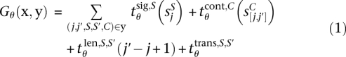Please note that the scores S_j^S and implicitly depend on x via the layer 1 signal predictions. The relative importance of the individual features (i.e., of scores, lengths, and transitions) is adjusted by the transformations t_θ, each of which maps a given feature value to a corresponding score contribution. We will learn these transformations by optimizing their parameterization θ. For the transitions, we have a special case: since t_θ^trans,S,S′ for given states S, S′ does not depend on any additional parameter, the transitions can be represented by a state-by-state transition table t^trans. We model the three other transformations by piecewise linear functions (PLiFs) (Rätsch and Sonnenburg 2007; Rätsch et al. 2007), because they enable efficient training and at the same time are sufficiently expressive to take the relationships between the different features into account. For each PLiF, the supporting points are preselected on the training set according to the range and frequency of occurring feature values. The corresponding function values are learned during global training. Together with the transition table, they define the parameter vector θ. For further details, see Supplemental Section E.5.

Training

For a set of labeled training examples {(xⁿ, yⁿ)}, n = 1,…, N, the parameters θ are tuned such that each true labeling yⁿ scores higher than all other possible labeling by a large margin, i.e., G_θ(xⁿ, yⁿ) >> G_θ(xⁿ, y). To find the optimal parameters θ, the following optimization problem has to be solved (Tsochantaridis et al. 2004):

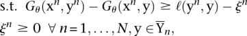where P is a suitable regularizer, the ξ's are slack variables to implement a soft margin (Cortes and Vapnik 1995; Schölkopf and Smola 2002), and ℓ(·,·) is a loss function measuring the difference between label and prediction (details about regularizer and loss are provided in Supplemental Sections E.6.1 and E.6.2).

While the number of constraints in (2) can be enormous, only a small fraction of them is active. Hence, working set methods can be applied in order to solve the problem (Tsochantaridis et al. 2005). The idea is to start with small sets of negative (i.e., false) labelings Y_n^k for every example n in iteration k. One obtains an intermediate solution θ^k for the smaller problem and then identifies labeling that maximally violate the constraints, i.e., 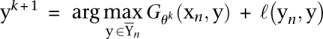. The new constraint generated by the negative labeling is then added to the optimization problem 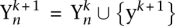. The method described above is also known as the column generation method or cutting-plane algorithm and can be shown to converge to the optimal solution (Hettich and Kortanek 1993; Rätsch 2001; Tsochantaridis et al. 2005).

mGene.multi and mGene.seq: Incorporating additional features

We extended the method described above by including two additional sources of information: genome conservation from multiple genome alignments and prior knowledge in the form of EST or protein alignments. The resulting methods produced predictions submitted to nGASP category 2 and category 3, respectively.

With mGene.multi (dev) we implemented a first version that exploits multiple genome alignments as additional features. For each genomic position j, the corresponding column of the alignment was summarized as a discrete conservation score. This information was subsequently used in two different ways. First, we improved the signal detectors by combining the DNA sequence kernels with additional kernels that act on the corresponding conservation scores in the same windows. Appropriate kernels (linear and/or WD kernels) were chosen during model selection for the individual signals. Second, we designed additional conservation detectors with spectrum kernels that act on the conservation scores within a given segment. The types of conservation detectors are analogous to the content detectors, including one for intergenic, intercistronic, UTR, coding exonic, intronic regions, as well as for the three different reading frames (see Supplemental Sections E.I and E.2 for further details). Together, the improved signal features and the additional conservation features yielded a small performance improvement relative to mGene.init.

For mGene.seq we used EST, cDNA, and protein sequences to support our gene predictions. First, we aligned the sequences against the genome (cf. Supplemental Section E.3). Then, we modified the signal predictions prior to gene structure prediction, i.e., we boosted or suppressed signal predictions that agreed or conflicted, respectively, with the alignments (more details are given in the Supplemental Section E.3). Therefore, in contrast to mGene.multi (dev), one does not need to retrain mGene; only the prediction step has to be repeated.

Additional details on the experimental protocol used for the nGASP competition, as well as the procedure for genome-wide predictions on five nematodes can be found in the Supplemental Sections E.7 and E.9

Availability and resources

We provide two versions of mGene: To enable others to reproduce our results, the source code of the versions of mGene that have been used in this work are available on our website. These versions will be provided under an academic license and support will be limited to reproducing the published results. Additionally, we provide the source code of a mature version of mGene licensed under GPL version 3. It uses a more general model (without trans-splicing and operon predictions) and allows training and prediction on eukaryotic genomes with command line tools. It will be fully supported (see Supplemental Section D). The same version is also available in the mGene.web webservice (Schweikert et al. 2009). Using this system, one may obtain a trained gene-finding model within 24 h: For instance, training signal and content sensors on the nGASP regions, as well as generating layer 1 predictions, takes 2–5 h per individual sensor and can be performed in parallel; the training of the integration step (layer 2) takes about 6 h (see Schweikert et al. 2009 for more details). Using this webserver, we have trained gene predictors for several other genomes including D. melanogaster and A. thaliana (a complete list is available at http://mgene.org/web/performance).

Prediction verification by RT-PCR and sequencing

To verify mGene's predictions, we sampled from predicted spliced genes that did not overlap with any gene from the WS180 annotation. Additionally, we examined a group of spliced annotated, but unconfirmed genes that did not overlap with any mGene prediction (see Supplemental Section F for further details on the target selection). For the selected genes, we designed primer pairs in the first and last coding exon, such that each product spanned at least one intron. Wild-type C. elegans mRNA was reverse transcribed, followed by touchdown PCR. Amplification products were analyzed by gel electrophoresis. All visible gel bands were eluted and sequenced from both sides. The resulting sequences were aligned to the genome using BLAT (Kent 2002) and the experiment was counted as a success if the sequence could be unambiguously mapped to the targeted gene (see Supplemental Section F for further details).

Domain content annotation of new genes

We annotated the protein sequences of the novel C. elegans gene predictions, which are not part of the current WormBase annotations, with InterPro domain predictions. All domain predictions are based on the InterPro collection of protein domain databases (release 16.2) (Hunter et al. 2008). Protein domain predictions were computed with the iprscan application (version 4.3.1) using default parameters (Zdobnov and Apweiler 2001).

Comparative analysis of the gene complement in five nematodes

We initially computed all pairwise BLAST matches with a score cutoff of ≥50 bits (BLO-SUM62 matrix). These pairwise similarity relations served as input to Inparanoid (Remm et al. 2001), which computed all pairwise orthologous clusters for every species pair. We used the proteome of Escherichia coli as an outgroup in our Inparanoid analysis (all sequenced Caenorhabditis species were raised on E. coli cultures), thereby avoiding spurious grouping of potential sequence contaminants. We activated the bootstrapping function of Inparanoid to reject clusters of orthologs with weak support. Subsequently, we used Multiparanoid (Alexeyenko et al. 2006) to generate groups of orthologous genes for multiple species. All programs were run with default parameters if not stated otherwise.

References

- Alexeyenko A, Tamas I, Liu G, Sonnhammer EL. Automatic clustering of orthologs and inparalogs shared by multiple proteomes. Bioinformatics. 2006;22:e9–e15. doi: 10.1093/bioinformatics/btl213. [DOI] [PubMed] [Google Scholar]
- Allen JE, Majoros WH, Pertea M, Salzberg SL. JIGSAW, GeneZilla, and GlimmerHMM: Puzzling out the features of human genes in the encode regions. Genome Biol. 2006;7:S9. doi: 10.1186/gb-2006-7-sl–s9. [DOI] [PMC free article] [PubMed] [Google Scholar]
- Altun Y, Tsochantaridis I, Hofmann T. Hidden Markov support vector machines. Scientific Commons; St. Gallen, Switzerland: 2003. [Google Scholar]
- Ben-Hur A, Ong CS, Sonnenburg S, Scholköpf B, Rätsch G. Support vector machines and kernels for computational biology. PLoS Comput Biol. 2008;4:e1000173. doi: 10.1371/journal.pcbi.1000173. [DOI] [PMC free article] [PubMed] [Google Scholar]
- Bernal A, Crammer K, Hatzigeorgiou A, Pereira F. Global discriminative learning for higher-accuracy computational gene prediction. PLoS Comput Biol, 2007;3:e54. doi: 10.1371/journal.pcbi.0030054. [DOI] [PMC free article] [PubMed] [Google Scholar]
- Brent MR. Steady progress and recent breakthroughs in the accuracy of automated genome annotation. Nat Rev Genet. 2008;9:62–73. doi: 10.1038/nrg2220. [DOI] [PubMed] [Google Scholar]
- Brown RH, Gross SS, Brent MR. Begin at the beginning: Predicting genes with 5′ UTRs. Genome Res. 2005;15:742–747. doi: 10.1101/gr.3696205. [DOI] [PMC free article] [PubMed] [Google Scholar]
- Burge CB, Karlin S. Finding the genes in genomic DNA. Curr Opin Struct Biol. 1998;8:346–354. doi: 10.1016/s0959-440x(98)80069-9. [DOI] [PubMed] [Google Scholar]
- The C. elegans Sequencing Consortium. Genome sequence of the nematode C. elegans: A platform for investigating biology. Science. 1998;282:2012–2018. doi: 10.1126/science.282.5396.2012. [DOI] [PubMed] [Google Scholar]
- Coghlan A, Fiedler TJ, McKay SJ, Flicek P, Harris TW, Blasiar D. nGASP—the nematode genome annotation assessment project. BMC Bioinformatics. 2008;9:549. doi: 10.1186/1471-2105-9-549. [DOI] [PMC free article] [PubMed] [Google Scholar]
- Cortes C, Vapnik VN. Support vector networks. Mach Learn. 1995;20:273–297. [Google Scholar]
- DeCaprio D, Vinson JP, Pearson MD, Montgomery P, Doherty M, Galagan JE. Conrad: Gene prediction using conditional random fields. Genome Res. 2007;17:1389–1398. doi: 10.1101/gr.6558107. [DOI] [PMC free article] [PubMed] [Google Scholar]
- Dieterich C, Clifton SW, Schuster LN, Chinwalla A, Delehaunty K, Dinkelacker I, Fulton L, Fulton R, Godfrey J, Minx P, et al. The Pristionchus pacificus genome provides a unique perspective on nematode lifestyle and parasitism. Nat Genet. 2008;40:1193–1198. doi: 10.1038/ng.227. [DOI] [PMC free article] [PubMed] [Google Scholar]
- Foissac S, Schiex T. Integrating alternative splicing detection into gene prediction. BMC Bioinformatics. 2005;6:25. doi: 10. 1186/1471-2105-6-25. [DOI] [PMC free article] [PubMed] [Google Scholar]
- Gerischer U, editor. Acinetobacter molecular biology. Caister Academic Press; Norwich, UK: 2008. [Google Scholar]
- Gerstein MB, Bruce C, Rozowsky JS, Zheng D, Du J, Korbel JO, Emanuelsson O, Zhang ZD, Weissman S, Snyder M. What is a gene, post-ENCODE? History and updated definition. Genome Res. 2007;17:669–681. doi: 10.1101/gr.6339607. [DOI] [PubMed] [Google Scholar]
- Graber JH, Salisbury J, Hutchins LN, Blumenthal T. C. elegans sequences that control trans-splicing and operon pre-mRNA processing. RNA. 2007;13:1409–1426. doi: 10.1261/rna.596707. [DOI] [PMC free article] [PubMed] [Google Scholar]
- Gross SS, Brent MR. Using multiple alignments to improve gene prediction. J Comput Biol. 2006;13:379–393. doi: 10.1089/cmb.2006.13.379. [DOI] [PubMed] [Google Scholar]
- Gross SS, Do CB, Sirota M, Batzoglou S. CONTRAST: A discriminative, phylogeny-free approach to multiple informant de novo gene prediction. Genome Biol. 2007;8:R269. doi: 10.1186/gb-2007-8-12-r269. [DOI] [PMC free article] [PubMed] [Google Scholar]
- Guigó R, Flicek JF, Abril P, Reymond A, Lagarde J, Denoeud F, Antonarakis S, Ashburner M, Bajic VB, Birney E, et al. EGASP: The human ENCODE genome annotation assessment project. Genome Biol. 2006;7:s1. doi: 10.1186/gb-2006-7-s1-s2. [DOI] [PMC free article] [PubMed] [Google Scholar]
- Hettich R, Kortanek KO. Semi-infinite programming: Theory, methods and applications. SIAM Rev. 1993;3:380–429. [Google Scholar]
- Hunter S, Apweiler R, Attwood TK, Bairoch A, Bateman A, Binns D, Bork P, Das U, Daugherty L, Duquenne L, et al. InterPro: The integrative protein signature database. Nucleic Acids Res. 2008;37:D211–D215. doi: 10.1093/nar/gkn785. [DOI] [PMC free article] [PubMed] [Google Scholar]
- Keerthi SS, Sundararajan S. Technical report, Yahoo Research; 2007. CRF versus SVM-struct for sequence labeling. http://www.keerthis.com/crf_comparison_keerthi_07.pdf. [Google Scholar]
- Kent WJ. BLAT—the BLAST-like alignment tool. Genome Res. 2002;12:656–664. doi: 10.1101/gr.229202. [DOI] [PMC free article] [PubMed] [Google Scholar]
- Kiontke K, Sudhaus W. Ecology of Caenorhabditis species. WormBook. 2006;9:1–14. doi: 10.1895/wormbook.l.37.1. [DOI] [PMC free article] [PubMed] [Google Scholar]
- Korf I. Gene finding in novel genomes. BMC Bioinformatics. 2004;5:59. doi: 10.1186/1471-2105-5-59. [DOI] [PMC free article] [PubMed] [Google Scholar]
- Kulp D, Haussler D, Reese MG, Eeckman FH. A generalized hidden Markov model for the recognition of human genes in DNA. Proc Int Conf Intell Syst Mol Biol. 1996;4:134–142. [PubMed] [Google Scholar]
- Leslie C, Eskin E, Noble WS. The spectrum kernel: A string kernel for SVM protein classification. In: Altman RB, et al., editors. World Scientific. Pacific Symposium on Biocomputing; River Edge, NJ: 2002. pp. 564–575. [PubMed] [Google Scholar]
- Liu H, Han H, Li J, Wong L. An in silico method for prediction of polyadenylation signals in human sequences. Genome Inform. 2003;14:84–93. [PubMed] [Google Scholar]
- Ng AY, Jordan MI. On discriminative vs. generative classifiers: A comparison of logistic regression and naïve Bayes. In: Dietterich TG, et al., editors. Advances in neural information processing systems 14. Vols. 1 and 2. MIT Press; Cambridge, MA: 2002. pp. 841–848. [Google Scholar]
- Rätsch G. University of Potsdam; Germany: 2001. “Robust boosting via convex optimization.”. PhD thesis, [Google Scholar]
- Rätsch G, Sonnenburg S. Large-scale hidden semi-Markov SVMs. In: Schölkopf B, et al., editors. Advances in neural information processing systems. Vol. 19. MIT Press; Cambridge, MA: 2007. pp. 1161–1168. [Google Scholar]
- Rätsch G, Sonnenburg S, Schölkopf B. RASE: Recognition of alternatively spliced exons in C. elegans. Bioinformatics. 2005;21(Suppl. 1):i369–i377. doi: 10.1093/bioinformatics/bti1053. [DOI] [PubMed] [Google Scholar]
- Rätsch G, Sonnenburg S, Schäfer C. Learning interpretable SVMs for biological sequence classification. BMC Bioinformatics. 2006;7(Suppl. 1):S9. doi: 10.1186/1471-2105-7-S1-S9. [DOI] [PMC free article] [PubMed] [Google Scholar]
- Rätsch G, Sonnenburg S, Srinivasan J, Witte H, Müller K-R, Sommer R, Schökopf B. Improving the Caenorhabditis elegans genome annotation using machine learning. PLoS Comput Biol. 2007;3:e20. doi: 10.1371/journal.pcbi.0030020. [DOI] [PMC free article] [PubMed] [Google Scholar]
- Reese MG, Hartzell G, Harris NL, Ohler U, Abril JF, Lewis SE. Genome annotation assessment in Drosophila melanogaster. Genome Res. 2000;10:483–501. doi: 10.1101/gr.10.4.483. [DOI] [PMC free article] [PubMed] [Google Scholar]
- Remm M, Storm CE, Sonnhammer EL. Automatic clustering of orthologs and in-paralogs from pairwise species comparisons. J Mol Biol. 2001;314:1041–1052. doi: 10.1006/jmbi.2000.5197. [DOI] [PubMed] [Google Scholar]
- Salamov AA, Solovyev VV. Ab initio gene finding in Drosophila genomic DNA. Genome Res. 2000;10:516–522. doi: 10.1101/gr.10.4.516. [DOI] [PMC free article] [PubMed] [Google Scholar]
- Sarawagi S, Cohen WW. Semi-Markov conditional random fields for information extraction. In: Saul LK, et al., editors. Advances in neural information processing systems; Proceedings of the 2004 conference. Vol. 17. MIT Press; Cambridge, MA: 2004. [Google Scholar]
- Schölkopf B, Smola AJ. Learning with kernels. MIT Press; Cambridge, MA: 2002. [Google Scholar]
- Schweikert G, Behr J, Zien A, Zeller G, Ong CS, Sonnenburg S, Raetsch G. mGene.web: A web service for accurate computational gene finding. Nucleic Acids Res. 2009;37:W312–W316. doi: 10.1093/nar/gkp479. [DOI] [PMC free article] [PubMed] [Google Scholar]
- Siepel A, Diekhans M, Brejova B, Langton L, Stevens M, Comstock CLG, Davis C, Ewing B, Oommen S, Lau C, et al. Targeted discovery of novel human exons by comparative genomics. Genome Res. 2007;17:1763–1773. doi: 10.1101/gr.7128207. [DOI] [PMC free article] [PubMed] [Google Scholar]
- Sonnenburg S, Zien A, Rätsch G. ARTS: Accurate recognition of transcription starts in human. Bioinformatics. 2006;22:e472–e480. doi: 10.1093/bioinformatics/btl250. [DOI] [PubMed] [Google Scholar]
- Sonnenburg S, Rätsch G, Rieck K. Large-scale learning with string kernels. In: Bottou L, et al., editors. Large-scale kernel machines. MIT Press; Cambridge, MA: 2007a. pp. 73–104. Chapter 4. [Google Scholar]
- Sonnenburg S, Schweikert G, Philips P, Behr J, Rätsch G. Accurate splice site prediction using support vector machines. BMC Bioinformatics. 2007b;8 doi: 10.1186/1471-2105-8-S10-S7. [DOI] [PMC free article] [PubMed] [Google Scholar]
- Stanke M, Schoffmann O, Morgenstern B, Waack S. Gene prediction in eukaryotes with a generalized hidden Markov model that uses hints from external sources. BMC Bioinformatics. 2006;7:62. doi: 10.1186/1471-2105-7-62. [DOI] [PMC free article] [PubMed] [Google Scholar]
- Stein LD, Bao Z, Blasiar D, Blumenthal T, Brent MR, Chen N, Chinwalla A, Clarke L, Clee C, Coghlan A, et al. The genome sequence of Caenorhabditis briggsae: A platform for comparative genomics. PLoS Biol. 2003;1:E45. doi: 10.1371/journal.pbio.0000045. [DOI] [PMC free article] [PubMed] [Google Scholar]
- Sternberg PW, Waterston RH, Speith J, Eddy SR, Wilson RK. National Human Genome Research Institute; 2003. Genome sequence of additional Caenorhabditis species: Enhancing the utility of C. elegans as a model organism. http://www.genome.gov/Pages/Research/Sequencing/SeqProposals/CaenorhabditisSEQ.pdf. [Google Scholar]
- Stormo GD, Haussler D. Optimally parsing a sequence into different classes based on multiple types of evidence. Proc Int Conf Intell Mol Biol. 1994;2:369–375. [PubMed] [Google Scholar]
- Tsochantaridis I, Hofmann T, Joachims T, Altun Y. Support vector machine learning for interdependent and structured output spaces. ACM international conference proceedings series; Proceedings of the twenty-first international conference on machine learning; ACM, Alberta, Canada. 2004. [Google Scholar]
- Tsochantaridis I, Hofmann T, Joachims T, Altun Y. Large-margin methods for structured output spaces. J Mach Learn Res. 2005;6:1453–1484. [Google Scholar]
- Wu CH, Apweiler R, Bairoch A, Natale DA, Barker WC, Boeckmann B, Ferro S, Gasteiger E, Huang H, Lopez R, et al. The universal protein resource (uniprot): An expanding universe of protein information. Nucleic Acids Res. 2006;34:D187–D191. doi: 10.1093/nar/gkj161. [DOI] [PMC free article] [PubMed] [Google Scholar]
- Zdobnov EM, Apweiler R. InterProScan—an integration platform for the signature-recognition methods in InterPro. Bioinformatics. 2001;17:847–848. doi: 10.1093/bioinformatics/17.9.847. [DOI] [PubMed] [Google Scholar]
- Zien A, Rätsch G, Mika S, Schölkopf B, Lengauer T, Müller K-R. Engineering support vector machine kernels that recognize translation initiation sites. Bioinformatics. 2000;16:799–807. doi: 10.1093/bioinformatics/16.9.799. [DOI] [PubMed] [Google Scholar]