Structure of deviations from optimality in biological systems

Abstract

Optimization theory has been used to analyze evolutionary adaptation. This theory has explained many features of biological systems, from the genetic code to animal behavior. However, these systems show important deviations from optimality. Typically, these deviations are large in some particular components of the system, whereas others seem to be almost optimal. Deviations from optimality may be due to many factors in evolution, including stochastic effects and finite time, that may not allow the system to reach the ideal optimum. However, we still expect the system to have a higher probability of reaching a state with a higher value of the proposed indirect measure of fitness. In systems of many components, this implies that the largest deviations are expected in those components with less impact on the indirect measure of fitness. Here, we show that this simple probabilistic rule explains deviations from optimality in two very different biological systems. In Caenorhabditis elegans, this rule successfully explains the experimental deviations of the position of neurons from the configuration of minimal wiring cost. In Escherichia coli, the probabilistic rule correctly obtains the structure of the experimental deviations of metabolic fluxes from the configuration that maximizes biomass production. This approach is proposed to explain or predict more data than optimization theory while using no extra parameters. Thus, it can also be used to find and refine hypotheses about which constraints have shaped biological structures in evolution.

Optimization theory has been widely used to analyze evolutionary adaptation (1–29). Despite their success at explaining important features of many biological systems, optimization principles have been criticized for being an excessive simplification of evolution (30, 31). Major factors in evolution not taken into account by optimization theory are, for example, stochasticity, genetic drift, insufficient time to reach the optimum, the existence of local maxima or insufficient genetic variability (3, 25–31). Practitioners of optimization theory answer to this objection that it is not claimed that biological systems are optimal, but that the optimal configuration is a useful reference to study adaptation in biological systems (3). However, in practical applications the following problem arises: When the real system deviates from the optimum, instead of acknowledging that the system is suboptimal, typically a new optimization principle using more parameters can be given to better fit the data. Although this approach might be justified on the grounds that our objective functions need improvement, the problem is that there is no procedure to distinguish deviations that can be explained by nonadaptive factors like stochasticity or finite time in evolution from those that must be explained by improvement of the objective function.

Here, we test a simple rule for the structure of suboptimal biological systems. This rule implies that the components of the system with lesser impact on the objective function are expected to have a higher probability of deviating from the optimum. We test this theoretical result in the neuroanatomy of the nematode Caenorhabditis elegans. We correctly obtain the structure of deviations from the minimum wiring configuration. We develop a significance test to check that experimental deviations from optimality correspond to the theoretical pattern. Also, a Bayesian approach is given to estimate better objective functions using the data, taking into account the deviations from optimality. Finally, we test the theoretical result in the metabolic network of Escherichia coli. We find that although maximization of ATP and biomass production gives similar predictions in deterministic optimization, it is biomass production that best explains the deviations from the optimum.

Results

Suboptimal Structure in Biological Systems.

Deterministic optimization theory finds the system state x→ with the highest value of the objective function Z(x→). Many factors in evolution, including stochastic effects and finite time, may not allow the system to reach the ideal optimum. In these cases, and given that we typically do not have enough details about these factors, it is still reasonable to expect that the system has a higher probability of reaching a state of high Z. In mathematical terms, we can then write the probability P(x→) of finding the system state x→ as a function f that increases with the objective Z(x→),

We have applied Eq. 1 to systems of many components, such as neurons in a neuronal circuit or chemical fluxes in a metabolic network. In these systems, we typically have that the objective changes differently in the directions of some components than in the direction of others. This is illustrated in Fig. 1A for the case of a toy system of two components. The objective function falls more slowly in the direction of x₁, and Eq. 1 implies then a higher probability of deviating from the optimum for component 1. Analogously, in systems of many components, we expect larger deviations in the components with smaller impact on the objective.

Fig. 1.

Suboptimal structure in a two-component model with objective Z(x₁,x₂) = x₁² + 5x₂². (A) (Upper) Parabolic objective function with slower decrease in the x₁ direction. (Lower) Probability resulting from Eq. 1, using as an example P(x→) = exp(−Z(x→)/0.4). The region of high probability extends further in the direction of x₁ because the objective decreases slower in this direction. (B) (Upper) Contour plots for the objective function (grayscale, lighter for higher values). (Lower) Contour plot for the probability (grayscale, lighter for higher values). Eq. 1 implies that isoprobability lines are the same than isoobjective lines.

Irrespective of the form of function f, Eq. 1 implies a particular structure of the deviations from optimality. This can be seen in Fig. 1B for the 2D case, where we illustrate that the isoprobability lines must be identical to the isoobjective lines, independently of the function f. We can thus systematically use Eq. 1 to explain or predict structure of deviations from optimality, with no need of determining a specific function f, and therefore using no more parameters than those of the objective function.

Before using Eq. 1 to explain experimental deviations from optimality, we checked that it corresponds to the resulting probability in simple models of optimization for finite time or in presence of stochastic factors. To model stochasticity, representing either our ignorance of the many unknown extra factors affecting fitness or true system fluctuations, we may consider a stochastic version of the objective, that is the sum of the deterministic objective and a random variable independent of the system variables. The probability of finding an optimum is higher in the direction in which the objective is also higher because in this direction the stochastic component has a higher probability of producing a new global maximum, resulting in Eq. 1 (see SI Appendix). For the more complex case with stochasticity present and with the system state changing according to local information of the objective surface, like in stochastic hill climbing (32) (Materials and Methods), the probability at equilibrium is again only a function of the objective function, SI Appendix. The effect of finite time may be modeled in a simple way as random jumps among system states for a short time and selecting among them the state with highest value of the objective. Again, the probability can only depend on the objective function, Eq. 1 (see SI Appendix).

Deviations from Optimality in the Neuroanatomy of C. elegans.

We then tested whether the organization of C. elegans neuroanatomy corresponds to the suboptimal structure given by Eq. 1. C. elegans is a nematode whose nervous system consists of about 300 neurons. The principle of wiring economy states that the neurons will be in the positions that minimize the cost of the wire needed to connect them (refs. 18–21; Materials and Methods). Previous theoretical analysis obtained the positions of cell bodies (somas) corresponding to minimum wiring cost, given the observed connectivity (18, 21). The result of this calculation is reproduced in Fig. 2A, showing the good agreement between the optimal and the actual positions of the neurons. However, the system is not optimal (18–21), with ≈15% of neurons showing important deviations from optimality. Here, we used the same wiring cost function as in optimization studies to explain the suboptimal structure of the nervous system. From Eq. 1, deviations from optimality are expected to be larger for the directions of lower cost W(x→) (or equivalently higher objective function, Z(x→) = −W(x→)).

Fig. 2.

Deviations of soma positions in C. elegans from the optimal positions of minimum wiring configuration. (A) Position of somas obtained by deterministic wiring cost minimization versus experimental values. Perfect match between deterministic optimization theory and experiment would fall on the diagonal. (B) Effective number of wires of each neuron (ω) versus experimental deviations from optimality (|Δx| ≡ |x_experimental−x_opt|). Larger deviations are expected for neurons with lower ω. Blue dashed line follows ω ∝ |Δx|⁻², and red solid line follows ω ∝ 1/|Δx|⁻¹. The three outliers (above the red line) are neurons DA6, AVAL, and AVAR. (C) Histogram of the wiring costs resulting from random redistribution of the deviations of somatic positions from their optima. Arrow indicates the cost of the actual configuration. Only 0.033% of the permutations have a lower cost. (D) Effective number of wires (ω) versus deviations obtained from a simulation performed by stochastic hill climbing with a Gaussian stochastic component added to wiring cost. Blue dashed line corresponds to the approximate theoretical prediction, ω ∝ |Δx|⁻².

The wiring cost in the direction of each neuron position is found to increase faster the more wires that neuron has

with ω_i a measure of the number of wires associated with neuron i (see SI Appendix for a proof of this result). Thus, cost grows parabolically with the distance from the soma to its optimal position x_i^opt. Neurons with a lower value of the number of wires ω_i have a slower increasing parabola and are therefore expected to deviate more. This is clearly seen in the experimental data, Fig. 2B. All neurons with large deviations from the optimum have a low number of wires. The frontier of the experimental pattern is well described by ω ∝ 1/|Δx| for all 279 neurons except the three known as DA6, AVAL, and AVAR (Fig. 2B, solid line).

Next, we calculated how significantly these experimental deviations follow the theoretical pattern in Eq. 1 by using the following procedure. Eq. 1 predicts largest deviations to be in the components of the system with lower impact on the cost (neurons with fewer connections). A random reassignation of deviations among neurons is then expected to destroy this effect, increasing the wiring cost. Thus, we randomly redistributed the experimental deviations among the 279 neurons, and calculated how often the cost of the new configuration was lower than the actual one (Materials and Methods). This proportion of cases can be directly treated as a P value, because it is equal to the probability that random deviations get distributed by chance in a way as consistent with our probabilistic model as the empirical data. We found that the experimental deviations correspond very significantly to the probabilistic result, P = 0.00033, Fig. 2C.

We have also tested that alternative hypotheses cannot explain the experimental data shown in Fig. 2B. We checked that the pattern is not due to sampling effects. We also discarded the possibility that experimental errors in the measurement of the positions of neurons, sensors, or muscles are responsible for the structure of the deviations. Finally, we checked that errors in the connectivity matrix cannot explain the data (SI Appendix).

Further insight into the experimental deviations in Fig. 2B can be obtained from a simulation using the algorithm of stochastic hill climbing with Gaussian noise, Fig. 2D. Again, only neurons with low number of wires show important deviations. An approximate theoretical expression for the shape of this pattern can also be obtained from Eq. 1. Assuming independent neurons, that is, each neuron contributing with a term like Eq. 2 to the total wiring cost, and making the change of variable u = $\sqrt{\omega }$Δx, each neuron has the same impact in the wiring cost expressed in the scaled variables and, by Eq. 1, also in the probability or the cumulative probability. Their isolines then correspond in the old variables to ω ∝ 1/|Δx|² (see SI Appendix for a complete proof and tests). As the envelope of the numerical results corresponds to an isoline of the cumulative probability, it follows this expected relationship (Fig. 2D, dashed line). The wiring cost function used until now assumes for simplicity that the cost increases with the square of wire length (18, 21) (see Materials and Methods). For a wiring cost increasing as wire length to any power ξ, the pattern of deviations approximately obeys ω ∝ 1/|Δx|^ξ, always with largest deviations in neurons with lesser number of wires (SI Appendix). For the experimental data in Fig. 2B, the quadratic case gives a reasonable limit for the pattern (Fig. 2B, dashed line), but it is better described by the linear case (Fig. 2B, solid line).

Analysis of the experimental deviations in Fig. 2B shows that they significantly follow Eq. 1 for a wiring cost previously used in deterministic optimization theory (18, 21). Another use of Fig. 2B could be to find the wiring cost exponent best fitting the experimental pattern. However, this use of Fig. 2B would face important limitations. For example, Fig. 2B picks out ω as a relevant parameter to study deviations, but its relevance is only valid close to wiring cost exponent 2 (SI Appendix). Also, a more quantitative use of Eq. 1 requires taking into account the full distribution of the data and not the simple quantities that can be obtained from Fig. 2B, like the envelope or mean of the pattern of deviations. Fig. 2B thus allows for a robust qualitative picture, but a quantitative fitting approach must use Eq. 1 and the full data. For this reason, we built a Bayesian estimator that finds the parameters of the objective function that best fit the data to the probability in Eq. 1. Whereas all of the other procedures presented in this article have predictive value and only use the shape of the objective function, the Bayesian estimator is a fitting procedure that uses extra parameters to describe function f. In order not to make any assumptions about function f, the Bayesian estimator takes into account a wide range of functions, only limited by computational time. A complete description of the Bayesian estimator can be found in SI Appendix.

We have used the Bayesian estimator for the wiring cost for C. elegans, which has three parameters: α, β and the cost exponent ξ (18, 21) (see Materials and Methods). α and β are parameters that weight differently the connections of sensory neurons, interneurons, and motorneurons. There is already an anatomical reason for these weights. We need to transform the connectivity data expressed as number of synapses between any two neurons into number of wires by taking into account the actual anatomy of C. elegans. Actual neurites that connect two neurons or a neuron and a muscle hold on average 29.3 synapses, whereas neuron-sensor wires only hold one synapse. This anatomical difference may be taken into account by making α = β = 1/29.3 (ref. 18; Materials and Methods). However, so far we have used α = 0.05 and β = 1.5, which are known to best fit the C. elegans data within deterministic optimization theory (21). We have used these values to show that objective functions successful in optimization studies can be used to obtain deviations from optimality. For these values, the Bayesian estimator gives the most probable wiring cost exponent of ξ = 1.3 ± 0.09, consistent with our preliminary analysis in Fig. 2B. Also, the significance of the pattern for exponent 1.3 is P = 4·10⁻⁷, much better than for the case of quadratic cost.

However, the α and β that are best for deterministic optimization do not need to be the best from the probabilistic point of view. Therefore, we used the Bayesian estimator to find simultaneously the α, β, and ξ that best fit the data to Eq. 1. We obtain that the most probable α and β (Fig. 3A) are close to the anatomically based values, α = β = 1/29.3 (18) (Fig. 3A, white dot). The most probable cost exponent is ξ = 0.49 ± 0.07(SD) (Fig. 3B, blue line). Also, fixing α and β to the anatomically based values, the Bayesian estimator finds the same wiring cost exponent ξ = 0.49 ± 0.07 (SD) (Fig. 3B, red dashed line). In fact, a cost exponent of ξ ≈ 0.5 is the most probable for all but the least probable α and β values, SI Appendix. Furthermore, by using these estimated parameters, there is an increase of significance, P ≈ 10⁻²³. Similarly to the cases of linear and quadratic cost exponents, for ξ ≈ 0.5 the most deviated neurons correspond to directions of flatter wiring cost, Fig. 3 C and D. A more specific feature of wiring cost with ξ < 1 is that it has local minima in the direction of some neurons. This explains the position of neurons like AVAL and AVAR that are now close to a local minimum (Fig. 3E) and for which linear and quadratic wiring costs gave no explanation (Fig. 2B). However, the improvement is not only for these special neurons. To show this, we checked that we obtained again the same cost exponent, ξ = 0.49 ± 0.06, using in the Bayesian method all neurons except the three outliers in Fig. 2B, DA6, AVAL, and AVAR.

Fig. 3.

Bayesian estimation of parameters in wiring cost function of C. elegans. (A) Probability of α (relative weight for neuron–neuron connections) and β (relative weight for neuron–muscle connections), according to the Bayesian estimator. Most probable values are α = 0.08, β = 0.13. These values are closer to the ones based on C. elegans anatomy, α = β = 1/29.3 (white dot), than to the ones fitting best the data by using deterministic wiring minimization, α = 0.05, β = 1.5 (red plus sign). (B) Probability for the cost exponent ξ. Most probable cost exponent is ξ = 0.49 ± 0.07. Results are identical using the complete Bayesian estimation taking into account all values of α, β (blue) as when fixing α, β to their anatomically based values, α = β = 1/29.3 (red). (C–E) Wiring cost along the direction of the position of neurons ALML, AIZL, and AVAL with all other neurons fixed in their experimental positions, for wiring cost exponents ξ = 0.5 (red), ξ = 1.0 (green), and ξ = 2.0 (blue). Black vertical bars: actual soma position. AVAL is far from its optimal position but sits close to a local minimum. The same happens for AVAR (data not shown). DA6 does not improve significantly with the new parameters.

Deviations from Optimality in the Metabolism of E. coli.

As a second system to test whether Eq. 1 can obtain the suboptimal structure of biological systems, we chose the metabolism of bacterium E. coli. It consists of a network of chemical reactions that transform substances in the medium (glucose, oxygen, etc.) into those needed for the bacterium (ATP, amino acids, etc.). Reconstructions of this network are available from biochemical and genetic studies (8–13) (Materials and Methods). Thus, we know which reactions take part in the bacterium's metabolism and their stoichiometry. The metabolism is also characterized by the reaction fluxes (or rates). For a given reaction, its flux is the number of molecules of reactants, weighted by their stoichiometric coefficients, that are transformed into products each hour, per gram of bacterial culture (dry weight). These fluxes are controlled by the amount of enzymes of each type produced by the bacterium and have been proposed to be tuned to maximize production of biomass for bacterial growth while producing just enough ATP for maintenance of bacterial functions (8–13). The set of fluxes that are consistent with the stoichiometry of the reactions and maximize biomass production can be computed by linear programming (Materials and Methods). The fluxes predicted in this way are in general consistent with experimental results, Fig. 4A. It has been proposed that a better predictor of reaction fluxes may be the maximization of ATP production while maintaining a certain growth rate (13). Under the circumstances considered here, maximization of ATP gives a prediction (Fig. 4B) very similar to that of maximization of biomass (Fig. 4A). This is reasonable, because ATP is one of the most important components of biomass (see Materials and Methods), so maximizing biomass implies having a high ATP production. However, although both objectives seem to have their maximum at very similar configurations, we expected the two surfaces to be different enough to predict different deviations from optimality.

Fig. 4.

Deviations from optimality in the metabolic network of E. coli. (A) Optimal fluxes for maximization of biomass production versus experimental fluxes. Perfect correspondence of deterministic optimization and data would fall in the diagonal. Bars give experimental error reported in ref. 37. (B) Optimal fluxes for maximization of ATP production versus experimental fluxes. (C) Theoretical and experimental deviations from the optimum for biomass production as objective. For each flux, colors show the value of the objective function (relative to the optimum) as a function of the deviation of the flux. Dark red is reserved for a value of objective of exactly 1, so that maxima are clearly seen. Eq. 1 implies that the fluxes should be at the red regions. White dots are located at the experimental deviations. (D) Same as C for ATP production as objective. (E) P value from significance analysis for all possible values of Δ. Red line: significance of the theoretical results using biomass production as objective. Blue line: using ATP production as objective. Black dashed line: P = 0.05 significance line.

Our analysis has two steps. In the first step, we would like to calculate the value of the objective function in the direction of each flux with the rest fixed. But this is not possible because, in general, varying one flux produces a state that is not compatible with the stoichiometry. To avoid this, we allow the other fluxes to change, but to prevent them from taking unrealistic values, we limit them to an interval Δ around the optimum. Then, we fix the flux under study to one of its feasible values and reoptimize the rest of the system within the intervals allowed by Δ. We repeat this procedure for the whole feasible interval to find the upper bound of the objective in the direction of the flux (see Materials and Methods). This upper bound is represented for each experimental flux in color scale in Fig. 4C. The second step tests whether, as expected from Eq. 1, experimental data (Fig. 4C, white dots) avoids regions where the objective function drops substantially (blue regions in Fig. 4C). Fluxes for which the objective stays high only in a small neighborhood of the optimum are expected to have small deviations. Also, fluxes for which the objective drops faster in one direction than in the other are expected to deviate in the direction of slower drop (e.g., flux gltA is expected to have a small negative deviation, Fig. 4C). These theoretical results, when using biomass as the objective, have a good correspondence with experimental values (Fig. 4C). A significance test was performed by randomly exchanging the deviations among fluxes and calculating the proportion of these configurations with equal or higher average values of the objective, and found P = 0.0058 (see SI Appendix).

We then tested whether the experimental deviations from the configuration of maximal ATP production can be explained by Eq. 1. In this case, experimental deviations were found not to be consistent with the theory (Fig. 4D, see, e.g., flux mdh, which is predicted to be near the optimum but is, in reality, very far away). The significance test fails in this case, P = 0.17. The results presented in Fig. 4 C and D were obtained for Δ = 1.99 mmol/g dry wt per h, which is the minimum value for which calculations can be performed both for biomass and ATP as objective functions. However, it turns out that our main conclusions do not depend on the value of Δ. For any value of Δ, our theoretical results correspond to experimental data when biomass is the objective function (P < 0.04), and not when ATP is the objective function (P > 0.09), Fig. 4E. All of the results presented here correspond to experiments where bacteria have a growth rate 0.1 h⁻¹ (meaning that the bacterial population increases 10% every hour). We further tested that we can obtain the structure of experimental deviations for growth rates of 0.2, 0.3, and 0.4 h⁻¹ (SI Appendix). Results for ATP maximization improve slightly for higher growth rates, but biomass typically also improves and it is always the objective most consistent with the experimental data for any value of Δ.

Discussion

We have tested an approach that explains or predicts the statistical structure of deviations from optimality. Using this approach, we have shown that wiring economy and biomass production can explain the experimental data better than previously expected using deterministic optimization theory. Also, the good agreement with the experimental data suggests that the main structure of deviations from optimality need no extra constraints in the objective function. However, we cannot discard the possibility that further refinement of the objective functions may explain finer details of the experimental data. We also gave a method to calculate how significantly the data follow the theoretical prediction, resulting in a P value. This method does not rely on the extraction of some relevant parameter (ω in the case of C. elegans) and it is thus generally applicable.

The correspondence between deviations from the optimum and the objective function allowed for a better choice of objective function. In the case of C. elegans, whereas wiring cost exponents of values 1 and 2 could correctly obtain the structure of deviations from the optimum, sublinear cost is significantly better. In contrast, previous neuroanatomical studies assumed a wiring cost exponent of a value ≥1 (14–21). At present we do not know which physical processes are contributing most to the wiring cost (i.e., building, maintenance, attenuation, or intracellular transport) to be able to build a realistic model of the origin of a sublinear wiring cost. However, we note that the costs of other better known production or transportation systems, like human-made ones, are in most cases sublinear (an effect that is termed economy of scale for production systems and economy of distance for transportation systems) (38–42).

We believe that the procedures described in this article will be widely applicable to any system for which an optimization principle has been proposed. They allow one to find traces of optimization even in systems far from the optimum and to better select among objective functions. Also, it is possible to use them in systems trapped in a local maximum by studying the shape of the objective function in the neighborhood of that point.

Materials and Methods

Wiring Cost in C. elegans.

An almost complete reconstruction of the nervous system of C. elegans has been obtained from electron microscopy photographs (18, 34, 35). Thus, we know the network connectivity, the soma position for the n = 279 neurons and the S = M = 48 positions of contact between neurites and muscles or sensors. We used a 1D model where each neuron, sensor, or muscle is represented by a point located in the projection of its 3D position on the anteroposterior axis (18). Data are available at www.wormatlas.org. The total wiring cost for C. elegans is (18, 21)

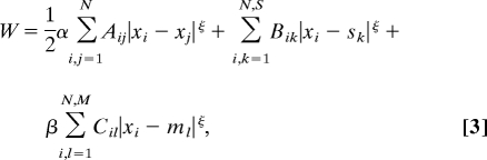where x_i, s_k, and m_l are the positions of neurons, sensors, and muscles, respectively, and A, B, and C are neuron–neuron, neuron–sensor, and neuron–muscle connectivity matrices, respectively. α and β are parameters to take into account differences in average cost of the three kinds of connections. In the actual network, neurites that connect two neurons or a neuron and a muscle hold, on average, 29.3 synapses, whereas neuron–sensor wires only hold one synapse. This anatomical difference may be taken into account by making α = β = 1/29.3 (18). However, optimization theory has shown a better correspondence with experiments for α = 0.05 and β = 1.15 (21). ξ is a nonnegative exponent, previously argued to be ≈2 (17). Therefore, we use ξ = 2, α = 0.05, and β = 1.5, unless otherwise stated.

Deterministic Optimization of C. elegans.

For quadratic cost (ξ = 2), the optimum can be calculated exactly (17, 18, 21). For other exponents, for which no analytical procedure is available, we discretized the worm in 100 bins, computed the cost for each neuron in each position with all other neurons fixed, and selected the bin with lowest cost. Iteration of this algorithm leads to a stationary state in which each neuron is already in the position identified as optimal in the following iteration. In this situation, by construction all partial derivatives will be zero (neglecting the imprecision due to the binning), so the system will be at a local minimum. As the problem is convex for ξ > 1, there is only one local minimum which is also the global minimum. For ξ ≤ 1, we repeat the optimization at least 100 times, starting from random initial conditions, and choose the one ending at lowest cost.

Stochastic optimization of C. elegans was performed by stochastic hill climbing, which consists of adding small random variations to the neurons' positions (we added to each position a random number normally distributed with variance 0.001), and accepting the change only when the new cost plus a random number is lower than the previous cost. We ran 5–10 million iterations, checking that both cost and mean deviation had stabilized, which is necessary to satisfy Eq. 1 in the final configuration (SI Appendix).

Significance Analysis in C. elegans.

The permutation test was performed by using the following algorithm: Build a set of positions by randomly permuting the deviations among the neurons and adding them to the optimal positions. In general, some neurons' positions will be outside the limits of the worm. For each of these neurons, find all other neurons such that interchanging the deviations would result in both neurons inside the worm. Choose randomly one of them, and interchange the deviations. Once all neurons are inside the animal, calculate the cost. We repeated this procedure 10⁷ times for the computation of the P values. Estimation of P values <10⁻⁷ was done by approximating the histogram of permutation's cost by a Gaussian distribution, and calculating its cumulative probability from −∞ to the experimental value.

Stoichiometric Model for the Metabolism of E. coli.

We used a previously published reaction network (13) that, after removal of redundant reactions, is formed by 88 reactions and 60 metabolites. Bacterial growth is incorporated as a reaction consisting in the consumption of metabolites in the proportions measured experimentally in bacterial biomass, and production of the virtual metabolite “Biomass” plus a small amount of subproducts (9) (see Dataset S1 for the meaning of the metabolites' abbreviations),

This is the reaction whose flux is maximized when biomass is the objective function. When ATP is the objective function, we maximize a reaction which just consists of consumption of ATP. The model can be found in Dataset S1, and is described in detail in SI Appendix. We performed linear optimization with the open-source GLPK optimization package (GNU Linear Programming kit; www.gnu.org/software/glpk/), and routines written in Matlab (MathWorks). Our routines are based on COBRA toolbox (36).

Calculation of Maintenance Requirements of E. coli.

Maintenance requirements are modeled as ATP consumption, with two different contributions: Non-growth-associated maintenance (NGAM), and growth associated maintenance (GAM) (9). These two parameters are computed by a fit to the experimental data, making the growth predicted by the model match the experimental growth (9), see SI Appendix. We obtained NGAM = 12.5 mmol of ATP per g dry wt (gDW) per h and GAM = 126 mmol of ATP per gDW. Maintenance is added to the model only when biomass production is the objective function. When ATP is the objective function the network anyway produces as much ATP as possible, and the addition of maintenance requirements makes no difference.

Extra Constraints When ATP Is the Objective Function.

When ATP is the objective function, all of the resources of the metabolic network are diverted to ATP production, resulting in zero growth rate. To avoid this unrealistic situation, when ATP is the objective the growth rate is fixed to its experimental value (13) (see bounds in Dataset S1).

Simulation of Experimental Conditions of E. coli.

Experimental conditions are simulated by fixing some of the secretion/uptake rates (external fluxes). In all cases glucose uptake rate was fixed to the experimental value. We allowed unlimited uptake of other metabolites present in the medium (CO₂, O₂, and NO₃), and unlimited secretion of the rest of external metabolites (see Dataset S1).

Experimental Data of E. Coli Were Taken from Ref. 37.

They correspond to ¹³C labeling experiments on chemostat cultures of E. coli (MG1655 strain). A total of eight experiments are presented, in four groups: three experiments with growth rate ≈0.1 h⁻¹, one experiment with growth rate ≈0.2 h⁻¹, two with growth rate ≈0.3 h⁻¹, and two with growth rate ≈0.4 h⁻¹. For the cases with more than one experiment for the same growth rate, we use the average of the results. These data can be found in Dataset S1.

Calculation of the Upper Bound of the Objective Function in the Direction of Each Flux.

First, we constrain to an interval Δ around their optimum all fluxes, except the one under study, the objective and those fixed previously (such as glucose uptake rate, fixed in its experimental value). Then, we find the maximum value of the objective compatible with these constrains for each value of the flux under study. This value is represented in color scale in Fig. 4 C and D. The feasible interval for the flux under study is larger the higher is Δ. We must select Δ high enough to allow the study of all fluxes with experimental data up to their experimental value. In the case of dilution rate 0.1 h⁻¹, Δ_min = 0.88 mmol/gDW·h when biomass is the objective function, and Δ_min = 1.99 mmol/gDW·h when ATP is the objective function. In the limit Δ → ∞, this calculation is the same as robustness analysis (8, 36). See SI Appendix for further details.

References

- 1.Barton NH, Briggs DEG, Eisen JA, Goldstein DB, Patel NH. Evolution. Cold Spring Harbor, NY: Cold Spring Harbor Lab Press; 2007. [Google Scholar]
- 2.Alexander RM. Optima for Animals. Princeton: Princeton Univ Press; 1996. [Google Scholar]
- 3.Parker GA, Maynard Smith J. Optimality theory in evolutionary biology. Nature. 1990;348:27–33. [Google Scholar]
- 4.Freeland SJ, Hurst LD. The genetic code is one in a million. J Mol Evol. 1998;47:238–248. doi: 10.1007/pl00006381. [DOI] [PubMed] [Google Scholar]
- 5.Itzkovitz S, Alon U. The genetic code is nearly optimal for allowing additional information within protein-coding sequences. Genome Res. 2007;17:405–412. doi: 10.1101/gr.5987307. [DOI] [PMC free article] [PubMed] [Google Scholar]
- 6.Dekel E, Alon U. Optimality and evolutionary tuning of the expression level of a protein. Nature. 2005;430:588–592. doi: 10.1038/nature03842. [DOI] [PubMed] [Google Scholar]
- 7.Tkacik G, Callan CG, Jr, Bialek W. Information flow and optimization in transcriptional regulation. Proc Natl Acad Sci USA. 2008;105:12265–12270. doi: 10.1073/pnas.0806077105. [DOI] [PMC free article] [PubMed] [Google Scholar]
- 8.Palsson BO. Systems Biology: Properties of Reconstructed Networks. Cambridge, UK: Cambridge Univ Press; 2006. [Google Scholar]
- 9.Varma A, Palsson BO. Stoichiometric flux balance models quantitatively predict growth and metabolic by-product secretion in wild-type Escherichia coli W3010. Appl Environ Microbiol. 1994;60:3724–3730. doi: 10.1128/aem.60.10.3724-3731.1994. [DOI] [PMC free article] [PubMed] [Google Scholar]
- 10.Edwards JS, Ibarra RU, Palsson BO. In silico predictions of Escherichia coli metabolic capabilities are consistent with experimental data. Nat Biotechnol. 2001;19:125–130. doi: 10.1038/84379. [DOI] [PubMed] [Google Scholar]
- 11.Ibarra RU, Edwards JS, Palsson BO. Escherichia coli K-12 undergoes adaptive evolution to achieve in silico predicted optimal growth. Nature. 2002;420:186–189. doi: 10.1038/nature01149. [DOI] [PubMed] [Google Scholar]
- 12.Segre D, Vitkup D, Church GM. Analysis of optimality in natural and perturbed metabolic networks. Proc Natl Acad Sci USA. 2002;99:15112–15117. doi: 10.1073/pnas.232349399. [DOI] [PMC free article] [PubMed] [Google Scholar]
- 13.Schuetz R, Kuepfer L, Sauer U. Systematic evaluation of objective functions for predicting intracellular fluxes in Escherichia coli. Mol Syst Biol. 2007;3:119–133. doi: 10.1038/msb4100162. [DOI] [PMC free article] [PubMed] [Google Scholar]
- 14.Chklovskii DB, Schikorski T, Stevens CF. Wiring optimization in cortical circuits. Neuron. 2002;34:341–347. doi: 10.1016/s0896-6273(02)00679-7. [DOI] [PubMed] [Google Scholar]
- 15.Klyachko VA, Stevens CF. Connectivity optimization and the positioning of cortical areas. Proc Natl Acad Sci USA. 2003;100:7937–7941. doi: 10.1073/pnas.0932745100. [DOI] [PMC free article] [PubMed] [Google Scholar]
- 16.Buzsaki G, Geiler C, Henze DA, Wang X-J. Interneuron diversity series: Circuit complexity and axon wiring economy of cortical circuits. Trends Neurosci. 2004;27:186–193. doi: 10.1016/j.tins.2004.02.007. [DOI] [PubMed] [Google Scholar]
- 17.Chklovskii DB. Exact solution for the optimal neuronal layout problem. Neural Comput. 2004;16:2067–2078. doi: 10.1162/0899766041732422. [DOI] [PubMed] [Google Scholar]
- 18.Chen BL, Hall DH, Chklovskii DB. Wiring optimization can relate neuronal structure and function. Proc Natl Acad Sci USA. 2006;103:4723–4728. doi: 10.1073/pnas.0506806103. [DOI] [PMC free article] [PubMed] [Google Scholar]
- 19.Ahn Y-Y, Jeong H, Kim BJ. Wiring cost in the organization of a biological neuronal network. Physica A. 2006;367:430–537. [Google Scholar]
- 20.Kaiser M, Hiltetag CC. Nonoptimal component placement, but short processing paths, due to long-distance projections in neural systems. PloS Comp Biol. 2006;2:e95. doi: 10.1371/journal.pcbi.0020095. [DOI] [PMC free article] [PubMed] [Google Scholar]
- 21.Perez-Escudero A, de Polavieja G. Optimally wired subnetwork determines neuronanatomy of Caenorhabditis elegans. Proc Natl Acad Sci USA. 2007;104:17180–17185. doi: 10.1073/pnas.0703183104. [DOI] [PMC free article] [PubMed] [Google Scholar]
- 22.Laughlin SB. A simple coding procedure enhances a neuron's information capacity. Z Naturforsch. 1981;36c:910–912. [PubMed] [Google Scholar]
- 23.Rieke F, Warland D, Bialek W. Coding efficiency and information rates in sensory neurons. Europhys Lett. 1993;22:151–156. [Google Scholar]
- 24.de Polavieja GG. Errors drive the evolution of biological signalling to costly codes. J Theor Biol. 2002;214:657–664. doi: 10.1006/jtbi.2001.2498. [DOI] [PubMed] [Google Scholar]
- 25.Oaten A. Optimal foraging in patches: a case for stochasticity. Theor Pop Biol. 1977;12:263–285. doi: 10.1016/0040-5809(77)90046-6. [DOI] [PubMed] [Google Scholar]
- 26.Murray CD. The physiological principle of minimum work. I. The vascular system and the cost of blood volume. Proc Natl Acad Sci USA. 1926;12:207–214. doi: 10.1073/pnas.12.3.207. [DOI] [PMC free article] [PubMed] [Google Scholar]
- 27.Murray CD. The physiological principle of minimum work applied to the angle branching of arteries. J Gen Physiol. 1926;9:235–841. doi: 10.1085/jgp.9.6.835. [DOI] [PMC free article] [PubMed] [Google Scholar]
- 28.Weibel ER, Gomez DM. Architecture of the human lung. Science. 1962;137:577–585. doi: 10.1126/science.137.3530.577. [DOI] [PubMed] [Google Scholar]
- 29.Sherman TF. On connecting large vessels to small. J Gen Physiol. 1981;78:431–453. doi: 10.1085/jgp.78.4.431. [DOI] [PMC free article] [PubMed] [Google Scholar]
- 30.Gould SJ, Lewontin RC. The spandrels of San Marco and the panglosian paradigm: A critique of the adaptationist program. Proc R Soc London Ser B. 1979;205:581–598. doi: 10.1098/rspb.1979.0086. [DOI] [PubMed] [Google Scholar]
- 31.Lynch M, Walsh B. Genetics and Analysis of Quantitative Traits. Sunderland, MA: Sinauer; 1998. [Google Scholar]
- 32.Michalewicz Z, Fogel DB. How to Solve It: Modern Heuristics. New York: Springer; 2000. [Google Scholar]
- 33.Kirkpatrick S, Gelatt CD, Vecchi MP. Optimization by simulated annealing. Science. 1983;220:671–680. doi: 10.1126/science.220.4598.671. [DOI] [PubMed] [Google Scholar]
- 34.White JG, Southgate E, Thomson JN, Brenner S. The structure of the nervous system of the nematode Caenorhabditis elegans. Philos Trans R Soc London Ser B. 1986;314:1–340. doi: 10.1098/rstb.1986.0056. [DOI] [PubMed] [Google Scholar]
- 35.Hall DH, Russell RL. The posterior nervous system of the nematode Caenorhabditis elegans: Serial reconstruction of identified neurons and complete pattern of synaptic interactions. J Neurosci. 1991;11:1–22. doi: 10.1523/JNEUROSCI.11-01-00001.1991. [DOI] [PMC free article] [PubMed] [Google Scholar]
- 36.Becker SA, et al. Quantitative prediction of cellular metabolism with constraint-based models: the COBRA toolbox. Nat Protocols. 2007;2:727–738. doi: 10.1038/nprot.2007.99. [DOI] [PubMed] [Google Scholar]
- 37.Nanchen A, Schicker A, Sauer U. Nonlinear dependency of intracellular fluxes on growth rate in miniaturized continuous cultures of Escherichia coli. Appl Environ Microbiol. 2006;72:1164–1172. doi: 10.1128/AEM.72.2.1164-1172.2006. [DOI] [PMC free article] [PubMed] [Google Scholar]
- 38.Haldi J, Whitcomb D. Economies of scale in industrial plants. J Polit Econ. 1967;75:373–385. [Google Scholar]
- 39.Nerlove M. Returns to scale in electricity supply. In: Christ F, et al., editors. Measurement in Economics. Stanford, CA: Stanford Univ Press; 1963. pp. 167–198. [Google Scholar]
- 40.Christensen LR, Greene WH. Economies of scale in U.S. electric power generation. J Polit. 1976;4:655–676. [Google Scholar]
- 41.Janic M. Modelling the full costs of an intermodal and road freight transport network. Transportation Res D. 2007;12:33–44. [Google Scholar]
- 42.McCann P. A proof of the relationship between optimal vehicle size, haulage length and structure of distance-transport costs. Transportation Res A. 2001;35:671–693. [Google Scholar]
Associated Data
This section collects any data citations, data availability statements, or supplementary materials included in this article.