Bi-phase locking — a tool for probing non-linear interaction in the human brain

Abstract

We present a novel method for detecting frequency-frequency coupling between the electrical output of cortical areas as measured by electrocorticography (ECoG), electroencephalography (EEG) and magnetoencephalography (MEG), the biphase-locking value (bPLV). Our method is an extension of the well known phase-locking value (PLV) and is specifically sensitive to non-linear interactions, i.e quadratic phase coupling across frequencies. Due to its sensitivity to non-linear interactions, it is robust to spurious synchronization arising from linear crosstalk, which is an especially useful property when analyzing data recorded by EEG/MEG. We discuss the statistical properties of the bPLV, specifically the distribution of the bPLV under assumption of random phases between the signals of interest. We also compare the bPLV to the PLV for cortical interactions that are computed for simulated EEG/MEG data. These data were mapped to the cortex using an inverse solution. We demonstrate our method for event related ECoG data recorded from the motor cortex of an epileptic patient, who performed a cued finger movement task. We find highly significant, movement related increase of the bPLV between the α (12 Hz) and high γ (77 Hz) band in a pre-motor area, coupling to high γ at 89 Hz in the motor cortex.

Introduction

Large scale synchronization is widely believed to reflect coordination of neuronal assemblies during complex tasks and as such is fundamental in the study of human cognition (Singer, 1993; Kahana, 2006). Therefore, the development of methods for the detection of synchronization in the electrophysiological correlates of neuronal activity, using either invasive methods such as ECoG or noninvasive methods, such as EEG or MEG, is of importance. Presently, the majority of methods has been focused on synchronization within a single frequency or frequency band or on harmonic couplings of those frequencies (Tass et al., 1998; Lachaux et al., 1999; Gross et al., 2001). However, cross-frequency coupling of cortical areas has been the subject of recent studies, using the bicoherence (Nikias and Mendel, 1993), which mixes phase and amplitude relations, between signals (Shils et al., 1996; Schack et al., 2002) or the phase-amplitude relationship between different frequencies (Canolty et al., 2006). It has been shown however that pure phase-phase relationships, i.e. phase synchronizations, between distant cortical sites are important (Rudrauf et al., 2006) and can occur without local amplitude changes (Palva and Palva, 2007). In order to study such phase relationships across frequencies, we introduce a new method to estimate time varying quadratic phase coupling of electrophysiological signals, the bi-phase locking value (bPLV). This measure is sensitive to non-linear interactions, such as multiplication, amplitude modulation or phase modulation, of two signals to another signal. Neuronal generators of such interactions have been shown to exist, e.g. in the cricket, where multiplication of angular speed and size of objects is carried out in single neurons (Gabbiani et al., 2002). Multiplicative interaction is also necessary for the implementation of neuronal control circuits, such as phase-locked-loops, which have been suggested to play a functional role in the sensorimotor system of the rat (Ahissar and Kleinfeld, 2002). Apart from control and purely computational functions, phase or frequency modulation could play a role in cortical information transfer, where a carrier frequency or phase is modulated at one cortical site to transmit information to a distant site.

Here we discuss the bPLV method and its properties in detail. Specifically we present a framework to assess the statistical significance of the measured bPLV. We demonstrate our methods on an exemplary ECoG dataset, using a similar paradigm as in a previous study (Darvas et al., 2009), where we analyzed non-linear interaction during a cued finger movement task in four subjects. We also analyze the performance of our method in a simulation, where we apply it to cortical time series from inverse mappings that were computed from simulated EEG data. Even though we use ECoG and EEG data to demonstrate the method in this paper, it is straightforward to apply our results to MEG as well.

Methods

The bPLV

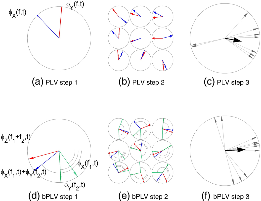
The bPLV is a straightforward generalization of the classical phase-locking value (PLV) that has been introduced by (Lachaux et al. (1999). In analogy to PLV, the bPLV detects synchronization between narrow frequency bands as a function of time. The bPLV is related to the bi-coherence (Nikias and Mendel, 1993) in the same way that PLV is related to coherence (Lachaux et al., 2002), signals are normalized by their analytic amplitudes prior to averaging over trials or time. In both cases, i.e. bPLV and PLV, the resulting measure is time dependent, since it is based on the instantaneous phase of the signal, whereas the typical application of (bi)coherence provides a static measure and requires stationary signals. Also, its independence of the signal amplitude allows the phase locking measures to detect synchronization in situations, where there are no strong and amplitude correlations, thus making them more sensitive than the classical (bi)coherence measures. The bPLV is sensitive to coupling of the phases of two independent frequencies, ϕ₁(f₁,t) and ϕ₂(f₂,t), to the phase of a third frequency, ϕ₃ (f₃,t),f₃ = f₁ + f₂, as shown in Fig. 1, while the PLV is sensitive to the coupling of the phases of the same frequency in two signals.

Fig. 1.

Comparison of the phase locking value (PLV) computation with the biphase locking value (bPLV) computation. The PLV measures the correlation between the phases of two signals at the same frequency f. The bPLV measures the correlation between the phases of three signals at three different frequencies f₁,f₂, and f₃ that are related by f₁ + f₂ = f₃. (a) PLV Step 1. The phase of the signal $X^i(t),{\varphi }_X^i(f,t)$ (shown by blue arrows) and the phase of the signal Yⁱ (t), ϕⁱ_Y (f, t) (shown by red arrows) are extracted from the data for each single trial i at frequency f. (b) PLV Step 2. The phase difference ${\mathrm{\Delta }}_2^i={\varphi }_X^i(f,t)-{\varphi }_Y^i(f,t)$ is then computed for each trial i. (c) PLV Step 3. The PLV is computed as the mean of the single trial phase differences ${\mathrm{\Delta }}_2=\langle {\mathrm{\Delta }}_2^i\rangle$. The single trial phase differences are shown by grey arrows and their mean is shown by the black arrow. (d) bPLV Step 1. The phase of signal $X^i(t),{\varphi }_X^i(f_1,t)$ (shown by blue arrows), the phase of signal $Y^i(t),{\varphi }_Y^i(f_2,t)$ (shown by green arrows), and the phase of signal $Z^i(t),{\varphi }_Z^i(f_3,t)$ (shown by red arrows) are extracted from the data for each single trial i. (e) bPLV Step 2. The phase difference ${\mathrm{\Delta }}_3^i={\varphi }_X^i(f_1,t)+{\varphi }_Y^i(f_2,t)-{\varphi }_Z^i(f_3,t)$ is then computed for each trial i. (f) bPLV Step 3. The bPLV is computed as the mean of the single trial phase differences ${\Delta }_3=\langle {\Delta }_3^i\rangle$. The single trial phase differences are shown by grey arrows and their mean is shown by the black arrow.

This coupling can take place between a pair of frequencies, (f₁,f₂) in one signal, X, to f₃ = f₁ + f₂ in another signal Y or between three separate signals, X, Y and Z. The bPLV can be defined trial-wise over N repetitions of the signals or time-wise over T samples (Hurtado et al., 2004). Typically in an event related EEG/MEG experiment, the N repetitions of each signal correspond to repetitions of the experimental paradigm.

The trial-wise bPLV between three signals is defined as

$$B_{\mathit{\text{XYZ}}}(f_1,f_2,t)=\left|\frac{1}{N}{\displaystyle \sum _{i=1}^N\text{exp}\left(j\right({\varphi }_X^i(f_1,t)+{\varphi }_Y^i(f_2,t)-{\varphi }_Z^i(f_1+f_2,t)\left)\right)}\right|,$$ (1)

where ${\varphi }_X^i(f_1,t)$ is the phase at frequency f₁ in the ith trial.

Similarly, the time-wise bPLV is defined as:

$$\begin{array}{cc}{B}_{\mathit{\text{XYZ}}}(f_1,f_2,t)\hfill & =|\frac{1}{T}{\displaystyle \sum _{\tau =1}^T\text{exp}(j({\varphi }_X(f_1,t-\Delta t\tau )+{/}_Y(f_2,t-\Delta t\tau )}\hfill \\ \hfill & -{\varphi }_Z(f_1+f_2,t-\Delta t\tau )))|,\hfill \end{array}$$

where Δt is the sampling time between two samples. In order to compute the time varying phases of the signals at various frequencies one can either follow the approach outlined in Tass et al. (1998) or Lachaux et al. (1999), i.e. after narrow bandpass filtering the signal X (t) at frequency f, the phase can be computed either by applying the Hilbert transform to the narrow band signal X (f,t) or by convolving it with a Gabor wavelet $G(f,t)=\text{exp}(-\frac{-t^2}{2{\sigma }_t}+j2\pi ft)$, centered at frequency f. Both methods have been shown to perform comparably (Le Van Quyen et al., 2001). Typically, a finite impulse response (FIR) filter is used in order to preserve the phase relation of the bandpass-filtered signals.

A multiplicative non-linearity that produces B_XYZ(f₁,f₂,t) = 1 is given by

• Z(f₁ + f₂,t) = X(f₁,t)Y(f₂,t).

Let X(f,t) = A_X(f,t)exp(jϕ_X(f,t)) be the analytic narrow band signal corresponding to X(f,t), then the above equation yields

• A_Z(f₁ + f₂,t)exp(jϕ_Z (f₁ + f₂,t))

      = A_X(f₁,t)exp(jϕ_X(f₁,t))A_Y(f₂,t)exp(jϕ_Y(f₂,t))

and thus we have

• ϕ_Z(f₁ + f₂,t) = ϕ_X(f₁,t) + ϕ_Y(f₂,t),

which will produce B_XYZ(f₁,f₂,t) = 1 when inserted into Eq. 1. Likewise

• Z(f₁ − f₂,t) = X (f₁,t)Y(−f₂,t),

which leads to

• ϕ_Z(f₁ − f₂,t) = ϕ_X(f₁,t) − ϕ_Y(f₂,t),

yields $B_{\mathit{\text{XYZ}}}^{*}(f_1,f_2,t)=1$, where $B_{\mathit{\text{XYZ}}}^{*}$ is the conjugated bPLV defined as

$$B_{\mathit{\text{XYZ}}}^{*}(f_1,-f_2,t)=\left|\frac{1}{N}{\displaystyle \sum _{i=1}^N\text{exp}\left(j\right({\varphi }_X^i(f_1,t)-{\varphi }_Y^i(f_2,t)-{\varphi }_Z^i(f_1-f_2,t)\left)\right)}\right|.$$

Since a broadband signal can carry independent information in multiple bands, the bPLV does not require three separate signals, X, Y and Z as inputs. The signal X for example can carry information at f₁ and f₂, which couple to f₁ + f₂ in another signal Y and the two-way bPLV for this case is given by B_XXY. Similarly, the cross-frequency coupling can take place solely in one signal, for which we have B_XXX. In analogy to the higher order spectra, i.e. the tri-spectrum and tri-coherence (Nikias and Mendel, 1993), the concept of the bPLV can be extended to nth order phase locking.

Properties of the bPLV

The bPLV has a number of useful properties, which make it well suited to analyze electrophysiological data.

Non-linearity

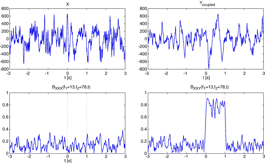
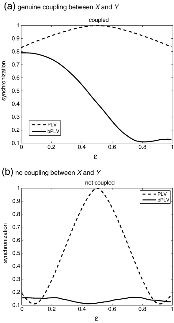
The bPLV measures only non-linear relationships between signals and is thus able to distinguish between linear and genuine non-linear interactions between signals. If we measure the two-way bPLV between two signals X and Y, B_XXY (f₁,f₂,t), where Y = αX, then B_XXY = B_XXX. Unlike symmetric measures of interaction however, B_XXX ≠ 1, because the phases in signal X at frequencies f₁ and f₂ do not necessarily couple to the phase at frequency f₁ + f₂ in X. For phase locking of a signal with itself we have P_XY (f,t) = P_XX (f,t) for Y = αX, where P denotes the PLV and we always have P_XX = 1. This is indistinguishable from the situation of perfect synchronization between X and Y, where we also have P_XY = 1. On the other hand, if there is genuine non-linear coupling between X and Y, it follows that B_XXY ≠ B_XXX and thus the bPLV allows to separate the linear coupling case of Y = αX, where B_XXY = B_XXX from the non-linear coupling case. This relationship is illustrated in Fig. 2, where we show the bPLV between two simulated signals, which are multiplicatively coupled in the interval [0,1]s. We constructed the coupled signal by subtracting from Y the narrow band component Y (f₁ + f₂,t) and then adding the product of narrow band components X (f₁,t)X (f₂,t), normalized by $\sqrt{A_X(f_1,t)A_Y(f_2,t)}$ in the interval [0,1]s, i.e. $Y_{\text{coupled}}=Y-Y(f_1+f_2,t)+X(f_1,t)X(f_2,t)/\sqrt{A_X(f_1,t)A_Y(f_2,t)}$. The original signals were taken from an ECoG recording were the subject performed a cued motor task that was repeated N = 46 times. In this simulation, there is no coupling within X between f₁ and f₂ and hence the bPLV between X and X stays low during the coupling interval, while it is high for the genuine coupling between X and Y. When analyzing electrophysiological data from EEG/MEG or ECoG, linear mixture, or crosstalk, of the true cortical signals in the recording sensors due to volume conduction can lead to false synchronization, as opposed to ‘true’ functional synchronization, that arises solely from brain function. A linear measure, such as PLV, will not be able to distinguish between these types of synchronization. This affects ECoG recordings less, since the ECoG electrodes mostly pick up local potential changes (Miller et al., 2007), but can pose serious problems for EEG/MEG. Fig. 3 illustrates the effects of cross talk in two different situations, (1) where the ‘true’ signals X and Y are genuinely coupled and (2), where there is no coupling between the true signals. The synchronization was computed for the mixed signals X_m = (1−ε)X + εY and Y_m = εX + (1 − ε)Y. Fig. 3(a) shows the different behavior of the bPLV and PLV between X_m and Y_m for increasing ε. Fig. 3(b) shows the effect of crosstalk on sources, which by themselves are not phase or bi-phase coupled. Here, the bPLV, due to its insensitivity to linear interactions, allows to clearly distinguish crosstalk effects from real interactions, because at any degree ε of coupling, the synchronization that the bPLV measures between X_m and Y_m stays low, while the PLV, even at low levels of crosstalk, for example when ε = 0.3, produces synchronization values which are 3 times higher than the true baseline synchronization at ε = 0.

Fig. 2.

bPLV between simulated signals. Top row: The signals X and Y, sampled at 250 Hz over a 6 s period. Bottom row, left: Coupling of X to itself at frequencies (f₁,f₂) = (13,79) Hz to f₃ = 91 Hz. The dotted line shows the interval, where X and Y are bi-phase coupled. Bottom row, right: Coupling of X to Y at the same frequencies.

Fig. 3.

Crosstalk effects on the PLV (dotted line) and the bPLV (solid line) for different degrees of linear mixture. The y-axis shows the synchronization index and the x-axis the linear mixture parameter ε. (a) The PLV and bPLV for the situation where there is genuine coupling between signals X and Y. For the bPLV, two frequencies in X couple to the summed frequency in Y. (b) The PLV and bPLV for the situation, where there is no coupling between X and Y.

Directionality of interaction and causality

The PLV between two signals X and Y, P_XY(f,t) is symmetric with respect to the order of the signals, P_XY(f,t) = P_YX(f,t) whereas the bPLV is generally not. Since we have B_XYZ(f₁,f₂,t) it follows that B_XYZ(f₁,f₂,t) ≠ B_ZXY(f₁,f₂,t) except for the special case where X carries the same phase information as Z at f₁ + f₂ and Z carries the same phase information as X at f₁. This asymmetry allows to use the bPLV as a directional measure, if it is calculated between only two signals, X and Y. In this case, B_XYZ(f₁,f₂,t) reduces to B_XXY(f₁,f₂,t) and its value quantifies the direction of interaction from X to Y, if the phases in X at f₁ and f₂ are independent. In this case X is causal to Y in the Granger (1969) sense, because knowledge of ϕ_X(f₁,t) and ϕ_X(f₂,t) can be used to predict ϕ_Y(f₁ + f₂,t), but not vice versa.

Effect of stimulus locked events

The PLV for stimulus locked data can exhibit an apparent synchronization between cortical sites that does not arise from genuine interaction between these sites. Such apparent or false synchronizations do not even have to be exterior artifacts, e.g. muscle artifacts or eye blinks that are time locked to the stimulus presentation, but can originate from the brain itself. An example would be two independent oscillators, that are started at stimulus onset with a stimulus locked phase delay. For the bPLV it is less likely than for the PLV to detect such false synchronizations, since it would require not only a small phase delay between the oscillators at the same frequencies, but also that the phase delay applies to both f₁,f₂ and f₁ + f₂. In order to ensure that bPLV does not detect such interactions, the same trial shuffling scheme, as used for the PLV (Lachaux et al., 1999) can be employed. In this scheme, the trial order for one channel is randomized for each permutation sample. If the synchronization was caused by a purely stimulus-locked event, then the trial order should have no effect on the measured synchronization, since the phase delay for each trial would be the same. On the other hand, if the synchronization was genuine, its timing may vary from trial to trial with respect to the stimulus and thus a permutation of the trial order will affect the synchronization measure. It should be noted, that true synchronization can also be stimulus locked, and for this case the test would produce a false negative.

Random phase statistics

In typical application of synchronization measures to real data, surrogate data methods, such as permutation tests (Pantazis et al., 2005), are used to assess the statistical significance of the measured synchronization. However it can be useful to consider the hypothetical case of completely random signals as well, especially when computing phase locking statistics, where the statistic of interest, the phase differences between two or more signals are amplitude independent. If we assume that the phases ϕ_X(f₁,t), ϕ_Y(f₂,t) and ϕ_Z(f₁ + f₂,t) are randomly and uniformly distributed in the interval [0..2π], then the resulting phase-difference Δϕ = (ϕ_X(f₁,t) + ϕ_Y(f₂,t) − ϕ_Z(f₁ + f₂,t)) will lead to the same bPLV in Eq. 1 as if Δϕ was also randomly and uniformly distributed in [0..2π], since exp(j2π) = 1 and we effectively have Δϕ = (ϕ_X(f₁,t) + ϕ_Y(f₂,t) − ϕ_Z(f₁ + f₂,t)) mod 2π. For uniformly randomly distributed phase differences Δϕ, $B_{\mathit{\text{XYZ}}}=|\frac{1}{N}{\displaystyle {\sum }_{i=1}^N\text{exp}\left(j\mathrm{\Delta }{\varphi }^i\right)}|$ corresponds to the average path length of a N-step 2D random walk in the complex plane and we have $\langle B_{\mathit{\text{XYZ}}}^2\rangle =N^{-1}$. The general distribution of the PLV or bPLV across N trials is given by

$$p(x,N)=N^{2}x{\displaystyle {\int }_0^{\infty }{\mathit{\text{uJ}}}_0(\mathit{\text{Nux}})J_0^N(u)\mathit{\text{du}}},$$ (2)

where J₀ is the 0th order Bessel function of the first kind (Hughes, 1995). It is straightforward to numerically compute p(x,N) and the respective cumulative density function (cdf) $c(x,N)={\displaystyle {\int }_0^{x}p(x,N)\mathit{\text{dx}}}$. While the distribution of the actual N-trial phase-locking statistic can deviate from the random-phase distribution p(x,N), the theoretical Null distribution can nevertheless provide guidance about whether a measured PLV or bPLV is significant. It will also be helpful when facing a multiple comparison problem, e.g. when synchronization across multiple channels is computed and the number of comparisons is proportional to c², where c is the number of channels that are tested for synchronization. When an empirical distribution, e.g. from a permutation test, is used in such a situation, where the resulting p-values have to be corrected for a large number of comparisons, it is necessary to estimate the tail of the resulting distribution with sufficient accuracy. This in turn requires the computation of a large number of permutations, which can lead to prohibitively long computation times. In this case, the random-phase distribution can be used to efficiently approximate the true Null distribution. The distribution p(x,N) has only one parameter, N, which can be readily estimated from the data, i.e., N = 〈bPLV²〉⁻¹.

Practical assessment of significance and dependence of the bPLV on the filter parameters

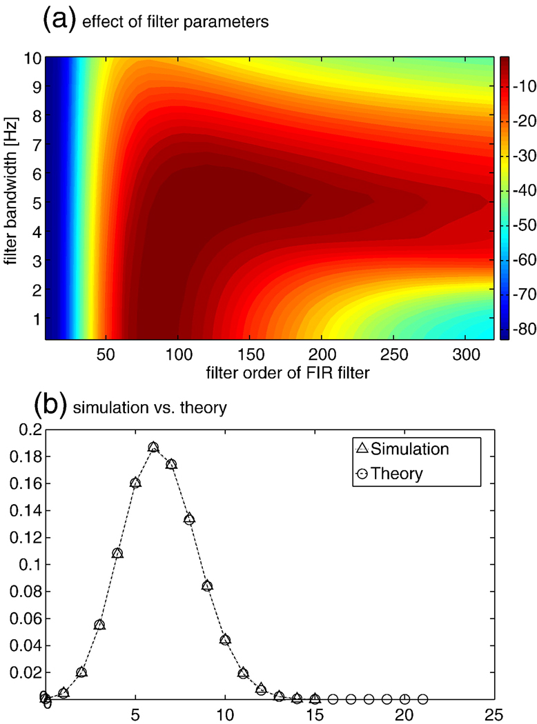
Typically, the bPLV is computed over a time range, covering some base line and some stimulus condition and the question of interest is, whether the synchronization index changed from not-synchronized, i.e. coming from the random phase distribution, to synchronized, and how significant this change is. If the baseline distribution follows the random phase distribution p(x,N), we can set a threshold x_T with the associated cumulative probability p_T = c(x_T,N) and test for the number of times q that x exceeds the threshold during the stimulus period. If the whole stimulus period contains k samples, then the distribution for q is given by the binomial distribution and the probability of finding q threshold crossings in k samples is F(q; k, p_T), the cumulative binomial distribution. However this is only true if the bPLV for each sample is independent from the next sample. This is not the case, when the bPLV is computed from bandpass-filtered data and is correlated in time due to the filter. Let us assume a discretely sampled signal x(t), where t is the discrete time index, with autocorrelation C(τ) = Σ_tx(t)x(t−τ) at lag τ, for which each sample is independent from the other samples, i.e. we have C(0) = c and C(τ) = 0 for τ ≠ 0. The filtered signal x_f will be $x_f(t)={\displaystyle {\sum }_{i=0}^{n}b(i)x(t-i)}$, where n is the filter order and b(i) are the filter coefficients. For the filtered signal, the autocorrelation will be $C_f(\tau )={\displaystyle {\sum }_{i=0}^n{\displaystyle {\sum }_{j=0}^{n}b(i)b(j)C(\tau -i+j)}}$ and consequently C_f(τ) ≠ 0 ∀ τ = j − i, the filtered signal will be correlated for all lags τ ≤ n and samples within this lag will not be independent any more. Also, for any lag τ > n the autocorrelation of the filtered signal will be 0. Independence of samples for the filtered signal can be achieved by considering only samples with a distance above the filter order, i.e. by down sampling the original filtered signal by k/(n + 2). Reducing the data by k/(n + 2) represents an upper limit because typically the coefficients of the filter will decay quickly and consequently down sampling by a factor smaller than n + 2 will still produce sufficiently uncorrelated samples of the bPLV. This imposes some limits on the signals that can be analyzed in this way, since it requires either the signal to have sufficient length to allow for meaningful down sampling or the filters to be sufficiently short, or conversely, the bandwidth across which synchronization is observed, has to be sufficiently wide. Since filter design depends on many factors, we will only briefly discuss the effect of the filter order and bandwidth on the bPLV for an ordinary hamming window based FIR bandpass filter, implementations of which can found e.g. in the Signal processing toolbox for Matlab (The Mathworks Inc., Natick MA, USA). The only variables for this filter are its order n and the width of the passband. The length of the hamming window for this filter is n + 1 and the magnitude at the center of the passband is scaled to one. We used the same simulated data as in the previous section on non-linearity to analyze the effect of the filter order and the bandwidth on the bPLV. The simulated data are bi-phase coupled in the interval [0,1]s and we computed the mean bPLV over this interval, varying the filter order from n = 8 to n = 320 and the bandwidth from 0.25 Hz to 10 Hz. We compute the relative change to the original simulation parameters, which used a filter order of n = 80 and a bandwidth of 2 Hz. The results of this simulation are shown in Fig. 4a, where the deviation of the mean bPLV over the [0,1]s interval from the original simulated bPLV is shown in percent. This figure shows that the quality of the bPLV estimation depends on both the bandwidth of the filter with respect to the original bandwidth at which the signals are coupled and on the proper filter order, which determines how sharp the magnitude/phase response falls off. If the synchronization bandwidth is larger than filter bandwidth, the choice of the filter order becomes critical, since higher orders of the filter will lead to a narrower magnitude/phase response and thus only parts of the original synchronized phases may be used in the bPLV computation. If the filter is either to wide, or has a too low order, its magnitude/phase response will lead to incorporation of non-synchronized phases in the bPLV and the estimate will be off the ‘true’ synchronization as well. Therefore it is important to note that the choice of filter parameters determines what bandwidth of synchronization can actually be observed. The choice of a filter order of n = 80 at a sampling rate of 250 Hz and a bandwidth of 2 Hz for our data analysis, leads to −5 dB attenuation at the band edges, i.e. +/− 1 Hz off the band center and to −60 dB suppression at +/− 2 Hz off the band center. Consequently, with these parameters, all synchronization measures have an accuracy of 4 Hz in frequency space. Fig. 4b shows the comparison between the theoretical cdf for the number of threshold crossings and the empirical cdf from a simulation. We simulated 40,000 bPLV time series from 200 signals with random phases to compute the bPLV and build the empirical distribution. Each time series was 1249 time samples long, and 30 trials per channel were simulated. We assumed a sampling rate of 250 Hz. A FIR filter of order 80 was used to filter the simulated signals at 13 Hz, 78 Hz and 91 Hz with a bandwidth of 2 Hz. The bPLV from f₁ = 13, f₂ = 78 Hz coupling to f₃ = 91 Hz was computed between all 200 signals. The resulting bPLV time series were down sampled by a factor of 60 to an effective number of 21 time samples. In our example, we set the threshold to a low value of 0.1, which leads to a probability of 0.74 per sample for the bPLV to exceed it, in order compare the theoretical and empirical cdf for a larger number of threshold crossings. The figure shows that simulation and theoretical prediction of the cdf are consistent.

Fig. 4.

(a) Effect of the filter parameters of the FIR filter on the estimate of the bPLV for simulated sources. The deviation of the simulated ‘true’ synchronization index is shown. The filter order is shown on the x-axis and the filter bandwidth on the y-axis. The signals were simulated using a filter order n = 80 and a bandwidth of 2 Hz. (b) Comparison of the theoretical cdf for finding q threshold crossings of the bPLV with a threshold of x_T = 0.1 in 1249 samples and a simulation. Circles show the cdf for the theoretical prediction; triangles show the results of the simulation.

Simulations: bPLV applied to EEG

Simulation setup

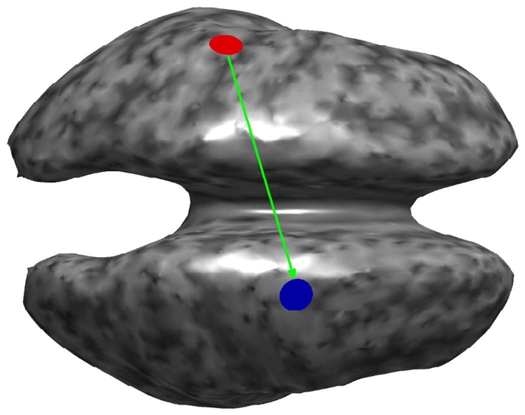
When the non-invasive methods EEG and MEG are used to record neuronal activity, the resulting map of this activity on the cortex, if an inverse method was used, or directly in electrode/sensor space is not as well resolved as ECoG and consequently, cross-talk has a significant effect on bPLV and PLV. The effect of this crosstalk is very sensitive to the location of the sources. It is also sensitive to the inverse method being used. It can depend on the particular head model. Here, we briefly discuss the effects of the inverse mapping on the bPLV. We used the Montreal Brain phantom (Collins et al., 1998) as realistic head model with four layers, skin, outer skull, CSF and white matter. We placed 64 electrodes, based on the extended 10–20 system (Oostenveld and Praamstra, 2001) on our model and computed an EEG forward model using the boundary element method. Sources in this model were constrained to lie on the white matter/cerebral cortex interface, which had 10,001 nodes. The forward model computation was carried out using the BrainStorm package (www.neuroimage.usc.edu/brainstorm). We assumed a common average reference for our forward model. Our simulation setup is schematically shown in Fig. 5, where we inflated the white matter/cerebral cortex interface for better visibility. Two sources, for which we simulated synchronized time courses, were placed onto the cortical surface, one on each hemisphere. We used the same time courses as described previously in the section on non-linearity as source time series, i.e. the red and the blue source in our simulation were biphase coupled in the interval (0 s to 1 s) with frequencies f₁ = 13, f₂ = 78 Hz in red coupling to f₃ = 91 Hz in blue. In a similar fashion, we simulated phase coupled sources at the same spatial location, with the coupling frequency at f = 91 Hz. The time course of the remaining sources was set to Gaussian white noise with amplitude at 0.1 times of the mean signal strength in order to simulate synchronized sources with a high signal-to-noise ratio. We used this source configuration to generate 46 trials of EEG data in 64 channels.

Fig. 5.

Simulation setup. The white matter/cerebral cortex interface was used as source space and two synchronized sources (red, blue disks) were used, one in each hemisphere. In case of the bPLV the direction of interaction (green arrow) was from red to blue. Note that the surface has been inflated for better visibility. The grey color scale was used to indicate the cortical curvature.

Simulation results

The simulated EEG trials were used to compute an inverse solution, where we used a linear minimum norm estimate with a regularization parameter λ equal to 10% of the largest eigenvalue of the leadfield matrix (Darvas et al., 2004). This type of inverse solution is commonly used with EEG or MEG recordings and has been used also in studies of cortical synchronization (Lin et al., 2004; Bar et al., 2006). A source time series for each trial and cortical node was computed and we computed the mean PLV and bPLV over the interval (0 s to 1 s) for each possible source pair. For comparison, the same computation was carried out over the interval (−1.5 s to −0.5 s), were the sources were not phase or biphase coupled.

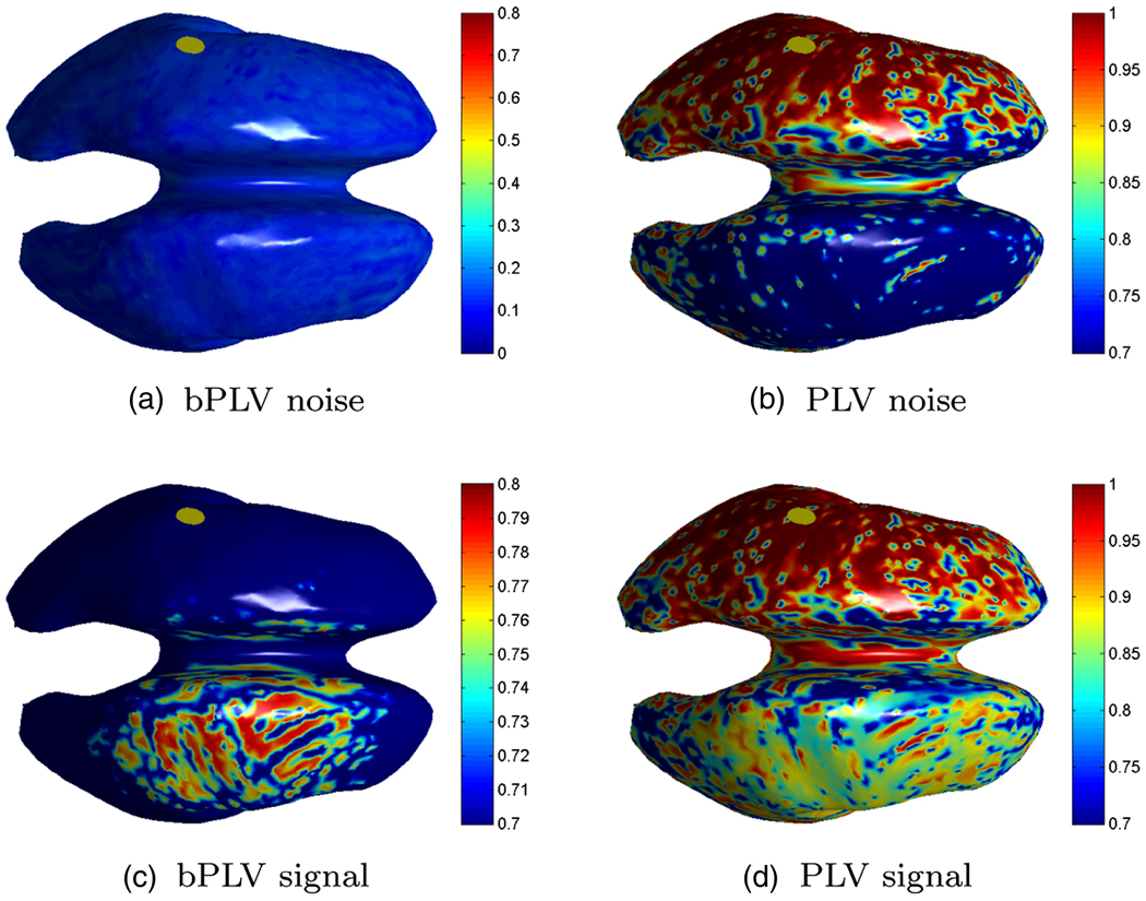
The results of this computation are shown in Fig. 6. We denote the left hemispheric source as ‘origin’ and the right hemispheric source as ‘target’. Here we assume, that the origin of the interaction is known and map only the bPLV/PLV values associated with this source, i.e. just a single row of the 10,001 × 10,001 interaction map. This particular row of the interaction map shows all cortical areas that are synchronous, as measured by either PLV or bPLV, with the origin. As expected, the cross talk effects for the bPLV are considerably lower compared to the PLV, since it is an asymmetric measure. During the noise period, the bPLV interaction map, shown in Fig. 6(a) does not show any significant synchronization with the origin. On the other hand, for the PLV, high synchronization in the vicinity of the origin is present even for the noise period due to volume conduction effects (Fig. 6(b)). When we compute the synchronization map during the period, where the two sources are synchronized, the bPLV map correctly shows increased synchronization between the origin and the right hemisphere only, whereas the PLV, due to crosstalk, shows increased synchronization in both hemispheres. The fact that the reconstruction of the target source is blurred in both cases results from the limited resolution of the inverse method, which produces crosstalk between cortical sites near the origin and the target. However, the bPLV is not sensitive to crosstalk of the origin with itself and thus shows, correctly, only synchronization with the target during the signal period. In essence, Fig. 6 is an anatomical representation of Fig. 3, where the ε parameter is now determined by anatomical location.

Fig. 6.

Mapping of the PLV/bPLV interaction of the left hemispheric source (see Fig. 5) to the right hemispheric source for the signal (0 s to 1 s) and noise or baseline period (−1.5 s to −0.5 s). The yellow disk indicates the position of the left source. Different scales were used to make the interaction mappings more visible.

A real world example: application to ECoG data

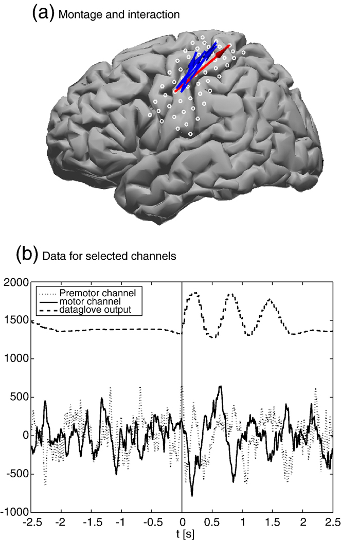
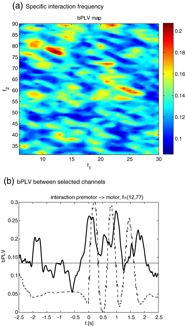
In a previous study, we found that for cued thumb movements, there is a movement specific increase of the bPLV between the α-rhythm (10–13 Hz) and the high γ band (77–81 Hz). This synchronization takes place at movement onset between a pre-motor and a motor area. A detailed description of the study and a discussion of its results can be found in Darvas et al. (2009). Here, we demonstrate our methods with a new data set that was recorded using the same paradigm. Notably, we use the random phase distribution assumption here to test for the significance of the results, rather than running computationally intensive permutation tests. Data was recorded with ECoG from 53 electrodes over the left hemisphere, covering the pre-motor and motor areas. The grid was implanted prior to surgery in a patient with epilepsy. The subject gave informed consent according to the protocol approved by the internal review board (IRB) of the University of Washington. The subject was visually cued to move the right thumb, and the actual movement was recorded with a data glove. Data was initially sampled at 1 kHZ and down sampled to 250 Hz during post processing. One channel, i.e. electrode 53, was noisy and excluded from further analysis. In order to reduce the impact of artifacts, the data was re-referenced to a common average reference. A total of N = 46 trials was recorded. We segmented the data based on the data glove, using the rising slope of the data glove output for thumb movement, where we set t=0. The montage for this subject and the mean time courses for the channels which we identified as candidates for increased bPLV (see Darvas et al., 2009) are shown in Fig. 7. We selected the interacting channel pair as the electrodes spatially closest to the mean interaction locations for which bPLV interaction already had been established. In order to find the precise interaction frequency pair, we scanned the potential interaction frequencies from 6 to 30 Hz and from 31 Hz to 90 Hz in 1 Hz steps. For each frequency pair, a bPLV time course was computed, where we used a bandpass FIR filter of order 80, that was applied forward and backward to remove phase distortions, with a bandwidth of 1 Hz. Since we cannot be certain about the exact temporal onset of the interaction, we computed the mean bPLV for each pair between −0.5 s and 1 s, assuming that any movement related increase should take place in that interval. The resulting values produce a frequency-by-frequency map, which shown in Fig. 8(a) This map shows the peak bPLV increase at (12,77) Hz. The smoothed time course of the bPLV for this frequency pair, along with the scaled data glove output, is shown in Fig. 8(b).

Fig. 7.

(a) The electrode placement for the subject in Talairach space, using a generic cortical surface, and the previously identified interaction sites during thumb movement. The blue arrows show interactions found in four other subjects, projected into the same coordinate system. The red arrow shows the interaction for the current study between a pre-motor and a motor region. (b) The average time course for these regions, along with the data glove output. The solid and dotted lines show the mean ECoG traces and the dashed line the mean data glove output. The bPLV interaction between these two channels cannot be readily seen in the time-domain.

Fig. 8.

(a) The frequency-by-frequency map for the mean bPLV increase for the pre-motor-motor channel pair. The peak of the bPLV is localized at (12,77) Hz. (b) The associated time course of the smoothed bPLV (solid line), along with the scaled data glove output (dashed line). There is a significant increase in bPLV coinciding with the actual finger movement as shown by the data glove. The mean bPLV for two random phase signals is also shown (horizontal line), which is well below the movement induced bPLV increase.

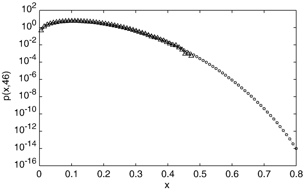
This example shows that there is a task related increase of the bPLV in this subject. In order to compute the significance of this bPLV increase, we first tested if the interaction bPLV in the pre-movement data across all channels is indeed a random phase interaction and our use of Eq. 2 as the null-distribution is justified. We define the pre-movement period from −2 s to −0.5 s. For 52 channels and 374 samples in the pre-movement segment we get 52² × 374 ≈ 10⁶ samples of bPLV values for the baseline. If we correct for potential temporal correlations by the filter order of 80, this number is reduced to ≈ 12000 samples, which is sufficient to build a histogram of the distribution of bPLV values for the baseline. Fig. 9 shows the comparison of p(x, 46) with the actual distribution of bPLV for the baseline. We used a log scale on the y-axis to emphasize the tail of the distribution. The actual distribution matches the theoretical distribution well, except for the very end of the tail, where we do not have enough samples in our data to accurately represent p(x,46). The good match of the measured baseline distribution with p(x,46) justifies our assumption that we can use p(x,46) and its associated cdf, c(x,46), in our calculations. If we set our threshold at a p-value of 0.05 for an individual realization of the bPLV during finger movement, then we find the threshold for the bPLV=0.2545. We computed the bPLV time series for each of the 52² possible channel interactions between 12 and 77 Hz. Since we only have 374 samples in our movement segment (−0.5 s to 1 s) and pre-movement segment (−2 s to −0.5 s), we down sampled the bPLV time series only by a factor 30, which yields 13 independent time samples of the bPLV per segment, and count the threshold crossings during finger movement and during rest for each channel pair. Under the null-hypothesis of random phases, i.e., no interaction of the channels during movement, the distribution of the number of threshold crossings q for the threshold of bPLV=0.2545 will be given by F(q;13,0.05). For the selected pre-motor to motor interaction channel pair, we find a total of 5 threshold crossings during the movement period of 13 samples' length, which corresponds to a likelihood of p=3*10⁻⁴. For the same channel pair, we find just 1 threshold crossing in the pre-movement period, corresponding to p = 0.86 (for getting 1 or less under the null hypothesis for the baseline as opposed to p=3*10⁻⁴ of finding 5 or more threshold crossings during movement).

Fig. 9.

Comparison of the theoretical pdf of the bPLV based on Eq.2 and the distribution of the bPLV between all channel pairs for the premovement segment. Circles show the theoretical prediction; triangles show the results of the actual data. Note that a log scale is used on the y-axis. The curves match well, which implies that the bPLV between most cortical regions adheres to the random phase distribution. This justifies the use of the theoretical distribution as a baseline

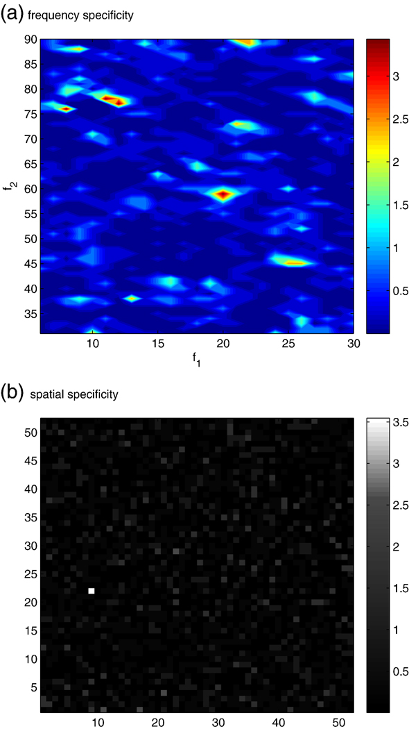
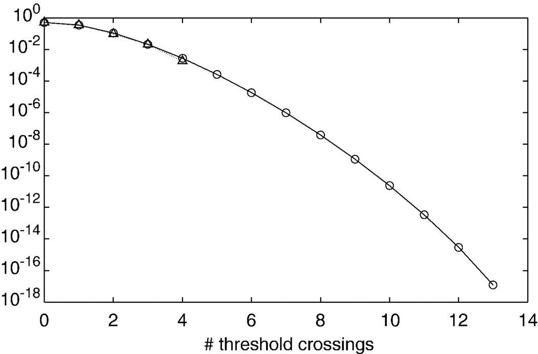
We summarize our findings in Fig. 11. We find that the measured distribution of threshold crossings during the rest period across all channels pairs, when down sampling in time by a factor of 30, matches the theoretical distribution well (see Fig. 10). This justifies our use of the binomial cdf F(q;13,0.05) to compute p-values for our measured bPLV threshold crossings. Fig. 11 shows the p-value maps for the specifically selected channel pair (pre-motor to motor) for a range of interaction frequencies (6–30,31–90) Hz, as well as for a specific interaction frequency (12,77) Hz across all channel pairs. We find for the specific frequency/channel pair, that p=3*10⁻⁴ is the lowest p-value across all channels for the (12,77) Hz frequency interaction and that for this channel pair (at position (22,9) in Fig. 11(b)), this frequency pair has also the lowest p-value, thus confirming our initial assumption, that there is a significant increase in bPLV during finger movement between these two pre-motor and motor electrode sites at α and high γ frequencies. Using the trial-shuffling permutation test, we also find that based on 10⁵ permutations of the trial order in the movement segments, p=5*10⁻⁴, indicating that the observed synchronization is genuine.

Fig. 11.

(a) The frequency-by-frequency map of the p-values of the threshold crossings for the selected pre-motor to motor interaction. A negative log scale was used (base 10). (b) The channel by channel p-value map of the threshold crossings during movement for the bPLV interaction at (12,77) Hz. The coordinates of the selected channels in pre-motor and motor cortex are (9,22), where the map shows the lowest p-value. A negative log scale was used. This shows that the observed bPLV coupling is specific in space, i.e. the selected electrode pair, and frequency.

Fig. 10.

The theoretical pdf for the number of threshold crossings. Circles indicate the theoretical pdf (solid line) and triangles the estimated pdf from the data (dotted line). A log scale on the y-axis was used. The good match between the theoretical pdf and the data justifies using the theoretical result as the baseline.

Discussion and conclusion

The bPLV measure can be used to detect non-linear synchronization between three different frequencies, which adds another dimension to the space of cortical interactions. Instead of interactions limited to a single frequency we can now look for interactions across the (f₁,f₂) frequency map. In combination with the already large number of possible interactions across detectors/source nodes, this poses a serious detection problem as we are looking for task related changes of the synchronization measure in the 4D space spanned by all possible channel and frequency pairs. In our real world example there were 52 channels and 1500 frequency pairs, leading to 405,6000 bPLV time series to explore. Using a priori knowledge to limit this number, e.g. using specific information about the location of the interaction and the involved frequencies, as we did in our example, is one obvious way to address this problem.

Our experimental ECoG data have shown, that the bPLV for most interactions between channel pairs can be described by the random phase statistic, independent of movement or rest, which demonstrates a useful property of the phase-locking synchronization measures: The presence of synchronization can be detected based on an absolute null-hypothesis, i.e. random phases, for which a closed form solution for the pdf and cdf exists. Since detection of phase synchrony does not require a baseline, it can also be applied to spontaneous activity, which has potential utility for BCI (Brain Computer Interface) applications. It should be noted however, that the random phase distribution cannot distinguish between functional synchronization and volume conduction effects and it is therefore essential, that the signals are free of such effects, when testing for synchronization. When synchronization measures are used in exploratory way, it is essential to apply appropriate multiple comparison corrections to avoid spurious detections, which in turn require precise knowledge of the distribution of the synchronization measure under the null hypothesis. For measures that are affected by the signal amplitude, e.g. coherence or bi-coherence, the baseline amplitude distribution of the involved cortical regions has to be determined empirically. While this can be done through resampling techniques, e.g. permutation tests or bootstrapping, it is computationally intensive when a larger number of interactions are considered as in our example given above. Here again the phase-based methods have the advantage of an absolute null-hypothesis, i.e. the random phase distribution, that allows us a precise computation of p-values without resampling. While we found for our ECoG example, that the baseline in this case indeed follows this distribution, it is essential to test this assumption for individual data analysis.

It is important to note that bPLV and PLV are complementary methods, as they measure different types of synchronization, single frequency synchronization, including synchronizations of harmonics of this frequency, in case of the PLV and unlimited frequency-to-frequency synchronization in case of the bPLV. Neither method can substitute for the other, since bPLV is blind to single frequency interactions, while PLV cannot detect cross-frequency interaction, except for harmonic couplings. Our comparison between the two modalities shows however, that, if interactions exist that can be detected by bPLV, they are easier to identify and less prone to suffer from cross-talk. For symmetric measures, such as the PLV or coherence, the crosstalk problem can be addressed by contrasting the signal with a baseline, since the crosstalk effects are of purely geometrical nature and can be expected to be the same for the baseline as for the signal. If a sufficiently large baseline segment is available, one can compute for example a Z-score for the PLV values, where the mean baseline PLV for each time series is subtracted from the signal PLV and the resulting difference is normalized by the baseline standard deviation (Bar et al., 2006). However such a baseline-signal comparison will only work well, if the contrast between baseline and signal is sufficiently large. If the sources of interest are geometrically close and the crosstalk between them raises the synchronization baseline toward 1 due to volume conduction, functional synchronization effects are diminished and might become undetectable.

References

- Ahissar E, Kleinfeld D. Closed-loop neuronal computations: focus an vibrissa somatosensation in rat. Cereb. Cortex. 2002;13:53–62. doi: 10.1093/cercor/13.1.53. [DOI] [PubMed] [Google Scholar]
- Bar M, Kassam K, Ghuman A, Boyshan J, Schmid A, Dale A, Hämäläinen M, Marinkovic K, Schacter D, Rosen B, Halgren E. Top-down facilitation of visual recognition. Proc. Natl. Acad. Sci. 2006;103(2):449–454. doi: 10.1073/pnas.0507062103. [DOI] [PMC free article] [PubMed] [Google Scholar]
- Canolty R, Edwards E, Dalal S, Soltani M, Nagarajan S, Kirsch H, Berger M, Barbaro N, Knight R. High gamma power is phase-locked to theta oscillations in humans neocortex. Science. 2006;313:1626–1628. doi: 10.1126/science.1128115. [DOI] [PMC free article] [PubMed] [Google Scholar]
- Collins D, Zijdenbos A, Kollokian V, Sled J, Kabani N, Holmes C, Evans A. Design and construction of a realistic digital brain phantom. IEEE Trans. Med. Imag. 1998;17:463–468. doi: 10.1109/42.712135. [DOI] [PubMed] [Google Scholar]
- Darvas F, Pantazis D, Kucukaltun-Yildirm E, Leahy R. Mapping human brain function with MEG and EEG: methods and validation. NeuroImage. 2004;23:S289–S299. doi: 10.1016/j.neuroimage.2004.07.014. [DOI] [PubMed] [Google Scholar]
- Darvas F, Miller K, Rao R, Ojemann J. Non-linear phase-phase coupling mediates communication between distant sites in human neocortex. J. Neurosci. 2009;29(2):425–434. doi: 10.1523/JNEUROSCI.3688-08.2009. [DOI] [PMC free article] [PubMed] [Google Scholar]
- Gabbiani F, Krapp H, Koch C, Laurent G. Multiplicative computation in a visual neuron sensitive to looming. Nature. 2002;420(21):320–324. doi: 10.1038/nature01190. [DOI] [PubMed] [Google Scholar]
- Granger C. Investigating causal relations by econometric models and cross-spectral methods. Econometrica. 1969;37:424–438. [Google Scholar]
- Gross J, Kujala J, Hamalainen M, Timmermann L, Schnitzler A, Salmelin R. Dynamic imaging of coherent sources: studying neural interactions in the human brain. Proc. Natl. Acad. Sci. 2001;98(2):694–699. doi: 10.1073/pnas.98.2.694. [DOI] [PMC free article] [PubMed] [Google Scholar]
- Hughes B. Random Walks and Random Environments. Vol. 1. Random Walks: Clarendon Press; 1995. [Google Scholar]
- Hurtado J, Rubichinsky L, Sigvardt K. Statistical method for detection of phase-locking episodes in neural oscillations. J. Neurophysiol. 2004;91(4):1883–1898. doi: 10.1152/jn.00853.2003. [DOI] [PubMed] [Google Scholar]
- Kahana M. The cognitive correlates of human brain oscillations. J. Neurosci. 2006;26(6):1669–1672. doi: 10.1523/JNEUROSCI.3737-05c.2006. [DOI] [PMC free article] [PubMed] [Google Scholar]
- Lachaux J, Rodriguez E, Martinerie J, Varela F. Measuring phase synchrony in brain signals. Hum. Brain Mapp. 1999;8:194–208. doi: 10.1002/(SICI)1097-0193(1999)8:4<194::AID-HBM4>3.0.CO;2-C. [DOI] [PMC free article] [PubMed] [Google Scholar]
- Lachaux J, Lutz A, Rudrauf D, Cosmelli D, Le Van Quyen M, Martinerie J, Varela F. Estimating the time-course of coherence between single-trial brain signals: an introduction to wavelet coherence. Clin. Neurophysiol. 2002;32(3):157–174. doi: 10.1016/s0987-7053(02)00301-5. [DOI] [PubMed] [Google Scholar]
- Le Van Quyen M, Foucher J, Lauchaux J, Rodriguez E, Lutz A, Martinerie J, Varela F. Comparison of hilbert transform and wavelet methods for the analysis of neuronal synchrony. J. Neurosci. Methods. 2001;111:83–89. doi: 10.1016/s0165-0270(01)00372-7. [DOI] [PubMed] [Google Scholar]
- Lin F, Witzel T, Hämäläinen M, Dale A, Belliveau J, Stufflebeam S. Spectral spatiotemporal imaging of cortical oscillations and interactions in the human brain. NeuroImage. 2004;23(2):582–595. doi: 10.1016/j.neuroimage.2004.04.027. [DOI] [PMC free article] [PubMed] [Google Scholar]
- Miller K, Makeig S, Hebb A, Rao R, denNijs M, Ojemann J. Cortical electrode localization from X-rays and simple mapping for electrocorticographic research: the “Location on Cortex” (LOC) package for MATLAB. J. Neurosci. Methods. 2007;162:303–308. doi: 10.1016/j.jneumeth.2007.01.019. [DOI] [PubMed] [Google Scholar]
- Nikias C, Mendel J. Signal processing with higher-order spectra. IEEE Signal Process. Magazine. 1993;10(3):10–37. [Google Scholar]
- Oostenveld R, Praamstra P. The five percent electrode system for high-resolution EEG and ERP measurements. Clin. Neurophysiol. 2001;112:713–719. doi: 10.1016/s1388-2457(00)00527-7. [DOI] [PubMed] [Google Scholar]
- Palva S, Palva J. New vistas for α-frequency band oscillations. Trends Neurosci. 2007;30(5):150–158. doi: 10.1016/j.tins.2007.02.001. [DOI] [PubMed] [Google Scholar]
- Pantazis D, Nichols T, Baillet S, Leahy R. A comparison of random field theory and permutation methods for the statistical analysis of MEG data. NeuroImage. 2005;25:383–394. doi: 10.1016/j.neuroimage.2004.09.040. [DOI] [PubMed] [Google Scholar]
- Rudrauf D, Douiri A, Kovach C, Lauchaux J, Cosmelli D, Chavez M, Adam C, Renault B, Martinerie J, Le Van Quyen M. Frequency flows and the time-frequency dynamics of multivariate phase synchronizations in brain signals. NeuroImage. 2006;31:209–227. doi: 10.1016/j.neuroimage.2005.11.021. [DOI] [PubMed] [Google Scholar]
- Schack B, Vath N, Petsche H, Geissler H, Moeller E. Phase-coupling of theta-gamma EEG rythms during short-term memory processing. Int. J. Psychophysiol. 2002;44:143–163. doi: 10.1016/s0167-8760(01)00199-4. [DOI] [PubMed] [Google Scholar]
- Shils J, Litt M, Skolnick B, Stecker M. Bispectral analysis of visual interactions in humans. Electroencephalogr. Clin. Neurophysiol. 1996;98:113–125. doi: 10.1016/0013-4694(95)00230-8. [DOI] [PubMed] [Google Scholar]
- Singer W. Synchronization of cortical activity and its putative role in information processing and learning. Annu. Rev. Phsyiol. 1993;55:349–374. doi: 10.1146/annurev.ph.55.030193.002025. [DOI] [PubMed] [Google Scholar]
- Tass P, Rosenblum M, Weule J, Kurths J, Pikovsky A, Volkmann J, Schnitzler A, Freund H. Detection of n:m phase locking from noisy data: application to magnetoencephalography. Phys. Rev. Lett. 1998;81(15):3291–3294. [Google Scholar]