Level-set algorithm for the reconstruction of functional activation in near-infrared spectroscopic imaging

Abstract

We introduce a new algorithm for the reconstruction of functional brain activations from near-infrared spectroscopic imaging (NIRSI) data. While NIRSI offers remarkable biochemical specificity, the attainable spatial resolution with this technique is rather limited, mainly due to the highly scattering nature of brain tissue and the low number of measurement channels. Our approach exploits the support-limited (spatially concentrated) nature of the activations to make the reconstruction problem well-posed. The new algorithm considers both the support and the function values of the activations as unknowns and estimates them from the data. The support of the activations is represented using a level-set scheme. We use a two-step alternating iterative scheme to solve for the activations. Since our approach uses the inherent nature of functional activations to make the problem well-posed, it provides reconstructions with better spatial resolution, fewer artifacts, and is more robust to noise than existing techniques. Numerical simulations and experimental data indicate a significant improvement in the quality (resolution and robustness to noise) over standard techniques such as truncated conjugate gradients (TCG) and simultaneous iterative reconstruction technique (SIRT) algorithms. Furthermore, results on experimental data obtained from simultaneous functional magnetic resonance imaging (fMRI) and optical measurements show much closer agreement of the optical reconstruction using the new approach with fMRI images than TCG and SIRT.

1 Introduction

Near-infrared spectroscopic imaging (NIRSI) is an emerging technique, based on the propagation of light through tissue:^1–3 Owing to its sensitivity to oxy- and deoxyhemoglobin concentrations and high temporal resolution, this approach offers considerable promise in functional brain studies.^4–7 Moreover, its ability to measure the changes in the optical scattering properties of activated neurons makes it even more attractive.⁸ However, the main drawback of this technique is the poor spatial resolution, mainly due to the diffuse nature of light propagation, the low number of source detector pairs, and the limited penetration of light into the brain (due to the highly scattering nature of tissue).⁹

A popular forward model in NIRSI is the diffusion equation, derived as an approximation to the radiative transfer equation (RTE). Because this problem is nonlinear with respect to the unknown parameters (absorption and scattering coefficients), nonlinear reconstruction schemes including iterative perturbation methods^2,10,11 and back-propagation techniques^12,13 have been proposed to solve this problem. These approaches make few assumptions about the forward problem and the medium. However, they are computationally expensive and require sophisticated techniques to ensure convergence. Our focus is on functional imaging, where the objective is to measure the perturbations in the absorption coefficient of the brain tissue as a function of the stimulus.^5,7 The general approach in this setup is to linearize the forward problem using the Born or Rytov approximation, assuming the perturbation in the absorption coefficient to be small. This approximation reduces the problem to the well-studied class of linear inverse problems.¹⁴ Classical techniques such as algebraic methods,^15,16 Tikhonov regularized reconstructions,¹⁷ and subspace methods¹⁵ are the currently used schemes. Recently, several authors have reported approaches to constrain the reconstructions using priors from alternate modalities such as functional magnetic resonance imaging (fMRI) and structural MR scans.^16,18–21

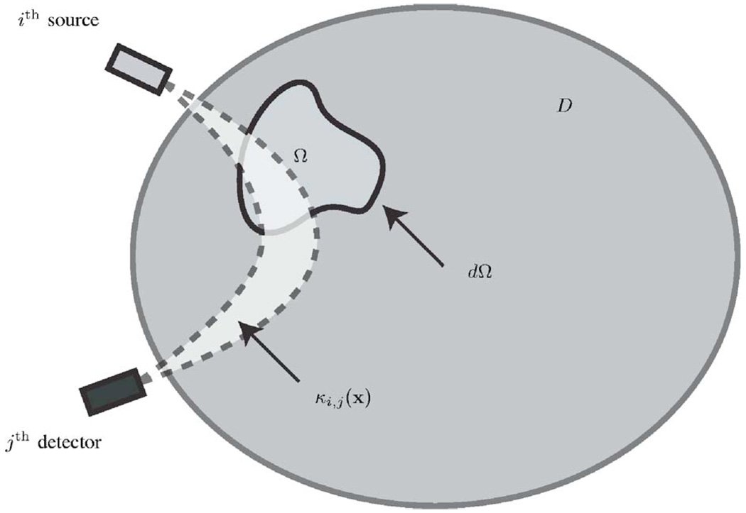
The main focus of this paper is to improve the spatial resolution of the reconstructions by using a better reconstruction algorithm. Our approach is based on the assumption that the activations are spatially concentrated or sparse; in other words, only a subregion of the brain is activated at any instant. With this assumption, the reconstruction can be posed as a sparse inverse problem.^22–24 Theoretical results indicate that if a signal is sparse, it can still be recovered from an underdetermined system of equations, provided the number of unknowns is lower than the number of independent measurements. Because the number of independent measurements in NIRSI is often much smaller than the number of activated voxels, we propose to enforce additional constraints such as the activation pattern being smooth over the region (see Fig. 1 for an illustration) to further reduce the degrees of freedom. In traditional approaches, such as subspace methods or truncated conjugate gradients (TCG) algorithm, the reconstruction is regularized by restricting the solution to a low-dimensional eigenspace of the system matrix. This space, in general, need not represent the class of natural images and hence may result in artifacts as shown later. In contrast, the new method introduces penalties for deviation of the estimate from the expected natural image characteristics to obtain well-posed reconstructions.

Fig. 1.

The setup of the reconstruction algorithm illustrated in two dimensions. Ω denotes the region of activation (where the function f is assumed to be nonzero). dΩ is the boundary of Ω. D denotes the mask corresponding to the brain (it can also be defined as a subregion of the brain where the light bundles have significant amplitude). κ_i,j (x) is the light bundle between the ith source and the jth detector. With this assumption of f being zero in D\Ω, the forward model can be formulated as Eq. (9).

The standard l₁ minimization approach to sparse problems^23,24 does not offer a convenient way to account for the additional properties of brain activations. Instead, we propose a new algorithm based on variational principles that is an extension of Ref. 25. We consider (a) the support of the activated regions (regions where the activations are nonzero) and (b) the value of the activations over this support as unknowns and solve for them using an iterative alternating two-step minimization of a cost function. In the first step, we assume an initial support from the previous iteration and solve for the activations over this region using the CG optimization algorithm. This step is similar in concept to Ref. 18, where the support is obtained from prior knowledge. In the next step, we evolve the support so as to minimize the cost function. This approach is similar in principle to Refs. ^26–28. We represent the support using the level-set formalism;²⁹ the evolution of the support can be posed as a simple partial differential equation, thanks to the well-developed level-set theory.^29,30 The two-step algorithm is iterated until convergence.

We used a Monte Carlo method to simulate light transport in a realistic head model and thus determine the light bundles and the perturbed optical signal. We perform quantitative and qualitative comparison of the proposed algorithm to the standard approaches, such as simultaneous iterative reconstruction technique (SIRT) and TCG. We also studied the performance of the algorithm to experimental data obtained from simultaneous fMRI and optical measurements.

2 Methods

In this section, we formulate the forward problem, discuss the simulation setup, and propose the new reconstruction algorithm.

2.1 Formulation of the Forward Problem

In this paper, we assume frequency-resolved measurements; the light sources are amplitude modulated by a sinusoid of a specified frequency ν. Although we focus on this setup, the proposed algorithm is general enough to accommodate time-resolved and continuous-wave measurements (with an appropriate change in forward model). The widely used forward model for the photon fluence in a highly scattering medium is the Helmholtz frequency-domain diffusion equation^4,15,31

$$[{\mathbf{\nabla }}^2+\frac{j\omega -c{\mu }_a(\mathbf{x})}{D}]\varphi (\mathbf{x})=-\frac{c}{D}q(\mathbf{x}).$$ (1)

Here ω =2πν, φ(x) is the photon fluence at the specified location x; μ_a(x) is the absorbtion coefficient; c is the velocity of light in the medium; and D = c/3μ′_s is the diffusion coefficient. μ′_s is the reduced scattering coefficient and q(x) is the light source. This equation is obtained by approximating the general RTE, assuming that μ_s is not spatially varying (i.e., ‖∇μ_s‖→0).

Functional activations give rise to small perturbations in μ_a(x) due to changes in local oxy- and deoxyhemoglobin concentrations. Denoting the perturbations in the absorption coefficient and the corresponding perturbation in the fluence as Δμ_a(x) and Δφ(x), respectively, and by assuming‖Δφ‖≪‖φ‖, we obtain

$$[{\mathbf{\nabla }}^2+\frac{j\omega -c{\mu }_a(\mathbf{x})}{D}]\mathbf{\Delta }\varphi (\mathbf{x})=-\frac{c}{D}\mathbf{\Delta }{\mu }_a(\mathbf{x})\varphi (\mathbf{x}).$$ (2)

Note that the above differential equation is linear inΔφ; it can be solved in terms of the corresponding Green’s function G(x,x′)

$$\mathbf{\Delta }\varphi (\mathbf{x})={\displaystyle {\int }_{{ℝ}^3}\underset{\kappa (\mathbf{x},\mathbf{x}\prime )}{\underbrace{-\frac{c}{D}G(\mathbf{x},\mathbf{x}\prime )\varphi (\mathbf{x}\prime )}}\mathbf{\Delta }{\mu }_a(\mathbf{x}\prime )\mathrm{d}\mathbf{x}\prime .}$$ (3)

Hence, the perturbation in the fluence at a specified detector location x_j, corresponding to a source located at x_i [specified by the corresponding baseline fluence distribution φ_i (x)], is given by

$$\mathbf{\Delta }\varphi (i,j)\mathbf{\Delta }{\varphi }_i({\mathbf{x}}_j)={\displaystyle {\int }_{{ℝ}^3}{\mathbf{\kappa }}_{l,m}(\mathbf{x})\mathbf{\Delta }{\mu }_a(\mathbf{x})\mathrm{d}\mathbf{x},}$$ (4)

where the three-dimensional sensitivity function κ _i,j(x) = −c/D × G(x,x_j)φ _i(x) is termed as the light bundle between the ith source and jth detector. Note that the above equation indicates a linear relationship between the perturbation in the absorption coefficient and that of the optical signal.

2.2 Noise Process

It is experimentally observed that the noise at the jth detector due to the ith source [defined by η(i,j)] follows a Gaussian process with zero mean and standard deviation proportional to the amplitude of the corresponding baseline signal φ _i,j. (We assume source-detector distances of about 25 to 30 mm, including the biological noise contribution.) Collecting the measurements corresponding to the different source-detector pairs into a single vector, and denoting f(x) = Δμ_a(x), we obtain

$$\mathbf{y}={\displaystyle {\int }_{{ℝ}^3}\mathit{\kappa }(\mathbf{x})f(\mathbf{x})\mathrm{d}\mathbf{x}+\eta \text{.}}$$ (5)

Here

$$\mathbf{y}={[y(0,0),y(0,1)\dots y(M-1,N-1)]}^T,$$ (6)

$$\mathit{\kappa }(\mathbf{x})={[{\kappa }_{0,0}(\mathbf{x}),{\kappa }_{0,1}(\mathbf{x})\dots {\kappa }_{M-1,N-1}(\mathbf{x})]}^T.$$ (7)

2.3 Simulation of the Forward Problem

We use Monte Carlo simulations of the optical transport problem, discussed in Refs. ¹⁶ and ³², to generate the frequency-domain light bundles. The modulation frequency ν is chosen as 200 MHz. To generate realistic simulations, we use the segmentation of a magnetization-prepared rapid acquisition gradient echo (MP-RAGE) MRI brain scan along with scattering and absorbtion coefficients from Ref. 32 to obtain the light bundles. We insert a small bloblike perturbation (see Fig. 3) on the cortical region (10% of the nonstimulated absorption coefficient) and obtain the corresponding perturbed fluence measurements. We refer to the bloblike perturbation in the absorption coefficient as f_orig and the corresponding optical perturbation as y_orig.

Fig. 3.

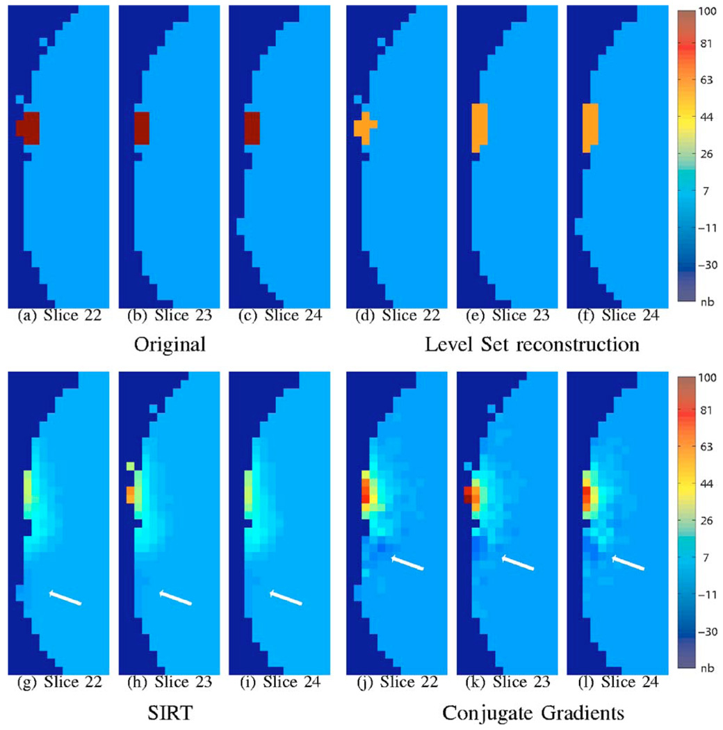
Reconstruction in the absence of noise. The range of the original signal is scaled to be in the range 0 to 100; the same scale factor is applied to the reconstructions. The voxel dimensions in the above figure are 4 mm³. The reconstructions are constrained to the brain (gray matter and white matter) and are displayed over the mask of the brain (gray matter and white matter). The nonbrain regions are marked as “nb” in the color bar. The top row consists of three slices of the original and level-set reconstructions each. Note that the level-set reconstructions are in close agreement with the original object. The corresponding slices of the reconstructions with SIRT and CG are displayed on the bottom row. Note that these reconstructions are distributed over a larger region and are oscillatory. The white arrows correspond to regions with negative amplitude. This effect is predominantly visible in the CG reconstructions. We used 64 iterations of CG and 400 iterations of SIRT. For the new algorithm, we used μ = 2e−3, ζ =0.2, λ=0.6.

Based on previous experimental results, we set the standard deviation of the noise process to be 2% of the baseline signal. Because the perturbation in the optical signal due to functional activation is often much smaller in amplitude as compared to the baseline, this corresponds to a very noisy scenario [the signal to noise ratio (SNR) of the perturbation signal is approximately −15 dB]. At such a high noise level, it is difficult to obtain reasonable reconstructions. Hence, it is common practice to average 𝒩 successive measurements to improve the SNR. With 𝒩 averages, the standard deviation of the noise process will decrease by a factor of $\sqrt{N}$ . In our experimental setup,^16,33 we time-domain multiplex the signals from individual channels and hence the time resolution is 20 ms per channel: we typically use around 50 to 100 averages; the resulting temporal resolution is still sufficient for hemodynamic studies.

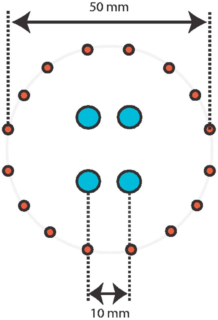
We assumed the source-detector configuration in Ref. 16 for the simulations (see Fig. 2). We denote the noise corrupted version of y_orig as y_measured. We then use the reconstruction algorithms to obtain the estimate of the signal (denoted by f̂) from y_measured.

Fig. 2.

Schematic of the optical probe: 16 sources arranged in a circular pattern and 4 detectors in the center used to obtain 64 source-detector pairs.

2.4 Reconstruction

By collecting the voxel values of f(x) into a vector f, the forward model ((9)) can be expressed as a matrix equation y = Af + η. Each voxel in the reconstructed image would correspond to a column of A. Similarly, a measurement corresponds to a row in A. In the context of sparse sampling, it is shown that if the submatrix of A, obtained by selecting any of its M columns is invertible, an activation pattern with M active voxels can be uniquely reconstructed with probability 1.³⁴ Unfortunately, the value of M, for which the condition number of all M column submatrices of A is reasonably low (well-conditioned matrix is required to ensure robust reconstructions in the presence of noise), is fairly small for the NIRSI forward model (M ≤ 16). Hence, we have to enforce additional constraints that are relevant to the functional imaging context (e.g., the activation pattern being smooth in the region of support, the boundary of the activations being smooth) to further reduce the degrees of freedom. We would now be searching for an activation pattern in the class of reconstructions that satisfy these constraints; we hypothesize that these constraints ensure a reasonably well-conditioned inversion problem.

The standard l₁ minimization approach to sparse problems^23,24 does not offer a convenient way to account for the additional properties of brain activations. Instead, we propose an alternate algorithm using variational principles. Assuming the activations to be support limited to subregions of the brain specified by Ω⊆D (see Fig. 1), we rewrite the forward model as

$$\mathbf{y}={\displaystyle {\int }_{\mathrm{\Omega }}\mathit{\kappa }(\mathbf{x})f(\mathbf{x})\mathrm{d}\mathbf{x}}+\mathit{\eta }.$$ (8)

The above expression can also be represented as

$$\mathbf{y}={\mathbf{\Lambda }}_{\mathrm{\Omega }}f+\mathit{\eta },$$ (9)

where Λ_Ω denotes the linear integral operator describing the measurement process. In practical implementations, the function values of f are vectorized. In this case, the operator Λ_Ω simplifies to a matrix.

Note that f and its support Ω in (9) are unknowns. We pose the estimation of these quantities as a numerical optimization problem; we define the cost function as

$$\begin{array}{cc}𝒞(f,\mathrm{\Omega })=\hfill & \underset{\text{data consistency}}{\underbrace{\Vert \mathbf{y}-{\mathbf{\Lambda }}_{\mathrm{\Omega }}f{\Vert }_w^2}}+\underset{\text{amplitude penalty}}{\underbrace{\mu {\displaystyle {\int }_{\mathrm{\Omega }}|f{|}^2\mathrm{d}\mathbf{x}}}}\hfill \\ \hfill & +\underset{\text{smoothness penalty}}{\underbrace{\mathrm{\lambda }{\displaystyle {\int }_{\mathrm{\Omega }}|\mathbf{\nabla }f{|}^2\mathrm{d}\mathbf{x}}}}+\underset{\text{volume penalty}}{\underbrace{\zeta {\displaystyle {\int }_{\mathrm{\Omega }}\mathrm{\text{dx}}}}}.\hfill \end{array}$$ (10)

The first term in Eq. (10) is a measure of the data consistency. ‖…‖ _w denotes the weighted l₂ norm

$$\Vert \mathbf{y}{\Vert }_{\mathbf{w}}^2={\displaystyle \sum _i{w}_i^2|y(i){|}^2.}$$ (11)

We choose the weight vector $\mathbf{w}=1/\sqrt{\left|\mathbf{\gamma }\right|}$ , where γ is the vector corresponding to the baseline signal. This is to account for the statistics of the noise. (The measurement with the largest noise variance gets the lowest weight, thus whitening the noise process.) The weighted norm can be converted to a simple l₂ norm by assuming the measurements as y′ = Wy, and ${\mathbf{\Lambda }}_{\mathrm{\Omega }}^{\prime }=\mathbf{W}{\mathbf{\Lambda }}_{\mathrm{\Omega }}$ , where W = diag(w_i); W is a diagonal matrix with the diagonal entries specified by the vector w. In the rest of this paper, we assume these modified quantities. However, for simplicity of notation, we will denote y′ and ${\mathbf{\Lambda }}_{\mathrm{\Omega }}^{\prime }$ by y and Λ_Ω, respectively.

The second and third terms in Eq. (10) are similar to the standard Tikhonov regularization terms used in inverse problems to make the inverse problem well-posed.¹⁴ The important difference with the standard setting is that these integrals are evaluated over Ω as compared to ℝ³ (the entire volume) in the standard scheme. This restriction ensures that we would not be smoothing across the boundaries between the activated and the nonactivated regions, thus avoiding the blurring of the edges of the activation regions. The second term penalizes the amplitude of the reconstructions, thus eliminating reconstructions with high amplitudes. The third term imposes a penalty on the roughness of f on its support. If λ →, ∞, ∇f would only be supported on dΩ, the boundary of Ω; we would be reconstructing a piecewise-constant function f. The last term in Eq. (10) constrains the volume of the activations; it ensures that the estimation of the support Ω is well-posed. The parameters λ, μ, and ζ control the strength of the additional penalties relative to the data consistency term. Note that in the absence of the second and third terms, the cost function is simply an l₀ minimization problem; one tries to find an f with the smallest possible support.

This approach of simultaneously estimating Ω and the function values is an extension of Ref. 25 to three dimensions. This approach is also conceptually similar to Refs. ²⁶ and ^35–38. A similar shape-based approach was used in the context of diffuse optical imaging in Ref. 39. They modeled the shape of the activation as an ellipsoid while the function values inside and outside the activation are approximated by harmonics. Our approach is more general because it can account for perturbations of arbitrary shape and topology. Moreover, we model the function values as arbitrary smooth functions.

The main difference between the new method and the one in Ref. 25 is the inclusion of additional Tikhonov regularization terms. In addition, the last term in Eq. (10) is also different from Ref. 25; we minimize the volume of Ω rather than the surface area of the boundary dΩ. The main reason to change this term is to improve the numerical stability of the algorithm. The functional activations typically occupy a very small region of space (≈ 10 to 15 voxels). Hence, the approximation of the curvature term using simple finite difference operators is not good enough for this application. Further-more, the new term minimizes the volume of the support that is desirable to ensure sparse reconstructions.

2.5 Algorithm

In Sec. 2.4, we have seen that the reconstruction of the activation pattern involves the minimization of Eq. (10)

$$f^{*}=\text{arg}\underset{f,\mathrm{\Omega }}{\text{min}}𝒞(f,\mathbf{\Omega }).$$ (12)

We use a two-step alternating minimization algorithm for this purpose.

2.5.1 Optimization scheme

In the first step, we estimate the optimal f, assuming Ω to be known. In the next step, we update Ω, assuming the value of f from the previous iteration. These steps are elaborated below.

1. Derivation of optimal f given Ω

The derivation of optimal f given Ω can be formulated as

$$f^{*}=\underset{f}{\text{arg min}}(\Vert \mathbf{y}-{\mathbf{\Lambda }}_{\mathrm{\Omega }}f{\Vert }^2+\mu {\displaystyle {\int }_{\mathrm{\Omega }}|f{|}^2\mathrm{d}\mathbf{x}+\mathrm{\lambda }}{\displaystyle {\int }_{\mathrm{\Omega }}|\mathbf{\nabla }f{|}^2\mathrm{d}\mathbf{x}}).$$ (13)

Note that we omitted the last term in Eq. (10) because it is independent of f. We show in Appendix A that the solution to the above problem satisfies the following equations:

$$({\mathbf{\Lambda }}_{\mathrm{\Omega }}^H{\mathbf{\Lambda }}_{\mathrm{\Omega }})f+\mu f-\mathrm{\lambda }{\mathbf{\nabla }}^{2}f={\mathbf{\Lambda }}_{\mathrm{\Omega }}^{H}y,\text{\hspace{1em}on}\mathbf{\Omega },$$ (14)

$$\mathbf{\nabla }f·𝒩=0,\text{\hspace{1em}on}\mathrm{d}\mathbf{\Omega },$$ (15)

where N denotes the unit normal of the surface dΩ and _v1 · v₂ denotes the inner product between two vectors v₁ and v₂. The operator ${\mathbf{\Lambda }}_{\mathrm{\Omega }}^H$ denotes the adjoint of Λ_Ω.

In our implementation, we discretize Eq. (14) and Eq. (15) on a regular Cartesian grid. We discretize the Laplacian operator ∇² using the second-order finite difference operator. Because the first-order finite differences of the boundary value voxels in the direction of the normal (difference between voxels in Ω and outside) are 0 due to Eq. (15), we omit these terms from the discretization. Using the value of κ evaluated on the grid (the light bundles are also derived by Monte Carlo simulations), we rewrite Λ_Ω also in a matrix form. This reduces the above equations to an Ax = b form in the matrix representation. We use the CG algorithm to solve for the optimal f efficiently. In practice, the CG algorithm converges to the actual solution within few iterations.

2. Updating Ω assuming f

In the second step, we update the current estimate of Ω, assuming the value of f to be known. The standard procedure is to evolve the boundary dΩ with a specified velocity v(x). The velocity is chosen such that the cost function (10) is minimized; We show in Appendix B that the optimal velocity is given by

$${\mathbf{v}}_{\text{opt}}(\mathbf{x})=-ℝ\mathrm{e}[2f^{*}{\mathbf{\Lambda }}_{\mathrm{\Omega }}^{*}({\mathbf{\Lambda }}_{\mathrm{\Omega }}f-\mathbf{y})+\mu |f{|}^2+\mathrm{\lambda }|\mathbf{\nabla }f{|}^2+\zeta ]𝒩,$$ (16)

where 𝒩 denotes the unit outward normal of the surface dΩ. Note that this step is equivalent to minimizing 𝒞 with respect to Ω using a steepest descent algorithm. This procedure is explained in more detail in Sec. 2.5.2.

The inner CG iterations to estimate f (step 1) and the support update (step 2) are terminated when the ratio of the decrease in the criterion (10) to the value of the criterion falls below a chosen threshold.

2.5.2 Boundary evolution using the level-set method

The boundaries can be represented and evolved using explicit^40,41 or implicit formulations such as the level-set algorithm.^29,30 In this work, we use the level-set scheme due to its ease in dealing with volumes of arbitrary topology. This approach was pioneered by Osher and Sethian.²⁹ In this approach, the evolving (during optimization) boundary dΩ, at a specified time instance t (denoted by dΩ_t), is represented as the zero level set of a three-dimensional function ψ_t(x):ℝ³ →ℝ

$$\mathrm{d}{\mathbf{\Omega }}_t=[\mathbf{x}\in {ℝ}^3|{\psi }_t(\mathbf{x})=0]$$ (17)

and the support of f is given by

$${\mathbf{\Omega }}_t=[\mathbf{x}\in {ℝ}^3|{\psi }_t(\mathbf{x})>0].$$ (18)

In the level-set framework, the deformation of the region from Ω_t to Ω_t+1, caused by evolving the boundary with a velocity v(x), is obtained by solving the partial differential equation

$$\frac{\partial {\psi }_t}{\partial t}=\mathbf{v}|\mathbf{\nabla }{\psi }_t|.$$ (19)

If the boundary flow [i.e., the evolution of boundary Γ with a specified velocity v as in Eq. (19)] is extended over the entire domain, the evolution of the domain Ω can be handled easily by solving Eq. (19) on a regular Cartesian grid.

The algorithm starts with an initial Ω. Initializing the algorithm far from the real boundaries will require many iterations to converge. Moreover, this also increases the chance of the algorithm being trapped in local minima. If prior knowledge is available, as in Ref. 18, the algorithm could be initialized using this information. Because our technique refines this initialization using boundary evolution, precise correspondence of prior knowledge is not required.

Another approach is to use a few iterations of the CG algorithm to obtain a coarse initial guess. In this work, we use this scheme to start the iteration. We define the initial potential function as

$${\psi }_0(\mathbf{x})=|u(\mathbf{x})|-T,$$ (20)

where u(x) is the reconstruction given by the CG algorithm after a few iterations. T is an appropriately chosen threshold such that a reasonably sized region is chosen as Ω₀. From numerical experiments, we find that the reconstruction is essentially independent of the choice of T, except for changes in the number of iterations and consequently the computation time. A major difference between our approach and the other level-set schemes is that we do not constrain the potential function to be a distance function.

Note that the expression for the velocity (16) is valid only at the current boundary dΩ. One approach is to use a narrow-band scheme to update the level set in the proximity of dΩ.²⁹ This approach, though computationally efficient when carefully programmed, could introduce instabilities in the evolution. Hence, we would have to reinitialize the potential function after a few iterations. Another option is to extend the velocity so that the potential function is well-behaved. Many possible velocity extensions exist in the literature.^25,42,43 We use the scheme proposed in Ref. 25, because it encourages the formation of regions away from the current boundary.

$$\mathbf{v}(\mathbf{x})=\{\begin{array}{cc}-ℝ\mathrm{e}(2f^{*}{\mathbf{\Lambda }}_{\mathrm{\Omega }}^H({\mathbf{\Lambda }}_{\mathrm{\Omega }}f-\mathbf{y})+\mu |f{|}^2+\mathrm{\lambda }|\mathbf{\nabla }f{|}^2+\zeta ),\hfill & \hfill \text{on}\mathbf{\Omega }\cup \mathrm{d}\mathbf{\Omega },\\ \hfill -ℝ\mathrm{e}(f)[2w^{*}{({\mathbf{\Lambda }}_{D\backslash \mathrm{\Omega }})}^H({\mathbf{\Lambda }}_{\mathrm{\Omega }}\mathbf{f}-\mathbf{y})],\hfill & \hfill \text{on}D\backslash (\mathbf{\Omega }\cup \mathrm{d}\mathbf{\Omega }).\hfill \end{array}$$ (21)

The function w(x) in Eq. (21) is chosen as

$$w(\mathbf{x})=\psi (\mathbf{x})\angle [u(\mathbf{x})].$$ (22)

Here, ψ(x) is the current potential function and ∠[u(x)] is the angle of the reconstruction (initial guess) obtained from CG.

3 Results and Observations

In this section, we validate the new approach and compare it with the standard reconstruction schemes: (a) SIRT and (b) TCG method. Because the original underlying perturbation is difficult to obtain from a real scan, we validate the algorithmon simulated data in Sec. 3.1. We then perform simultaneous optical and fMRI measurements and compare the reconstructions to the corresponding fMRI results in Sec. 3.2.

3.1 Validation Using Simulated Data

The Monte Carlo setup to simulate the image formation is discussed in Sec. 2.3. The baseline measurements are computed using Monte Carlo simulations on the head model, derived from segmentations of a MPRAGE head scan. Similarly, the perturbed measurements are then obtained by running the scheme on the head model with the specified perturbation in the absorption coefficients. The perturbations are shown in Figs. 3(a)–3(c) and Figs. 4(a)–4(c), respectively. A noise process of standard deviation proportional to the magnitude of the baseline signal is then added to the perturbed signal. The difference between the perturbed measurements and the baseline signal would correspond to the perturbed optical signal. We then perform the reconstructions using the three algorithms and the results are compared to the original perturbations.

Fig. 4.

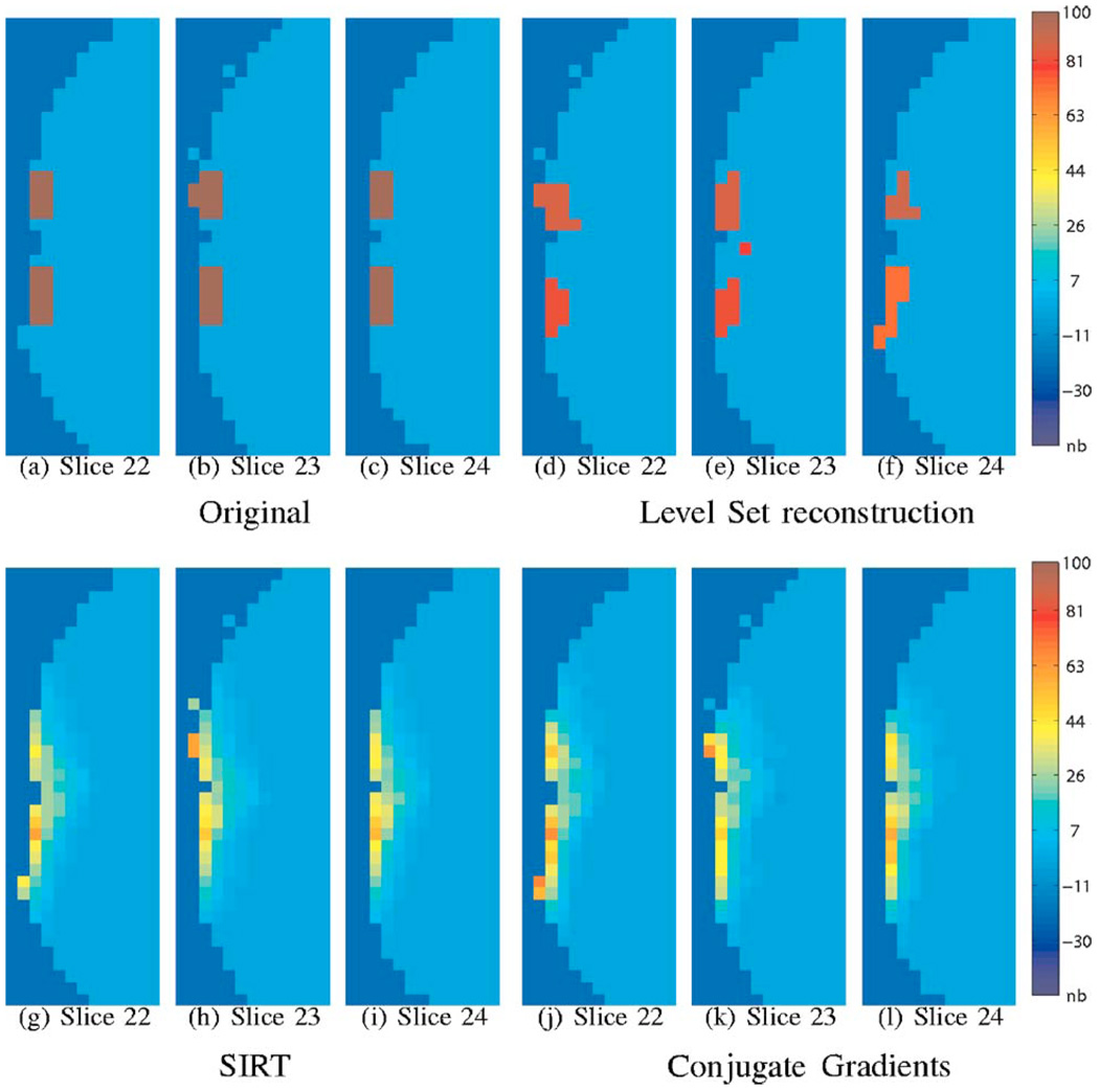
Reconstruction in the presence of noise. The range of the original signal is scaled to be in the range 0 to 100; the same scale factor is applied to the reconstructions as well. The voxel dimensions in the above figure are 4 mm³. We considered a noise process of standard deviation that is 2% of the baseline signal. We considered 50 averages of this signal and reconstructed the signal. Note that the SIRT and TCG give very smooth reconstructions. Also note that their amplitudes (from the color bar) are not in good agreement with the original. On the other hand, the level-set algorithm gave reasonable reconstructions indicating its improved resolving capability. Here we used μ = 2e−3, λ = 0.3, ζ =0.8. Note that the optimal parameter set depends on the noise level and hence is different from the noise-free case considered in Fig. 3.

The optimal parameters (number of iterations in TCG and SIRT and the variables λ, μ, and ζ in the new algorithm) are determined by comparing the reconstructions to the original, for a typical perturbation. This perturbation is different from the ones considered in the subsequent experiments, which are reported in this paper. This optimal parameter set, so derived, was then used for all experiments at this noise level. Since the parameters depend on the noise level, the optimal parameter set has to be determined for each noise level. Because this set is a function of the noise levels, the experiment had to be repeated for different noise levels (or number of averages).

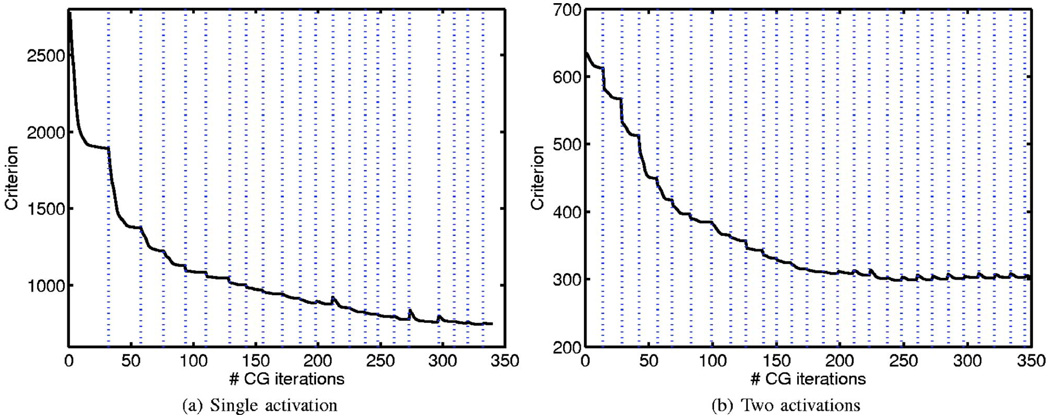
The algorithm is implemented in MATLAB, with a C implementation of the support update. The decay of the criterion in Eq. (10) as a function of the number of CG iterations in the cases of single-blob and two-blob perturbations (Fig. 3 and Fig. 4) are shown in Fig. 5. It is seen that the criterion decreases rapidly after every support update. The level-set algorithm on the average took ~1 min to converge in comparison to ~10 s for the TCG on a Pentium 4, 3.2 GHz computer.

Fig. 5.

Decay of the criterion (10) as a function of the number of CG iterations. The dotted lines mark the locations of the level-set update, where the support of the activations are changed. Each support update will add or delete new voxels to the current estimate of the support. The newly added voxels are initialized by zeros to start the CG iteration. This results in a slight increase in the value of the criterion [mainly due to a high value of the third term in Eq. (10)] after some of the support updates (at the steps where new voxels are added). Note that in these steps, the criterion decays to a value smaller than the one before the support update in a few iterations. Both the CG and the level-set iterations are terminated when the relative decrease in the criterion falls below a specified threshold.

3.1.1 Qualitative comparisons

In this section, we perform qualitative comparisons of the three algorithms: SIRT, TCG, and level set. First, we compare them in the absence of noise. A few slices of the original and the reconstructed activations are overlaid on the mask of the brain (gray-matter and white-matter regions) in Fig. 3. Note that the SIRT and CG reconstructions are distributed over a much larger region of the mask. There are also some regions on these estimates where the reconstructions are oscillatory (the white arrows in the figure show regions of negative amplitudes). The noisy-looking reconstructions of the CG could be due to the oscillatory nature of the singular vectors of the system matrix A. These oscillatory reconstructions were also reported in Ref. 16. On the other hand, the new approach gives reconstructions that are similar to the original signal.

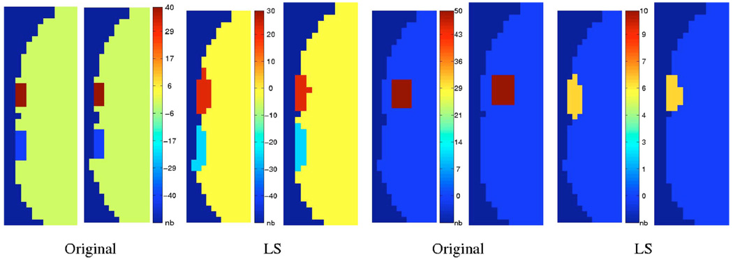
To understand the flexibility and limitations of the algorithm, we study the performance of the algorithm for two different activations in Fig. 6. In the first case, we consider two blobs with different amplitudes. It is seen that the level-set algorithm provides a reasonably good recovery of the amplitudes and the shape of the reconstructions. We then considered a single activation that is deeper in the brain. In this case, the reconstructions are biased to the cortical surface as expected. This is due to the exponential drop in sensitivity of the optical technique with depth. With standard reconstruction schemes, this bias is predominant and often leads to artifacts as seen in Fig. 9.

Fig. 6.

Reconstruction for various test activation patterns. Two adjacent slices of each data set are displayed. We consider an activation pattern with two blobs that have different amplitudes on the left. It is seen that the level-set reconstruction scheme give a reasonably good reconstruction of the activations. On the right, we test the reconstructions for a deeper activation. It is seen that the level-set reconstructions are biased to the surface of the cortex. Also note that the amplitude of the reconstructions are much lower than the original value. This is because light bundles decay exponentially with depth. Here, we used the same noise level and same parameters as in Fig. 4.

Fig. 9.

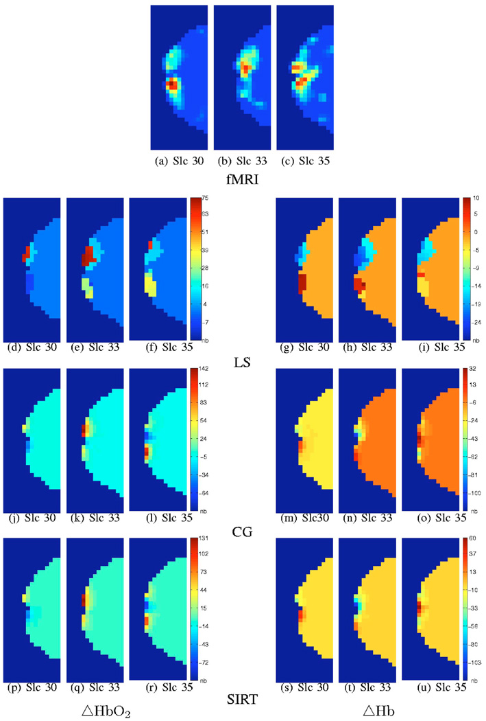
Reconstruction of perturbation in oxyhemoglobin (ΔHbO₂) and deoxyhemoglobin (ΔHb) concentrations (in nanomoles/liter) in comparison with the fMRI maps. Because many averages were used to suppress the noise, we used the same parameter set as in Fig. 3. The reconstructions are constrained to the brain (gray matter and white matter). Three slices overlaid on the mask of the brain are displayed. As expected, the NIRSI reconstructions are biased to the cortical surface due to the exponential decay of sensitivity with depth. However, in comparision to CG and SIRT, the level-set reconstructions more closely resemble the fMRI activation maps.

In Fig. 4, we study the case where there are two activated regions in the presence of noise. Note that the SIRT and TCG algorithms give a uniformly smooth reconstruction; these algorithms are not capable of resolving the two activations. On the other hand, the new algorithm results in two distinct activations, although the shapes are distorted. This clearly indicates that the new approach can resolve adjacent structures better.

3.1.2 Quantitative comparisons

In this section, we compare the different algorithms by comparing the estimates with the original signal f_orig. Here, we considered the case with only one activation. We use different metrics for comparison:

1. Mean squared error (MSE)

The normalized mean squared error in estimation is given by

$$\text{MSE}=\frac{{\displaystyle {\int }_{{ℝ}^3}|f_{\text{orig}}(\mathbf{x})-f_{\text{est}}(\mathbf{x}){|}^2\mathrm{d}\mathbf{x}}}{{\displaystyle {\int }_{{ℝ}^3}|f_{\text{orig}}(\mathbf{x}){|}^2\mathrm{d}\mathbf{x}}}.$$ (23)

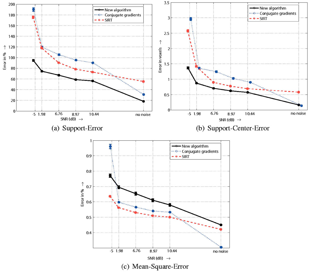
While this error term is widely used and is simple, its value can be misleading in our setting. The level-set algorithm produces piecewise smooth reconstructions as compared to smooth reconstructions with SIRT and CG. Because the optical light bundles are smooth and few in number, it is not possible to precisely localize the functional activations. The MSE would indicate larger errors for the level-set method, even when the piecewise smooth reconstructions are only slightly off. On the other hand, this metric gives small values while comparing smooth functions, even when the locations are wrong.

2. Support error (SE)

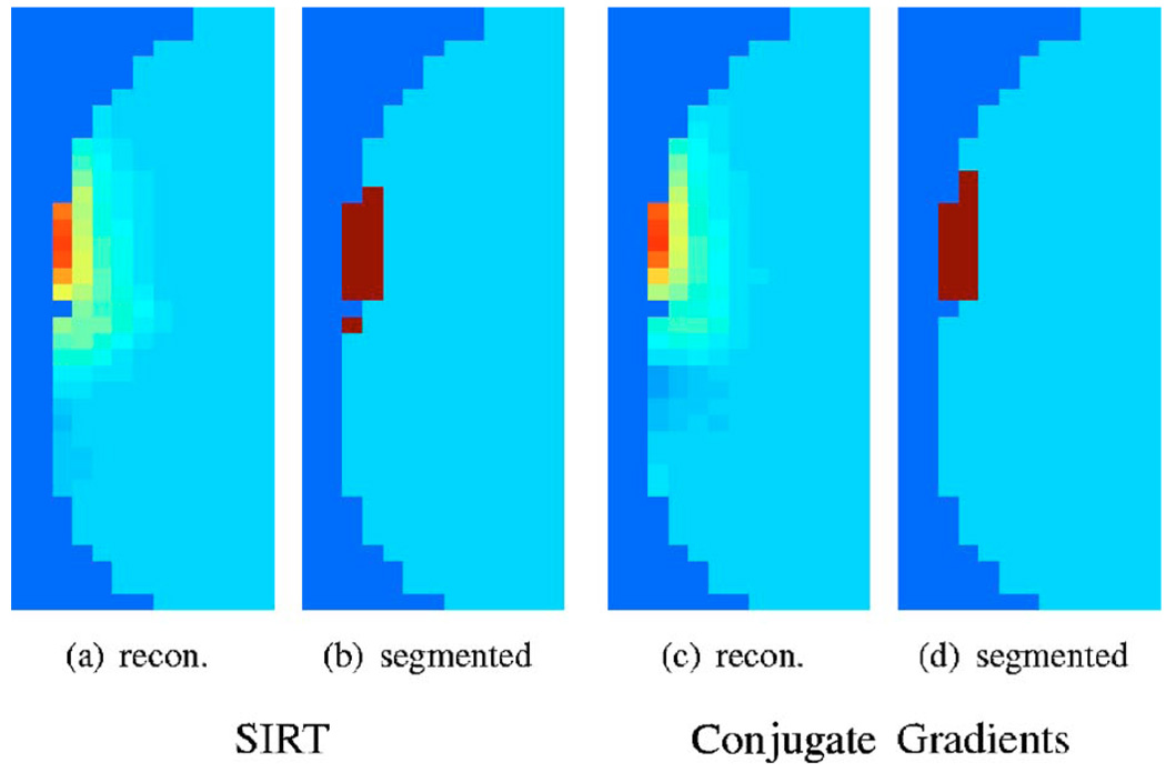
We use the standard MATLAB (Math-works, Natick, New Jersey) implementation of the k-means algorithm to classify the reconstructions into two regions (activated and background). Examples of the segmentations of CG and SIRT reconstructions are shown in Fig. 7. We then compare the support of the estimated activations to the original support using the metric

$$\text{SE}=\frac{{\displaystyle {\int }_{{ℝ}^3}|{\mathit{\chi }}_{{\mathrm{\Omega }}_{\text{orig}}}(\mathrm{x})-{\mathit{\chi }}_{{\mathrm{\Omega }}_{\text{est}}}(\mathbf{x}){|}^2\mathrm{d}\mathbf{x}}}{{\displaystyle {\int }_{{ℝ}^3}|{\mathit{\chi }}_{{\mathrm{\Omega }}_{\text{orig}}}(\mathbf{x}){|}^2\mathrm{d}\mathbf{x}}},$$ (24)

where the characteristic function of a region Ω is defined as

$${\mathit{\chi }}_{\mathrm{\Omega }}(\mathbf{x})=\{\begin{array}{cc}1,\hfill & \text{if}\mathbf{x}\in \mathbf{\Omega },\hfill \\ 0,\hfill & \text{otherwise}.\hfill \end{array}$$ (25)

Fig. 7.

Examples of segmentations of a slice of the reconstructions using k-means algorithm. The error between the original support and the segmentation is used as a criterion for comparison. See Sec. 3.1.2 for details.

Note that the above metric counts the misclassified voxels in the reconstruction and hence ignores any amplitude changes. This metric can be argued to make better sense for the comparison of reconstructions of functional activations.

3. Support centroid error (SCE)

We choose the distance between the centroids of the original activation and that of the detected activation as the error measure. This approach uses the classification from the earlier metric.

Using these error measures, we quantitatively compare the performance of the algorithms (level-set, CG, and SIRT) as a function of the number of averages for the single activation case (Fig. 3). Note that the SNR is proportional to the square root of the number of averages. The results are displayed in Fig. 8. Note that the new algorithm fares better under both SE and SCE, in clear agreement to the visual comparisons. However, the MSE indicates a higher error in comparison to the others. As we have explained before, this is due to the inherent weakness of MSE to compare piecewise constant functions. Note that the errors of any of the algorithms does not decay to zero even when there is no noise, indicating the insufficiency of the data (ill-posed nature of the problem).

Fig. 8.

Quantitative comparison of the performance of the algorithms to noise. We plot the reconstruction error, evaluated using different metrics, as a function of the SNR of the measurements. Note that the level-set algorithm fares significantly better than the other under the SE and SCE criteria, in clear agreement with the visual comparisons. The MSE criterion indicates worse results. As discussed below, this is mainly due to the limitation of the MSE in comparing two piecewise constant functions.

3.2 Experimental Results

We now study the performance of the algorithm to experimental data. The optical probe was designed with 16 pairs of 400-mm-diameter core plastic-clad multimode silica source fibers and 4 detector fiber bundles. The topology of the probe is shown in Fig. 1. A MRI visible marker is attached adjacent to each of the 16 optical source fibers and 4 detector fiber bundles so that accurate source and detector positions could be estimated from MR images. Experimental fMRI and NIRSI data were obtained from a normal subject, who was scanned using a Siemens Allegra 3T system. The study was approved by the University of Illinois at Urbana-Champaign Institutional Review Board. Written informed consent was obtained from the volunteer before the study began.

The optical signals were recorded using a near-infrared spectrometer (Imagent, ISS, Champaign, Illinois). Data acquisition was synchronized with the fMRI measurements using the transistor-transistor logic (TTL)-trigger signal from the MR scanner, which also triggered the beginning of the visual stimulation paradigm. The optical sources were laser diodes (690 and 830 nm) that are amplitude modulated at 150 MHz and time-multiplexed. Light reaching the detectors was amplified by photomultiplier tubes and converted into ac, dc, and phase signals for each of the source-detector combinations, or channels, at each wavelength.

A pair of nonmagnetic goggles (Resonance Technology, Inc., North Ridge, California) with liquid crystal display screens were placed in front of the subjects’ eyes inside the birdcage head coil. The visual stimulation paradigm consisted of five blocks each with 28.8-s fixation followed by 19.2 s of a black-and-white checkerboard pattern flashing on for 50 ms and off for 1.95 s.

Automatic estimation of source and detector positions from the MR images, incorporating deformation of the optical probe, is performed using custom-developed image processing algorithms written in MATLAB. The optical data is averaged over 80 activation-relaxation trials to produce the estimate of the signal difference between the active and baseline conditions.¹⁶ The level-set reconstructions of the perturbation in absorption coefficients are performed at the two wave-lengths. The perturbation in the oxy- and the deoxyhemoglobin concentrations are estimated using the Lambert-Beer law.

The estimated perturbation maps, overlaid on the brain surface, are shown in Fig. 9. One would expect a systematic increase and decrease in the oxy- and deoxyhemoglobin concentrations, respectively, at the locations corresponding to the fMRI activations. It is seen from the reconstructions that this is roughly the trend in the NIRSI reconstructions. However, unlike the fMRI image, both CG and SIRT reconstructions indicate activations in a shallow region of the brain without separation between left and right sides of the visual cortex. On the contrary, the level-set images show two separate activated regions on the left and right sides of the brain, which are deeper and similar to the fMRI images. All optical images show stronger activation in the left hemisphere because in this location the activation region (as revealed by fMRI) is slightly closer to the surface of the head.

4 Conclusions

We have proposed a new reconstruction algorithm to estimate the functional activations for diffuse optical imaging of functional activations in the human brain. Our approch relies on penalty terms that agree with the physiological properties of the activated regions in the brain to make the problem well-posed. Hence, it produced reconstructions with better spatial resolution and fewer artifacts, as compared to the existing techniques. The main downside of the algorithm is the computational complexity; the new approach is about 5 to 10 times more expensive than the standard algorithms. However, as computers are getting more powerful, this issue becomes less of a concern. We compared the algorithm with two standard reconstruction techniques: SIRT and TCG on both simulated and experimental data; the results clearly demonstrate the improvement in resolution and robustness over the existing algorithms.

Appendix A—Derivation of the Optimal f Given Ω

To derive the optimal f, we need to solve the problem

$$f^{*}=\underset{f}{\text{arg min}}\frac{(\Vert \mathbf{y}-{\mathbf{\Lambda }}_{\mathrm{\Omega }}f{\Vert }^2+\mu {\displaystyle {\int }_{\mathrm{\Omega }}|f{|}^2\mathrm{d}\mathbf{x}+\mathrm{\lambda }}{\displaystyle {\int }_{\mathrm{\Omega }}|\mathbf{\nabla }f{|}^2\mathrm{d}\mathbf{x})}.}{c(f)}$$ (26)

Perturbing f to f + δ, the corresponding perturbation in the cost function is

$$\begin{array}{cc}\mathbf{\Delta }𝒞=\hfill & 𝒞(f+\delta )-𝒞(f)\approx 2\langle {\mathbf{\Lambda }}_{\mathrm{\Omega }}\delta ,(\mathbf{y}-{\mathbf{\Lambda }}_{\mathrm{\Omega }}f)\rangle \hfill \\ \hfill & +2\mu {\displaystyle {\int }_{\mathrm{\Omega }}f(\mathbf{x})\delta (\mathbf{x})\mathrm{d}\mathbf{x}+2\mathrm{\lambda }}{\displaystyle {\int }_{\mathrm{\Omega }}[\mathbf{\nabla }f(\mathbf{x})·\mathbf{\nabla }\delta (\mathbf{x})]\mathrm{d}\mathbf{x}.}\hfill \end{array}$$ (27)

Using Green’s first identity, we rewrite the last term as

$$\begin{array}{cc}{\displaystyle {\int }_{\mathrm{\Omega }}[\mathbf{\nabla }f(\mathbf{x})·\mathbf{\nabla }\delta (\mathbf{x})]\mathrm{d}\mathbf{x}=}\hfill & -{\displaystyle {\int }_{\mathrm{\Omega }}\delta (\mathbf{x}){\mathbf{\nabla }}^{2}f(\mathbf{x})\mathrm{d}\mathbf{x}}\hfill \\ \hfill & +{\displaystyle {\int }_{\partial \mathrm{\Omega }}\delta (\mathbf{x})[\mathbf{\nabla }f(\mathbf{x})·d𝒩],}\hfill \end{array}$$ (28)

where 𝒩 is the unit outward normal of the surface dΩ. Combining the above result with Eq. (27), we obtain

$$\begin{array}{cc}\mathbf{\Delta }𝒞=\hfill & 2{\displaystyle {\int }_{\mathrm{\Omega }}\delta (\mathbf{x})[{\mathbf{\Lambda }}_{\mathrm{\Omega }}^H(\mathbf{y}-{\mathbf{\Lambda }}_{\mathrm{\Omega }}f)+\mu f-\mathrm{\lambda }{\mathbf{\nabla }}^{2}f]\mathrm{d}\mathbf{x}}\hfill \\ \hfill & +{\displaystyle {\int }_{d\mathrm{\Omega }}\delta (\mathbf{\nabla }f·\mathrm{d}𝒩).}\hfill \end{array}$$ (29)

At a local minimum, Δ𝒞 should be zero for any δ. This is true if and only if the conditions below hold

$${\mathbf{\Lambda }}_{\mathrm{\Omega }}^H(\mathbf{y}-{\mathbf{\Lambda }}_{\mathrm{\Omega }}f)+\mu f-\mathrm{\lambda }{\mathbf{\nabla }}^{2}f=0\text{on}\mathbf{\Omega },$$ (30)

$$\mathbf{\nabla }f·𝒩=0\text{on}\mathrm{d}\mathbf{\Omega },$$ (31)

where 𝒩 denotes the unit normal of the surface.

Appendix B—Derivation of the Optimal Velocity Given f

In this appendix, we derive the optimal boundary velocity. The standard procedure involves the construction of a family of deformed shapes Ω_t:Ω₀ = Ω, parametrized by an arbitrary parameter t such that 0 ≤ t ε. Usually, the deformations are obtained by evolving the boundary of Ω by tv(x), where v is an arbitrary velocity.

Let us assume the cost function defined by the region integral J(Ω) = ∫_Ωg(x) dx, where g:ℝ²→ℝ. From the results in continuum mechanics, the shape derivative of J under the above transformation is given by Ref. 44

$$\frac{\partial J({\mathbf{\Omega }}_t)}{\partial t}=\underset{t\to 0}{\text{lim}}\frac{J_{{\mathrm{\Omega }}_t}-J_{\mathrm{\Omega }}}{t}={\displaystyle {\int }_{\partial \mathrm{\Omega }}g\mathbf{v}\mathrm{·}\mathrm{d}𝒩}.$$ (32)

Our goal is to find the optimal velocity v(x), such that deforming Ω with v would maximally decrease J (minimize the shape derivative). Note that the shape derivative involves the integral of the inner product between g(x)d𝒩 and v(x). Using the Cauchy-Schwartz inequality, one can obtain the optimal velocity as −R_e[g(x)]𝒩.

The last three terms in Eq. (10) are region integrals. Hence, the shape derivative of these three terms is given by

$$\frac{\partial ({𝒞}_2+{𝒞}_3+{𝒞}_4)}{\partial t}={\displaystyle {\int }_{\partial \mathrm{\Omega }}(\mu |f{|}^2+\mathrm{\lambda }|\mathbf{\nabla }f{|}^2+\zeta )\mathbf{v}·\mathrm{d}𝒩.}$$ (33)

Using the chain rule of differentiation on the first term of Eq. (10) and invoking Eq. (32), we obtain

$$\frac{\partial {𝒞}_1({\mathrm{\Omega }}_t)}{\mathrm{d}t}=2\underset{{\mathbf{e}}^H}{\underbrace{{\left({\displaystyle {\int }_{\mathrm{\Omega }}\mathit{\kappa }f\mathrm{d}\mathbf{x}-\mathbf{y}}\right)}^H}}{\displaystyle {\int }_{\mathbf{d}\mathbf{\Omega }}(\mathit{\kappa }f\mathbf{v}·\mathbf{d}𝒩),}$$ (34)

$$=2{\displaystyle {\int }_{\mathrm{d}\mathrm{\Omega }}({\mathbf{e}}^H\mathit{\kappa }f)\mathbf{v}·\mathbf{d}𝒩}={\displaystyle {\int }_{\mathrm{d}\mathrm{\Omega }}2(f^{*}{\mathit{\kappa }}^H\mathbf{e})\mathbf{v}·\mathrm{d}𝒩.}$$ (35)

Combining Eq. (33) and Eq. (35) and using the argument in Eq. (32), we obtain the optimal velocity as

$${\mathbf{v}}_{\text{opt}}(\mathbf{x})=-ℝ\mathrm{e}[2f^{*}{\mathbf{\Lambda }}_{\mathrm{\Omega }}^H({\mathbf{\Lambda }}_{\mathrm{\Omega }}f-\mathbf{y})+\mu |f{|}^2+\mathrm{\lambda }|\mathbf{\nabla }f{|}^2+\zeta ]𝒩.$$ (36)

References

- 1.Yates T, Hebden JC, Gibson A, Everdell N, Arridge SR, Douek M. Optical tomography of the breast using a multi-channel time-resolved imager. Phys. Med. Biol. 2005;50:2503–2517. doi: 10.1088/0031-9155/50/11/005. [DOI] [PubMed] [Google Scholar]
- 2.Arridge SR. Optical tomography in medical imaging. Inverse Probl. 1999;15:R41–R93. [Google Scholar]
- 3.Arridge SR, Hebden JC. Optical imaging in medicine: II. Modelling and reconstruction. Phys. Med. Biol. 1997;42:841–853. doi: 10.1088/0031-9155/42/5/008. [DOI] [PubMed] [Google Scholar]
- 4.O’Leary MA, Boas DA, Chance B, Yodh AG. Experimental images of heterogeneous turbid media by frequency-domain diffusion-photon tomography. Opt. Lett. 1995;20:426–428. doi: 10.1364/ol.20.000426. [DOI] [PubMed] [Google Scholar]
- 5.Boas D, Franceschini MA, Dunn MA, Strangman AK. Noninvasive imaging of cerebral activation with diffuse optical tomography. In: Frostig RD, editor. In Vivo Optical Imaging of Brain Function. CRC Press; 2002. pp. 193–221. [PubMed] [Google Scholar]
- 6.Boas DA, Dale AM, Franceschini MA. Diffuse optical imaging of brain activation: Approaches to optimizing image sensitivity, resolution and accuracy. NeuroImage. 2004;No. 23:S275–S288. doi: 10.1016/j.neuroimage.2004.07.011. [DOI] [PubMed] [Google Scholar]
- 7.Wenzel R, Obrig H, Ruben J, Villringer K, Thiel A, Bernardinger J, Dirnagl U, Villringer A. Cerebral blood oxygenation changes induced by visual stimulation in humans. J. Biomed. Opt. 1996;4:399–404. doi: 10.1117/12.251465. [DOI] [PubMed] [Google Scholar]
- 8.Gratton G, Fabiani M, Corballis PM, Hood DC, Goodman-Wood MR, Hirsch J, Kim K, Friedman D, Gratton E. Fast and localized event-related optical signals (EROS) in the human occipital cortex: Comparisons with the visual evoked potential and fMRI. Neuroimage. 1997;6:168–180. doi: 10.1006/nimg.1997.0298. [DOI] [PubMed] [Google Scholar]
- 9.Fukui Y, Ajichi Y, Okada E. Monte Carlo prediction of near-infrared light propagation in realistic adult and neonatal head models. Appl. Opt. 2003;42:2881–2887. doi: 10.1364/ao.42.002881. [DOI] [PubMed] [Google Scholar]
- 10.Zhu W, Wang Y, Deng Y, Yao Y, Barbour RL. A wavelet based multiresolution regularized least squares reconstruction approach for optical tomography. IEEE Trans. Med. Imaging. 1997;16:210–217. doi: 10.1109/42.563666. [DOI] [PubMed] [Google Scholar]
- 11.Hielscher AH, Klose AD, Hanson KM. Gradient-based iterative image reconstruction scheme for time-resolved optical tomography. IEEE Trans. Med. Imaging. 1999;18:262–271. doi: 10.1109/42.764902. [DOI] [PubMed] [Google Scholar]
- 12.Matson CL, Clark N, McMackin L, Fender JS. Three dimensional tumor localization in thick tissue with the use of photon density waves. Appl. Opt. 1997;36:214–220. doi: 10.1364/ao.36.000214. [DOI] [PubMed] [Google Scholar]
- 13.Matson CL, Liu H. Backpropagation in turbid media. J. Opt. Soc. Am. A. 1999;16:1999. [Google Scholar]
- 14.Bertero M, Boccacci P. Introduction to Inverse Problems in Imaging. Bristol: IOP Publishing; 1998. [Google Scholar]
- 15.Gaudette RJ, Brooks DH, DiMarzio CA, Kilmer ME, Miller EL, Gaudette T, Boas DA. A comparison study of linear reconstruction techniques for diffuse optical tomographic imaging of absorption coefficient. Phys. Med. Biol. 2000;45:1051–1070. doi: 10.1088/0031-9155/45/4/318. [DOI] [PubMed] [Google Scholar]
- 16.Zhang X, Toronov V, Webb AG. Simultaneous integrated diffuse optical tomography and functional magnetic resonance imaging of the human brain. Opt. Express. 2005;13(14):5513–5521. doi: 10.1364/opex.13.005513. [DOI] [PMC free article] [PubMed] [Google Scholar]
- 17.Pogue BW, McBride TO, Prewitt J, Osterberg UL, Paulsen KD. Spatially varying regularization improves diffuse optical tomography. Appl. Opt. 1999;38:2950–2961. doi: 10.1364/ao.38.002950. [DOI] [PubMed] [Google Scholar]
- 18.Li A, Boverman G, Zhang Y, Brooks D, Miller EL, Kilmer ME, Zhang Q, Hillman EMC, Boas DA. Optimal linear inverse solution with multiple priors in diffuse optical tomography. Appl. Opt. 2005;44:1948–1956. doi: 10.1364/ao.44.001948. [DOI] [PubMed] [Google Scholar]
- 19.Boas DA, Dale AM. Simulation study of magnetic resonance imaging guided cortically constrained diffuse optical tomography of human brain function. Appl. Opt. 2005;44:1957–1968. doi: 10.1364/ao.44.001957. [DOI] [PubMed] [Google Scholar]
- 20.Barnett AH, Culver JP, Sorensen AG, Dale A, Boas DA. Robust inference of baseline optical properties of the human head with three-dimensional segmentation from magnetic resonance imaging. Appl. Opt. 2003;42:3095–3108. doi: 10.1364/ao.42.003095. [DOI] [PubMed] [Google Scholar]
- 21.Barbour RL, Graber HL, Pei Y, Zhong S, Schmitz CH. Optical tomographic imaging of dynamic features of densescattering media. J. Opt. Soc. Am. A. 2001;18(12):3018–3036. doi: 10.1364/josaa.18.003018. [DOI] [PubMed] [Google Scholar]
- 22.Bresler Y, Feng P. Spectrum-blind minimum-rate sampling and reconstruction of 2-D multiband signals. Proc. 3rd IEEE Int. Conf. on Image Process.; ICIP; 1996. pp. 701–704. [Google Scholar]
- 23.Donoho DL. For most large underdetermined systems of linear equations, the minimal 1-1 norm near-solution approximates the sparsest near-solution. 2005 preprint. [Google Scholar]
- 24.Candes E, Romberg J, Tao T. Stable signal recovery from incomplete and inaccurate measurements. 2005 preprint. [Google Scholar]
- 25.Ye JC, Bresler Y, Moulin P. A self-referencing level-set method for image reconstruction from sparse Fourier samples. Int. J. Comput. Vis. 2002;50:253–270. [Google Scholar]
- 26.Mumford D, Shah J. Optimal approximations by piecewise smooth functions and associated variational problems. Comm. Pure Apple. Math. 1989;42:577684. [Google Scholar]
- 27.Santosa F. A level-set approach for inverse problems involving obstacles. ESAIM: Control, Optimization and Calculus of Variations. 1996:1733. [Google Scholar]
- 28.Tsai A, Yezzi A, Willsky AS. Curve evolution implementation of the MumfordShah functional for image segmentation, denoising, interpolation, and magnification. IEEE Trans. Image Process. 2001;10:1169–1186. doi: 10.1109/83.935033. [DOI] [PubMed] [Google Scholar]
- 29.Osher SJ, Sethian JA. Fronts propagating with curvature dependent speed: Algorithms based on Hamilton-Jacobi formulation. J. Comp. Physiol. 1988;79:1249. [Google Scholar]
- 30.Sapiro G. Geometric Partial Differential Equations and Image Analysis. Cambridge, U.K.: Cambridge Univ. Press; 2001. [Google Scholar]
- 31.Fishkin JB, Gratton E. Propagation of photon density waves in strongly scattering media containing an absorbing semi-infinite plane bounded by a straight edge. J. Opt. Soc. Am. A. 1993;10:127–140. doi: 10.1364/josaa.10.000127. [DOI] [PubMed] [Google Scholar]
- 32.Boas DA, Culver JP, Stott JJ, Dunn AK. Three dimensional Monte-Carlo code for photon migration through complex heterogeneous media including adult human head. Opt. Express. 2002;10:159–170. doi: 10.1364/oe.10.000159. [DOI] [PubMed] [Google Scholar]
- 33.Gratton E, Toronov V, Wolf U, Webb A. Measurement of brain activity by near-infrared light. J. Biomed. Opt. 2005;16 doi: 10.1117/1.1854673. 011008. [DOI] [PubMed] [Google Scholar]
- 34.Venkataramani R, Bresler Y. Further results on spectrum blind sampling of 2D signals. Proc. IEEE Int. Conf. Image Process.; ICIP; 1998. pp. 756–752. [Google Scholar]
- 35.Feng H, Karl WC, Castanon DA. A curve evolution approach to object-based tomographic reconstruction. IEEE Trans. Image Process. 2003;12(1):44–57. doi: 10.1109/TIP.2002.806253. [DOI] [PubMed] [Google Scholar]
- 36.Shi Y, Karl WC, Castanon DA. Dynamic tomography using curve evolution with spatial-temporal regularization. IEEE Int. Conf. Image Process.; Rochester. 2002. [Google Scholar]
- 37.Shi Y. Ph.D. Thesis. Boston University: 2005. Object-Based Dynamic Imaging with Level-Set Methods. [Google Scholar]
- 38.Yu DF, Fessler J. Edge-preserving tomographic reconstruction with nonlocal regularization. IEEE Trans. Med. Imaging. 2002;21(2):159–173. doi: 10.1109/42.993134. [DOI] [PubMed] [Google Scholar]
- 39.Kilmer ME, Miller EL, Barbaro A, Boas DA. Three dimensional shape-based imaging of absorption perturbation for diffuse optical tomography. Appl. Opt. 2003;42(16):3129–3144. doi: 10.1364/ao.42.003129. [DOI] [PubMed] [Google Scholar]
- 40.Kass M, Witkin A, Terzopoulos D. Snakes: Active contour models. Int. J. Comput. Vis. 1988;1:321–332. [Google Scholar]
- 41.Jacob M, Blu T, Unser M. Efficient energies and algorithms for parametric snakes. IEEE Trans. Image Process. 2004;13:1231–1244. doi: 10.1109/tip.2004.832919. [DOI] [PubMed] [Google Scholar]
- 42.Gomes J, Faugeras O. Reconciling distance functions and level sets. Inria Research Report. 1999:3666. [Google Scholar]
- 43.Malladi R, Sethian A, Vemuri BC. Shape modeling with front propagation. A level set approach. IEEE Trans. Pattern Anal. Mach. Intell. 1995;17:158–175. [Google Scholar]
- 44.Sokolowski J, Zolesio J. Introduction to Shape Optimization: Shape Sensitivity Analysis. New York: Springer-Verlag; 1991. [Google Scholar]