Genome analysis with inter-nucleotide distances

Abstract

Motivation: DNA sequences can be represented by sequences of four symbols, but it is often useful to convert the symbols into real or complex numbers for further analysis. Several mapping schemes have been used in the past, but they seem unrelated to any intrinsic characteristic of DNA. The objective of this work was to find a mapping scheme directly related to DNA characteristics and that would be useful in discriminating between different species. Mathematical models to explore DNA correlation structures may contribute to a better knowledge of the DNA and to find a concise DNA description.

Results: We developed a methodology to process DNA sequences based on inter-nucleotide distances. Our main contribution is a method to obtain genomic signatures for complete genomes, based on the inter-nucleotide distances, that are able to discriminate between different species. Using these signatures and hierarchical clustering, it is possible to build phylogenetic trees. Phylogenetic trees lead to genome differentiation and allow the inference of phylogenetic relations. The phylogenetic trees generated in this work display related species close to each other, suggesting that the inter-nucleotide distances are able to capture essential information about the genomes. To create the genomic signature, we construct a vector which describes the inter-nucleotide distance distribution of a complete genome and compare it with the reference distance distribution, which is the distribution of a sequence where the nucleotides are placed randomly and independently. It is the residual or relative error between the data and the reference distribution that is used to compare the DNA sequences of different organisms.

Contact: vera@ua.pt

1 INTRODUCTION

DNA sequences have been converted to numerical signals using different mappings. A commonly used mapping is to consider binary sequences that describe the position of each symbol (Voss, 1992). The binary representation is certainly one of the earliest and one of most popular mappings of DNA. However, several other different mappings have been proposed (Akhtar et al., 2007; Anastassiou, 2001; Brodzik and Peters, 2005; Buldyrev et al., 1995; Cristea, 2003; Jeffrey, 1990; Liao et al., 2005; Nair and Mahalakshmi, 2005; Ning et al., 2003; Randic, 2008; Silverman and Linsker, 1986; Zhang and Zhang, 1994).

Some of the mappings used in DNA processing do not have a simple numerical interpretation and others do not have biological motivation. Also, some of the representations are not reversible and do not take into account the sequence structure. Currently, there is no ideal mapping to analyze every type of correlation in DNA sequences.

The inter-nucleotide distances introduced by Nair and Mahalakshmi (2005) provides a new DNA numerical methodology profile and a new mapping to explore the correlation structure of DNA. This representation converts any DNA sequence into a unique numerical sequence with the same length, where each number represents the distance of a symbol to the next occurrence of the same symbol. The global inter-nucleotide distance representation is reversible, but does not explore the individual behavior of each nucleotide.

We explore the inter-nucleotide representation introduced by Nair and Mahalakshmi (2005) and develop new methodologies to analyze this representation and extract some interesting features of the DNA correlation structure. Nair and Mahalakshmi (2005) applied Fourier analysis to the distance sequence and showed that this mapping has a discriminatory capability for highlighting the promoter region of gene sequences. However, Akhtar and Epps (2008) found that it has poor exon prediction accuracy.

In our approach, we introduced four sequences, one for each nucleotide, to represent the inter-nucleotide distances. This methodology allows to perform comparative analysis between the behavior of the four nucleotides and of the global sequence. We studied the five inter-nucleotide distance distributions and we present one residual analysis to characterize organisms and to do multiple organism comparisons.

Phylogenetic trees reproduce the evolutionary tree that represents the historical relationships between the species. Recent phylogenetic tree algorithms use nucleotide sequences. Typically, these trees are constructed with multiple sequence alignment (Hodge and Cope, 2000), which is a computationally demanding task. We propose an algorithm based on the inter-nucleotide distance behavior that is capable of efficiently building phylogenetic trees.

2 METHODS

Consider the alphabet 𝒜={A, C, G, T} and let s=(s_k)_{k∈{1,…,N}} be a symbolic sequence defined in 𝒜. Consider a numerical sequence, d^x, that represents the inter-nucleotide distances to the symbol x∈𝒜. We show below, as an example, the four inter-nucleotide distance sequences for a short DNA fragment AAACCCGTGTCAGTT:

considering that the symbolic sequence is cyclic.

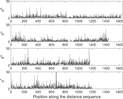
It is possible, for small sequences, to visualize the four inter-nucleotide distance sequences, as exemplified in Figure 1 for gene gi|33286443|ref|NM_032427.1 from H.sapiens.

Fig. 1.

Inter-nucleotide distances for the gi|33286443|ref|NM_032427.1 gene of Homo sapiens.

Another distance sequence, originally introduced by Nair and Mahalakshmi (2005), is the global inter-nucleotide distance sequence, d. This global distance sequence is exemplified below for the same short DNA segment used previously,

which is slightly different from the non-cyclic approach used by Nair and Mahalakshmi (2005).

The length (N) of the global distance sequence, d, is equal to the sum of the lengths of the four inter-nucleotide distance sequences (N^A, N^C, N^G and N^T). Thus,

If the positions of the first occurrence of each nucleotide are known, k₀^A, k₀^C, k₀^G and k₀^T (s_k0^x=x and s_l≠x for 0<l<k₀^x), then the positions of all the nucleotides in the complete sequence may be determined from the inter-nucleotide distance sequences,

Naturally, we have: k_j^x−k_j−1^x=d_j^x and N=∑_i∈N^xd_i^x, x∈𝒜.

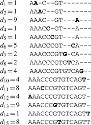
In order to illustrate the reversibility of the mapping, we show how to reconstruct the DNA sequence used in the example above from the initial positions of the symbols and the global distance sequence. We start by assigning the first symbols to their positions in the sequence,

Then considering each distance in the sequence we reconstruct iteratively the symbol sequence

There is some redundancy in the four inter-nucleotide distance sequences and three of them would be sufficient to determine the complete nucleotide sequence.

2.1 Distribution of the distance sequences

In order to calculate some statistical properties of various genomes, we will study the characteristics of the inter-nucleotide distance distribution.

Consider p^A, p^C, p^G and p^T as the occurrence probabilities of nucleotides A, C, G and T, respectively. If the nucleotide sequences were generated by an independent and identically distributed (i.i.d.) random process, then each of the inter-nucleotide distance sequences, d^x, would follow a geometric distribution. In fact, the probability distribution of the inter-nucleotide distances of the symbol x is

its distribution function is

the expected value is 1/p^x and the variance is (1 − p^x)/(p^x)². To estimate the nucleotide occurrence probability, p^x, we use relative frequencies, N^x/N, computed from the original nucleotide sequence. The term reference distribution, applied to a DNA sequence, describes the distribution that the inter-nucleotide distances for that sequence would follow, if its nucleotides were randomly determined, with probabilities equal to the relative frequencies, independently of each other.

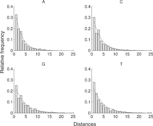
Figure 2 shows the measured and the reference distributions of the inter-nucleotide distance sequences for gi|33286443|ref|NM_032427.1 gene of H.sapiens. Although the nucleotide distance distribution from DNA shows a power law behavior, it differs from the reference distribution. This power law behavior is expected, since the reference distribution was established under the assumption of a i.i.d. random process (with constant nucleotide relative frequencies estimated from the DNA sequence).

Fig. 2.

Distribution of the 4 nt distance sequences for gene gi|33286443|ref|NM_032427.1 of H.sapiens. The histogram is from the observed distances and the solid line shows the reference distribution with parameters estimated from the data.

To compare the distribution of the inter-nucleotide distance sequences with the reference distribution several measures may be used. Some examples are the Kolmogorov–Smirnov distance, Kullback–Leibler distance and the correlation coefficient. In this work, we use the Kolmogorov–Smirnov distance to assess how significantly different the distribution of the measured distance sequence and the reference distribution are. The comparison between the distribution obtained from the data and the reference distribution may be carried out for the nucleotide distance sequences and also for the global distance sequence.

As mentioned above, the reference distance distribution for each nucleotide is geometric, assuming that the DNA sequence was generated by an independent random process with constant parameters, and the corresponding global distance sequence distribution is given by

2.2 DNA sequences

In this study, we used the complete DNA sequences of 28 species: 26 were obtained from the National Center for Biotechnology Information (NCBI; ftp://ftp.ncbi.nih.gov/genomes/); Populus trichocarpa (California poplar) obtained from the Joint Genome Institute (http://genome.jgi-psf.org/) and Xenopus tropicalis (Western clawed frog) from Xenbase (http://www.xenbase.org/).

The species used in this work are listed in Table 1.

Table 1.

List of DNA builds used for each species

Species	Reference
Homo sapiens (human)	Build 36.3
Pan troglodytes (chimpanzee)	Build 2.1
Macaca mulatta (Rhesus macaque)	Build 1.1
Mus musculus (mouse)	Build 37.1
Rattus norvegicus (brown rat)	Build 4.1
Equus caballus (horse)	Build 2.1
Cannis familiaris (dog)	Build 2.1
Bos taurus (cow)	Build 4.1
Ornithorhynchus anatinus (platypus)	Build 1.1
Gallus gallus (chicken)	Build 2.1
Xenopus tropicalis (Western clawed frog)	Build 4.1
Danio rerio (zebrafish)	Build 3.1
Apis mellifera (honey bee)	Build 4.1
Caenorhabditis elegans (nematode)	NC003279
Vitis vinifera (grape vine)	Build 1.1
Populus trichocarpa (California poplar)	Build 1.0
Arabidopsis thaliana (thale cress)	AGI 7.2
Saccharomyces cerevisiae str.S228C (budding yeast)	SGD 1
Schizosaccharomyces pombe (fission yeast)	Build 1.1
Dictyostelium discoideum str.AX4 (amoeba)	Build 2.1
Plasmodium falciparum 3D7 (protozoon)	Build 2.1
Escherichia coli str.K12 substr.MG1655 (bacterium)	NC000913
Bacillus subtilis str.168 (bacterium)	NC000964
Chlamydia trachomatis str.D/UW-3/CX (bacterium)	NC000117
Mycoplasma genitalium str.G37 (bacterium)	NC000908
Streptococcus mutans str.UA159 (bacterium)	NC004350
Streptococcus pneumoniae str.ATCC 700669 (bacterium)	NC011900
Aeropyrum pernix str.K1 (archaeota)	NC000854

2.3 Experimental procedure

The histograms of the distance sequences were computed for each nucleotide and also for the global sequence. For large genomes, the sequences were divided into blocks of 500 000 symbols and the continuity from block to block was guaranteed. For eukaryote genomes, the chromosomes were processed separately and the resulting distance histograms were stored separately. All the symbols in the sequence that did not correspond to one of the four nucleotides were removed from the sequences before further processing.

We setup to investigate how similar (or different) are the distance distributions and the reference distributions of:

• the four nucleotides of H.sapiens;

• the chromosomes of H.sapiens;

• various species.

In order to facilitate the visual comparison of the various distance distributions with the theoretical one, we used the relative error, as given by

(1)

where f_o(k) is the observed relative frequency of the distance k, and f(k) is the relative frequency of the reference distribution.

It is known that coding regions usually have different characteristics when compared with the complete genome. To explore these differences, we carried out an experiment to compare the behavior of the global distance distributions of the complete genome and coding regions of H.sapiens. The distances between nucleotides within each gene were considered as separate sequences and the distance distribution was computed from all the genes. The data for the human coding regions was obtained from the RNA file at the NCBI ftp site.

3 RESULTS

3.1 Inter-nucleotide distances analysis

Table 2 shows the results of the Kolmogorov–Smirnov test between the distance relative frequencies distributions of all the human chromosome pairs. Only the first 100 distances were used. The results of the test show that for a significance level of 5% it is not possible to say that the distributions of the distances for the various chromosomes are different.

Table 2.

P-values from Kolmogorov–Smirnov test to compare inter-nucleotide distance relative frequencies distributions between the chromosomes of H.sapiens

	C1	C2	C3	C4	C5	C6	C7	C8	C9	C10	C11	C12	C13	C14	C15	C16	C17	C18	C19	C20	C21	C22	CX	CY
C1	1.0	1.0	1.0	1.0	1.0	1.0	1.0	1.0	1.0	1.0	1.0	1.0	1.0	1.0	1.0	0.6	1.0	1.0	0.4	1.0	0.9	1.0	1.0	0.3
C2	–	1.0	1.0	1.0	1.0	1.0	1.0	1.0	1.0	0.9	1.0	1.0	1.0	1.0	1.0	0.7	1.0	1.0	0.3	0.9	0.8	0.9	1.0	0.2
C3	–	–	1.0	1.0	1.0	1.0	0.9	1.0	1.0	0.8	1.0	1.0	1.0	1.0	1.0	0.6	1.0	1.0	0.3	0.8	0.7	0.8	1.0	0.1
C4	–	–	–	1.0	1.0	1.0	1.0	1.0	1.0	1.0	1.0	1.0	1.0	1.0	1.0	0.7	1.0	1.0	0.3	1.0	0.9	1.0	1.0	0.2
C5	–	–	–	–	1.0	1.0	1.0	1.0	1.0	1.0	1.0	1.0	1.0	1.0	1.0	0.6	1.0	1.0	0.3	1.0	0.8	1.0	1.0	0.1
C6	–	–	–	–	–	1.0	1.0	1.0	1.0	1.0	1.0	1.0	1.0	1.0	1.0	0.6	1.0	1.0	0.3	1.0	0.8	1.0	1.0	0.2
C7	–	–	–	–	–	–	1.0	1.0	1.0	1.0	1.0	1.0	1.0	1.0	1.0	0.9	1.0	1.0	0.7	1.0	1.0	1.0	1.0	0.2
C8	–	–	–	–	–	–	–	1.0	1.0	1.0	1.0	1.0	1.0	1.0	1.0	0.7	1.0	1.0	0.3	1.0	1.0	1.0	1.0	0.2
C9	–	–	–	–	–	–	–	–	1.0	1.0	1.0	1.0	1.0	1.0	1.0	0.7	1.0	1.0	0.6	1.0	0.9	0.9	1.0	0.1
C10	–	–	–	–	–	–	–	–	–	1.0	1.0	1.0	1.0	1.0	1.0	0.8	1.0	1.0	0.4	1.0	1.0	1.0	1.0	0.2
C11	–	–	–	–	–	–	–	–	–	–	1.0	1.0	1.0	1.0	1.0	0.8	1.0	1.0	0.4	1.0	0.9	0.9	1.0	0.2
C12	–	–	–	–	–	–	–	–	–	–	–	1.0	1.0	1.0	1.0	0.6	1.0	1.0	0.4	1.0	0.9	1.0	1.0	0.2
C13	–	–	–	–	–	–	–	–	–	–	–	–	1.0	1.0	1.0	0.6	1.0	1.0	0.3	1.0	0.9	1.0	1.0	0.2
C14	–	–	–	–	–	–	–	–	–	–	–	–	–	1.0	1.0	0.6	1.0	1.0	0.3	1.0	0.8	1.0	1.0	0.1
C15	–	–	–	–	–	–	–	–	–	–	–	–	–	–	1.0	0.8	1.0	1.0	0.2	1.0	0.9	1.0	1.0	0.1
C16	–	–	–	–	–	–	–	–	–	–	–	–	–	–	–	1.0	0.8	0.8	1.0	0.8	1.0	1.0	1.0	0.6
C17	–	–	–	–	–	–	–	–	–	–	–	–	–	–	–	–	1.0	1.0	0.6	1.0	1.0	1.0	1.0	0.2
C18	–	–	–	–	–	–	–	–	–	–	–	–	–	–	–	–	–	1.0	0.3	1.0	1.0	1.0	1.0	0.1
C19	–	–	–	–	–	–	–	–	–	–	–	–	–	–	–	–	–	–	1.0	0.6	0.8	0.8	0.7	0.9
C20	–	–	–	–	–	–	–	–	–	–	–	–	–	–	–	–	–	–	–	1.0	1.0	1.0	1.0	0.2
C21	–	–	–	–	–	–	–	–	–	–	–	–	–	–	–	–	–	–	–	–	1.0	1.0	1.0	0.6
C22	–	–	–	–	–	–	–	–	–	–	–	–	–	–	–	–	–	–	–	–	–	1.0	1.0	0.2
CX	–	–	–	–	–	–	–	–	–	–	–	–	–	–	–	–	–	–	–	–	–	–	1.0	0.3
CY	–	–	–	–	–	–	–	–	–	–	–	–	–	–	–	–	–	–	–	–	–	–	–	1.0

Only the first 100 distances were used.

The need for limiting the distances to the first 100 represents a compromise between two extremes. On one hand, if all or a very large number of distances are used, the distributions will be very sparse and difficult to interpret. On the other hand, if the number is too small, the vector of distances may not contain enough information about the inter-nucleotide distributions. We have found that the limitation to the first 100 distances, which was carried out in all experiments described in this article, provides an adequate compromise.

Our results confirm that the distribution of the first distances contains information about the genome of each species, and that it may be interpreted as a genetic signature. The approach is justified by the similarity between the distance relative frequencies distributions of all the chromosomes (high P-values). The same similarity was also found on the DNA of the other organisms used in this study, with some exceptions for the Gallus gallus.

We have also compared the inter-nucleotide distance relative frequencies distribution of the four nucleotides, by applying the Kolmogorov–Smirnov test to the distance relative frequencies distribution for the complete genome. The results of the comparative tests are shown in Table 3.

Table 3.

P-values from the Kolmogorov–Smirnov test to compare inter-nucleotide distance relative frequencies distributions between nucleotides in H.sapiens

	A	C	G	T
A	1	0.00032	0.00032	1
C	–	1	1	0.00058
G	–	–	1	0.00058
T	–	–	–	1

Only the first 100 distances were used.

The results in Table 3 show that the distance relative frequencies distribution of the nucleotide A is identical to that of the nucleotide T, and the distance relative frequencies distribution of C is identical to that of G, but the distributions for A (or T) and C (or G) are significantly different. Notice that the DNA complementary sequence was not used in the computation of the inter-nucleotide distance distribution. These identical distance distributions for the nucleotides A/T and C/G are present in all the human chromosomes and also on the genome of all the other species used in this work.

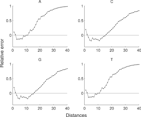
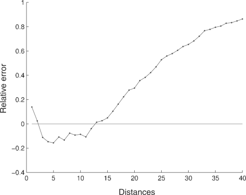
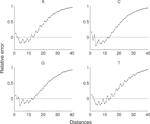
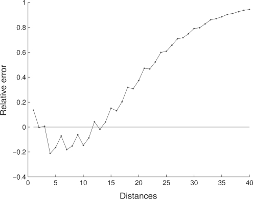
We may use the relative error, as defined in (1), to compare the distance distributions, both for inter-nucleotide and global sequences, with the reference distributions. Figure 3 shows the relative error for the inter-nucleotide distance in H.sapiens and Figure 4 shows the relative error for the global distance.

Fig. 3.

Relative error for the nucleotide distance distribution in the complete genome of H.sapiens. For convenience, only the first 40 distances are displayed.

Fig. 4.

Relative error for the global distance distribution in the complete genome of H.sapiens. For convenience, only the first 40 distances are displayed.

For the human genome, the first two distances have a higher frequency than the corresponding random sequences, and the following 10 distances have lower frequencies. For distances higher than 12 the relative error is always positive (this behavior is similar in all chromosomes). The higher frequencies of the first two distances of the human genome highlight constitutive repeat elements [see Doggett (2001) for an overview of repeating structures in the human genome] and a tendency in this species to have repeated nucleotides separated by a different nucleotide.

The behavior of the relative error in the coding regions of the human DNA is different from the behavior in the complete DNA (compare Figs. 5 and 6 with Figs. 3 and 4). In the coding regions, the first distance continues to have a higher relative frequency than in the corresponding random sequences, but the relative error shows a kind of oscillating behavior for the first distances that may indicate some form of underlying periodicity.

Fig. 5.

Relative error for the nucleotide distance distribution in the coding regions of the H.sapiens genome. For convenience, only the first 40 distances are displayed.

Fig. 6.

Relative error for the global distance distribution in the coding regions of the H.sapiens genome. For convenience, only the first 40 distances are displayed.

From the values shown in Table 4, we observe that the P-values between distance relative frequencies distributions of the nucleotides do not have the same similarity relations that were found for the complete genome. In the coding regions, the similarity is only significant for the nucleotides A/C and A/T.

Table 4.

P-values from the Kolmogorov–Smirnov test to compare inter-nucleotide distance relative frequencies distributions between nucleotides in H.sapiens coding regions

	A	C	G	T
A	1	0.26055	0.00058	0.19304
C	–	1	0.00058	0.00103
G	–	–	1	0.00000
T	–	–	–	1

Only the first 100 distances were used.

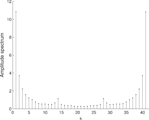
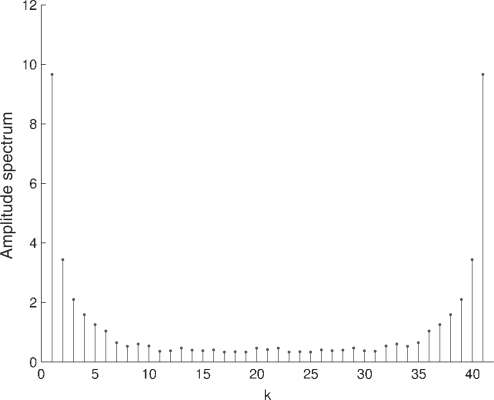
We have used the Discrete Fourier Transform (DFT) to characterize the periodicity observed in the plots of the relative error for the coding regions (Figs. 5 and 6). Figure 7 shows the spectrum of the relative error for the coding regions of the human genome and Figure 8 shows the spectrum of the complete human genome. Figure 7 reveals a local peak at k=N/3, which corresponds to a period of three samples. It is known that the symbolic autocorrelation spectrum of protein coding DNA regions typically has a peak at k=N/3 frequency (Afreixo et al., 2004b; Voss, 1992; Wang and Johnson, 2002). It has been shown in Afreixo et al. (2004a) that the symbolic autocorrelation spectrum and the indicator sequences spectrum are equivalent concepts.

Fig. 7.

Absolute value of the DFT of the relative error in the coding regions of the H.sapiens genome.

Fig. 8.

Absolute value of the DFT of the relative error in the complete genome of H.sapiens.

3.2 Analysis of multiple organisms

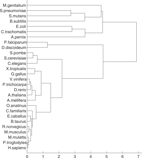
The relative error vectors of each complete genome may be used as a genomic signature that identifies each species, thus allowing the comparison of species. These vectors were used to build dendrograms that show hierarchical clusters which could be interpreted as phylogenetic trees. The dendrograms were built using complete linkage clustering and the similarity matrix was computed using the Euclidean distance.

The hierarchical clustering was applied to a matrix composed by the first 100 distances for all the species used in this study. For the organisms with the smaller genomes, the relative error of the distances that do not occur is set to zero. Figure 9 shows the phylogenetic tree for all the species in this study. The phylogenetic tree of our results (obtained with complete linkage) displays a first branching between prokaryotes and eukaryotes. Apart from the slight misplacement of the archaeota being displayed in-between the bacteria, all other branchings are correct, according to the whole-genome-based tree of Ciccarelli et al. (2006). As for the eukaryotes, the vertebrates are almost all correctly evaluated (the primates are all well clustered), according to Margulies and Birney (2008), except for some obvious misplacements, such as the zebrafish (D.rerio) that is branched with the plants, and the frog (X.tropicalis) and chicken (G.gallus) that are further away from the higher vertebrates than expected.

Fig. 9.

Phylogenetic tree with the species used in this study.

The bacterial subset reveals somewhat longer branches than expected. This may be due to the impact of the small size of the bacteria genome for the purpose of computing inter-nucleotide distances. In fact, it is common that the distance distributions of the bacteria genomes are highly sparse for distances above 50.

4 CONCLUSION

The inter-nucleotide distance mapping characterizes completely a DNA sequence, in the sense of providing a invertible mapping: the original sequence can be reconstructed from the inter-nucleotide distances. The results obtained in this work suggest that for the addressed species there is a genetic signature, a pattern, that is a distinguishing characteristic of that species. The pattern, which is obtained from the distribution of the inter-nucleotide distances, is contained in any of the chromosomes of all species used in this work.

Another interesting feature of the inter-nucleotide approach is the significant similarity found for the A/T and C/G nucleotides. This similarity may be explained by the existence of inverted repeats.

We used the inter-nucleotide distance to build dendrograms that may have a biological interpretation and may be considered as a kind of phylogenetic tree. The dendrograms for the species used in this work are in accordance with the expected similarities between species.

We expect that the inter-nucleotide distance mapping may stimulate further investigations and improve our knowledge about the correlation structure of DNA.

Funding: Fundação para a Ciência e a Tecnologia (FCT); European Social Fund (to S.P.G.); Ministério da Ciência, Tecnologia e Ensino Superior (MCTES, to S.P.G.).

Conflict of Interest: none declared.

REFERENCES

- Afreixo VMA, et al. Fourier analysis of symbolic data: a brief review. Digit. Signal Process. 2004a;14:523–530. [Google Scholar]
- Afreixo VMA, et al. The spectrum and symbol distribution of nucleotide. Phys. Rev. E. 2004b;70:031910. doi: 10.1103/PhysRevE.70.031910. [DOI] [PubMed] [Google Scholar]
- Akhtar M, Epps J. Signal processing in sequence analysis: Advances in eukaryotic gene prediction. IEEE J. Sel. Top. Signal Process. 2008;2:310–321. [Google Scholar]
- Akhtar M, et al. 5th International Workshop on Genomic Signal Processing and Statistics. Tuusula, Finland: 2007. On DNA numerical representation for period-3 based exon prediction. [Google Scholar]
- Anastassiou D. Genomic signal processing. IEEE Signal Process. Mag. 2001;18:8–20. [Google Scholar]
- Brodzik AK, Peters O. Proceedings of IEEE ICASSP. Vol. 5. Philadelphia, PA: IEEE; 2005. Symbol-balanced quaternionic periodicity transform for latent pattern detection in DNA sequences; pp. 373–376. [Google Scholar]
- Buldyrev S, et al. Long-range correlation properties of coding and noncoding DNA sequences: GenBank analysis. Phys. Rev. E. 1995;51:5084–5091. doi: 10.1103/physreve.51.5084. [DOI] [PubMed] [Google Scholar]
- Ciccarelli FD, et al. Toward automatic reconstruction of a highly resolved tree of life. Science. 2006;311:1283–1287. doi: 10.1126/science.1123061. [DOI] [PubMed] [Google Scholar]
- Cristea PD. Large scale features in DNA genomic signals. Signal Process. 2003;83:871–888. [Google Scholar]
- Doggett N. Overview of human repetitive DNA sequences. Curr. Protocols Hum. Genet. 2001 doi: 10.1002/0471142905.hga01bs08. Appendix 1B. Available at http://www.currentprotocols.com/protocol/hga01b. [DOI] [PubMed] [Google Scholar]
- Hodge T, Cope MJTV. A myosin family tree. J. Cell Sci. 2000;113:3353–3354. doi: 10.1242/jcs.113.19.3353. [DOI] [PubMed] [Google Scholar]
- Jeffrey HJ. Chaos game representation of gene structure. Nucleic Acids Res. 1990;18:2163–2170. doi: 10.1093/nar/18.8.2163. [DOI] [PMC free article] [PubMed] [Google Scholar]
- Liao B, et al. Application of 2-d graphical representation of DNA sequence. Chem. Phys. Lett. 2005;401:196–199. [Google Scholar]
- Margulies EH, Birney E. Approaches to comparative sequence analysis: towards a functional view of vertebrate genomes. Nat. Rev. Genet. 2008;9:303–313. doi: 10.1038/nrg2185. [DOI] [PubMed] [Google Scholar]
- Nair ASS, Mahalakshmi T. Proceedings of IEEE Genomic Signal Processing. Romania: Bucharest; 2005. Visualization of genomic data using inter-nucleotide distance signals. [Google Scholar]
- Ning J, et al. Proceedings of IEEE Bioinformatics Conference. Stanford, CA: Ning; 2003. Preliminary wavelet analysis of genomic sequences; pp. 509–510. [Google Scholar]
- Randic M. Another look at the chaos-game representation of DNA. Chem. Phys. Lett. 2008;456:84–88. [Google Scholar]
- Silverman BD, Linsker R. A measure of DNA periodicity. J. Theor. Biol. 1986;118:295–300. doi: 10.1016/s0022-5193(86)80060-1. [DOI] [PubMed] [Google Scholar]
- Voss RF. Evolution of long-rang fractal correlations and 1/f noise in DNA base sequences. Phys. Rev. Lett. 1992;68:3805–3808. doi: 10.1103/PhysRevLett.68.3805. [DOI] [PubMed] [Google Scholar]
- Wang W, Johnson DH. Computing linear transforms of symbolic signals. IEEE Trans. Signal Process. 2002;50:628–634. [Google Scholar]
- Zhang R, Zhang CT. Z curves, an intuitive tool for visualising and analysing the DNA sequences. J. Biomol. Struct. Dyn. 1994;11:767–782. doi: 10.1080/07391102.1994.10508031. [DOI] [PubMed] [Google Scholar]