Visual Receptive Field Structure of Cortical Inhibitory Neurons Revealed by Two-Photon Imaging Guided Recording

Abstract

Synaptic inhibition plays an important role in shaping receptive field (RF) properties in the visual cortex. However, the underlying mechanisms remain not well understood, partly because of difficulties in systematically studying functional properties of cortical inhibitory neurons in vivo. Here, we established two-photon imaging guided cell-attached recordings from genetically labeled inhibitory neurons and nearby “shadowed” excitatory neurons in the primary visual cortex of adult mice. Our results revealed that in layer 2/3, the majority of excitatory neurons exhibited both On and Off spike subfields, with their spatial arrangement varying from being completely segregated to overlapped. In contrast, most layer 4 excitatory neurons exhibited only one discernable subfield. Interestingly, no RF structure with significantly segregated On and Off subfields was observed for layer 2/3 inhibitory neurons of either the fast-spike or regular-spike type. They predominantly possessed overlapped On and Off subfields with a significantly larger size than the excitatory neurons and exhibited much weaker orientation tuning. These results from the mouse visual cortex suggest that different from the push-pull model proposed for simple cells, layer 2/3 simple-type neurons with segregated spike On and Off subfields likely receive spatially overlapped inhibitory On and Off inputs. We propose that the phase-insensitive inhibition can enhance the spatial distinctiveness of On and Off subfields through a gain control mechanism.

Introduction

Since the first description of simple and complex cells in the primary visual cortex (V1) (Hubel and Wiesel, 1962), the synaptic circuits underlying these two types of cells have been studied and discussed extensively. It is generally proposed for simple cells that the spatially segregated On and Off subregions in their receptive fields (RFs) primarily originate from convergent inputs from On- and Off-center thalamic relay cells, respectively (Hubel and Wiesel, 1962; Chapman et al., 1991; Reid and Alonso, 1995; Ferster and Miller, 2000). However, the contribution of cortical input, especially that of cortical inhibitory input, to the generation of simple-cell RFs remains controversial. A popular model proposed to explain the inhibitory contribution is exemplified in a “push-pull” circuit, where a simple cell receives input from cortical interneurons whose RFs mirror that of the simple cell (Ferster and Miller, 2000; Hirsch and Martinez, 2006). This model clearly explains the antagonistic relationship between On and Off response subregions (i.e., in the On subfield, On stimuli increase the cell's firing rate whereas Off stimuli decrease it, and vice versa) (Hubel and Wiesel, 1962; Movshon et al., 1978; Heggelund, 1981; Palmer and Davis, 1981). It is supported by a few intracellular recording studies in cat visual cortex, showing that excitation and inhibition in simple cells were spatially opponent (Ferster, 1988; Hirsch et al., 1998). In addition, orientation selectivity of inhibition in simple cells is usually the same as that of excitation (Anderson et al., 2000; Monier et al., 2003), as expected from the push-pull model.

However, the results contradicting the push-pull model have also been obtained. One intracellular study has suggested that On and Off responses may consist of both excitatory and inhibitory inputs in simple cells (Borg-Graham et al., 1998). Moreover, the extracellular or intracellular blockade of GABA receptors can result in the conversion of the simple-cell RF structure to the complex-cell-like structure (Sillito, 1975; Nelson et al., 1994), implying a spatial overlap between excitation and inhibition. A more recent quantitative study suggests that spike threshold transforms a continuous distribution in the spatial organization of synaptic inputs into two distinct functional classes, simple and complex (Priebe et al., 2004). An implication from this result is that the push-pull may only apply to the “purest” simple cells. These above findings suggest that new circuit features may need to be incorporated into the push-pull model. For example, simple cells may receive input from both orientated, simple-like and nonorientated, complex-like inhibitory neurons (Hirsch et al., 2003) as to achieve contrast-invariant orientation tuning (Troyer et al., 1998; Ferster and Miller, 2000).

It remains a major challenge to clearly dissect visually evoked excitatory and inhibitory synaptic inputs to a cortical neuron in vivo. Complementarily, characterization of RF properties of inhibitory neurons can provide useful information on the inhibitory contribution to functional properties of cortical neurons. Such studies remain limited, however, mainly because of the sparseness of inhibitory neurons. Only 15–20% of cortical neurons are inhibitory (Peters and Kara, 1985; Hendry et al., 1987; Prieto et al., 1994), and they are morphologically and neurochemically diverse (DeFelipe, 1993; Cauli et al., 1997; Kawaguchi and Kubota, 1997; Markram et al., 2004), increasing the level of complexity. Previous studies have mostly focused on neurons exhibiting fast-spiking properties (Azouz et al., 1997; Cardin et al., 2007; Niell and Stryker, 2008; Nowak et al., 2008), a physiological hallmark for parvalbumin-positive inhibitory neurons (Kawaguchi and Kondo, 2002). However, other classes of inhibitory neurons cannot be identified using this method. In addition, because some excitatory neurons also exhibit fast-spiking properties (Dykes et al., 1988; Gray and McCormick, 1996; Swadlow, 2003), potential misclassification should be considered. Intracellular recording combined with staining and morphological reconstruction allows precise identification of inhibitory neurons (Azouz et al., 1997; Hirsch et al., 2003), but with this method it is difficult to sample a large number of cells. Because of the limitations of these methods, a more detailed understanding of functional properties of cortical inhibitory neurons remains to be established.

Transgenic technique provides a solution to efficiently targeting cortical inhibitory neurons. By using cell-type-specific promoters, transgenic mouse lines have been generated in which inhibitory neurons are genetically labeled with green fluorescence protein (GFP) (Oliva et al., 2000; Meyer et al., 2002; Tamamaki et al., 2003; Di Cristo et al., 2004). The mouse visual cortex is potentially a useful model to study neuronal circuitry underlying visual cortical processing, because various fundamental RF properties such as simple/complex RF structure and orientation/direction selectivity are preserved in the mouse V1, despite that the physical size of RFs is considerably larger than that in cats and monkeys (Drager, 1975; Mangini and Pearlman, 1980; Metin et al., 1988; Niell and Stryker, 2008). In addition, specific molecular/genetic manipulations can be readily applied to the mouse cortex, greatly facilitating studies of functional neuronal circuitry.

A Ca²⁺ imaging study on a GAD67-GFP knock-in mouse line suggests that GABAergic neurons exhibit weaker orientation selectivity than non-GABAergic neurons (Sohya et al., 2007). However, the relationship between the change in fluorescence intensity of Ca²⁺ indicators and the level of spike response in cortical neurons, which is likely nonlinear, was not characterized in this study. Considering that some inhibitory neurons have a much higher activity level than excitatory cells (Swadlow, 1989; Azouz et al., 1997), potential saturation of fluorescence signal cannot be overlooked. Another limitation of Ca²⁺ imaging is that because of the slow decay of Ca²⁺ signals, the interval between stimuli has to be long enough to allow individual responses to be resolved. Therefore, it will take a tremendous amount of time to map high-resolution spatial RFs with Ca²⁺ imaging. In this study, a more straightforward approach was used.

In the same GAD67-GFP mouse line, we applied two-photon imaging guided targeted cell-attached recordings to both GFP-positive inhibitory neurons and “shadowed” excitatory neurons in layer 2/3 of the V1, where excitatory cells primarily exhibited segregated or overlapped On and Off subfields. We found that inhibitory neurons, of either the fast-spike (FS) or regular-spike (RS) type, predominantly possessed overlapped On and Off subfields and exhibited weak or no orientation selectivity. These results suggest that the layer 2/3 excitatory neurons with segregated spike On and Off subfields likely receive spatially overlapped inhibitory On and Off inputs. We hypothesize that in the mouse visual cortex, the phase-insensitive inhibitory inputs can enhance the spatial segregation of On and Off subfields through a gain control mechanism.

Materials and Methods

Animal preparation.

The GAD67-GFP (Δneo) mouse line was maintained by crossing heterozygous transgenic females with wild-type C57BL/6 males. This transgenic line was referred to as GAD67-GFP mouse line in this study. The female heterozygous progenies were used for imaging guided recording experiments. The blind loose-patch recordings were performed in female wild-type C57BL/6 mice. All experimental procedures were approved by the Institutional Animal Care and Use Committee at the University of Southern California. Adult mice (3–4 months old) were anesthetized with urethane (1.2 g/kg) and sedative chlorprothixene (0.05 ml of 4 mg/ml), as described previously (Mangini and Pearlman, 1980; Wagor et al., 1980; Metin et al., 1988; Niell and Stryker, 2008). Lactated Ringer's solution was infused intraperitoneally at 3 ml/kg/h to prevent dehydration. The animal's body temperature was maintained at ∼37.5° by a rectal thermoprobe feeding back to a heating pad (Harvard Apparatus). A section of 1.2 mm glass tube was inserted into the trachea to maintain a clear airway. The animal was placed in a custom-built stereotaxic holder. The part of the skull and dura mater (∼0.5 × 0.5 mm) over the primary visual cortex was removed. Artificial CSF solution [ACSF; containing (in mm) 140 NaCl, 2.5 KCl, 2.5 CaCl₂, 1.3 MgSO₄, 1.0 NaH₂PO4, 20 HEPES, 11 glucose, pH 7.4) was applied to the exposed cortical surface when necessary. Throughout the surgical procedure, the lids were sutured to protect the eyes. After the procedure, the lid of the right eye was opened, and drops of 30k silicone oil were applied to prevent it from drying.

In vivo two-photon imaging guided or blind cell-attached loose-patch recording.

In vivo two-photon imaging was performed with a custom-built imaging system (see Fig. 3A). A mode-locked Ti:sapphire laser (Mai Tai Broadband; Spectra-Physics) was tuned to 890 nm, and the laser power through the objective was adjusted within the range of 10–40 mW. In each individual trial, the output power of the laser was kept at a minimum to avoid photo-damage of the cell. Scanning was controlled by a custom-modified scanning software (from Dr. K. Svoboda, Janelia Farm, Ashburn VA). Emission light was collected by a 40× water-immersion objective (numerical aperture 0.8; IR2; Olympus), filtered by an emission filter (HQ515/50; Chroma Technology) and measured by a PMT detector (Hamamatsu R3896). The scanning speed (1–8 ms per line), the zoom factor, and the resolution for each frame (16–1024 pixels) were adjusted in each individual experiment. The V1 was first mapped using extracellular recordings to identify its retinotopic map (Wagor et al., 1980). For cell-attached recording, the glass electrode, with ∼1 μm tip opening and 10–12 MΩ impedance, was filled with ACSF containing 0.15 mm calcein (Invitrogen). The pipette tip was initially guided into V1 region using micromanipulators (model MX7700; Siskiyou) under low-magnification epifluorescence imaging (with 4× objective) and penetrated the pia at a 30° angle. Agar was not applied. Both GFP-labeled neurons and the recording pipette were visualized with a single detection channel. Within 300 μm below the pia, the image quality was good enough for discerning the boundary of the soma as well as the pipette tip. The pipette tip was first brought close to a target cell (within 30 μm away from the cell body in x–y plate and at a z level corresponding to the upper one-third of the target cell body). The tip was then navigated in small zig-zag motions to approach the cell body at its upper one-third position. A holding potential of −40 mV was applied. The current through the pipette and the image of the pipette tip were monitored simultaneously during the pipette navigation. The contact of the pipette tip with the correct cell was judged by the concurrence between the proximity of the pipette tip to the soma and the appearance of large oscillatory currents (at a frequency of the heart beats), as well as the decrease in the leak current (see Fig. 3C). The appearance of oscillatory currents before the pipette tip reached the cell would indicate a false hit. In many experiments, cells were subjected to several attempts of pipette approaching before a correct contact was confirmed. After the confirmation of a successful targeting, the positive pressure in the pipette (∼10 mbar) was then released, and a negative pressure (20–150 mbar) was applied to form a loose seal (with 80–200 MΩ resistance), which was maintained throughout the course of recordings. Spike responses were recorded with an Axopatch 200B amplifier (Molecular Devices). The pipette capacitance was compensated. Loose-patch recordings were made under voltage-clamp mode, and a command potential was adjusted so that the baseline current was 0 pA (Perkins, 2006). The recorded signal was filtered at 10 kHz by a four-pole Bessel low-pass filter of the amplifier and sampled at 20 kHz. Cells recorded under imaging were all located at 120–300 μm below the pia, corresponding to layer 2/3.

Figure 3.

Two-photon imaging guided cell-attached recording. A, Schematic diagram for our customized two-photon imaging system. Red beams indicate the optic pathway of the two-photon laser. The power of the laser beam is controlled by a ½ waveplate coupled with a polarized beam splitter. A PMT coupled with an emission filter wheel allows detection of six different types of fluorescence emission. An epifluorescence imaging system with a CCD camera was incorporated for directly viewing GFP fluorescence (green beam). Excitation (blue beam) was provided by a blue light-emitting diode lamp. Dichroic mirror 1 was designed to switch between two-photon mode (2) and epifluorescence mode (E). B, Top, Two-photon image of V1 in a GAD67-GFP mouse at a depth of ∼150 μm below the pial surface. The arrow points to the tip of the recording pipette, which was filled with ACSF containing calcein. Scale bar, 50 μm. Bottom left, A loose patch was formed on a GFP-positive cell body. The primary dendrites of the target cell could be identified, and the surface of the soma was depressed by the pipette tip. Scale bar, 10 μm. Bottom right, leakage of calcein over time increased fluorescence of the extracellular space, and GFP-negative cell bodies appeared as dark shadows (arrows) that could be targeted as presumptive excitatory neurons. Scale bar, 10 μm. C, Progression of a targeted patch. Left, Images (y-projection) showing progressive movement of the pipette tip toward the target cell. Scale bar, 10 μm. Right, Traces of leak current under −40 mV for the corresponding time point. Note that the proximity of the pipette tip to the cell membrane coincided with the appearance of large oscillatory current changes (III). Additional pressing of the cell by the pipette tip reduced the leak current. D, Example experiment of a targeted whole-cell patch, with the pipette loaded with a red dye (rhodamine B). Top, Image in green channel. Bottom, Superimposed image in both green and red channels. Note that the target cell was stained by the red dye and appeared yellow. The red signal to its left was caused by a blood vessel. Scale bar, 20 μm.

For blind cell-attached loose-patch recordings, glass electrodes with a larger tip opening (5–7 MΩ impedance) were used. With this parameter, all the neurons we recorded showed regular spikes, suggesting that sampling was highly biased toward excitatory neurons (i.e., at least 90% of recorded cells were excitatory). In blind recording experiments in which we attempted to record from FS neurons, pipettes with a smaller tip opening (10–15 MΩ) were used, and in ∼10% of trials, FS neurons were encountered, consistent with the population of fast-spiking inhibitory neurons in the cortex. To determine the laminar location of neurons, histology with Nissl staining of visual cortical sections was performed. Neurons assigned to layer 2/3 in this study were located 100–350 μm beneath the pia, and neurons assigned to layer 4 were at a depth of 375–500 μm. Depth variation of ±25 μm does not affect our conclusion.

Visual stimulation.

Software for data acquisition and visual stimulation was custom developed using LabView (National Instruments). Visual stimuli were provided by a 34.5 × 25.9 cm monitor (refresh rate, 120 Hz; mean luminance, ∼10 cd/m²) placed 25 cm away from the right eye. The center of the monitor was placed at 45° azimuth (corresponding to the monocular zone) and 0° elevation (Wagor et al., 1980), and it covered ±35° horizontally and ±27° vertically of the visual field of the mouse. To map spatial RFs, a set of bright and dark squares over a gray background (contrast of 70 and −70%, respectively) within an 11 × 11 grid (grid size of 2.5–5°, according to the RF size) was flashed individually (duration, 200 ms) in a pseudo-random sequence. Each stimulus was at least five pixels away from the previous one and at least four pixels away from the next previous one. The interstimulus interval was 300 ms to minimize the interference between responses evoked by consecutive stimuli. The sign of contrast (On or Off) was determined randomly. Each location was stimulated 10–20 times, and the same number of On and Off stimuli were applied. The large number of repetitions allowed the collection of a sufficient number of spikes and increased signal/noise ratio. The On and Off subfields were derived from responses to the onset of bright and dark squares, respectively. In some experiments, flashing bright/dark bar stimuli (2–3°) at the preferred orientation were also applied, and the classification of cell types based on the mapping with bars was consistent with mapping with sparse stimuli (10 On-/Off-dominating cells and 12 S-RF/O-RF cells). To measure orientation tuning, drifting square-wave grating of 12 directions (30° step) at an optimal speed (20–40°/s) was presented on the full screen for 2 s with an interstimulus interval of 8 s. The grating started to drift 7 s after it appeared on the screen and stopped drifting for 1 s. Grating of another orientation then appeared immediately. The mean luminance of the screen was thus kept constant. The grating consists of alternating 5° white and 15° black bars, respectively (100% contrast) (Sohya et al., 2007). The 12 patterns were presented in a random sequence and were repeated for 5–10 times. For the measurement of modulation ratios, drifting sinusoidal gratings at the preferred direction (with a temporal frequency of 2 Hz) were presented for 50–100 cycles, at various spatial frequencies (0.01, 0.02, 0.04, 0.08, 0.16, 0.32 cycle/°) (Skottun et al., 1991; Niell and Stryker, 2008). Orientation tuning property tested with sinusoidal gratings was consistent with that tested with square-wave gratings.

Data analysis.

Spikes were detected off-line. To analyze the spike shapes, 50 individual spike waveforms (without filter application) were averaged to calculate the peak–peak interval and P0/P1 ratio. For flashing stimuli, stimulus-evoked spikes were counted within a 70–220 ms time window after the onset of the stimulus in the majority of cells (see supplemental Fig. 1, available at www.jneurosci.org as supplemental material). In a few cells that exhibited shorter onset delays (60–65 ms), the starting time for the 150 ms analysis window was adjusted accordingly. Spikes evoked by drifting gratings were counted within a 70–2000 ms window. The baseline activity (average spike number in the same length of duration before the onset of stimuli) was subtracted from stimulus-evoked spike numbers. Responses with the peak firing rate larger than threefold of SD of baseline activity were considered as significant. The subfield was identified as an area where pixels with significant evoked responses were spatially contiguous.

To quantify the separation between On and Off subfields, an overlap index (OI) (Schiller et al., 1976; Hirsch and Martinez, 2006) was calculated for cells exhibiting both On and Off subfields. The OI is defined as follows:

where d is the distance between the centers of two ellipses and W₁ and W₂ are the widths of them, respectively, which are the segments of the line that connects the two centers intercepted by the ellipses. To determine d and W, we first fit the spike On and Off subfields separately with a two-dimensional elliptical Gaussian:

where A determines the maximum amplitude, a and b are half-axes of the ellipse, and x′ and y′ are transformations of the stimulus coordinates x and y, taking into account of the angle θ and the coordinates of the center (xc, yc) of the ellipse. Thus, there are six free parameters in the fitting procedure: A, a, b, θ, xc, and yc. We did not force θ to be the same for the On and Off fields, because this sometimes introduced a significant mismatch of the shape of one subfield with its fitted shape. The outline of the ellipse was determined as such that it could cross as many pixels at the boundary of RF as possible. OI approaches 1 when the two fields are overlapped symmetrically. OI is ≤0 when the two fields are completely separated. For cells with more than two subfields, the OI of the cell was calculated as the average of OI values for each pair of adjacent subfields.

To quantitatively describe the spatial relationship between On and Off responses without fitting of subfields, Pearson's correlation coefficient (Priebe et al., 2004; Mata and Ringach, 2005) was calculated according to the following equation:

where R_on,i and R_off,i are individual responses to On and Off stimuli, respectively. R̄_on and R̄_off are the mean On and Off response within the subfield, respectively. Only the pixels for which either On or Off response was significant above the baseline were considered in calculating r.

The strength of orientation selectivity was quantified in three ways. In the first, the responses to drifting gratings of two directions at each orientation were averaged to obtain the orientation tuning curve between 0 and 180°, which was then fitted with Gaussian function R(θ) = A*exp(−0.5*(θ − ϕ)²/σ²) + B. ϕ is the preferred orientation, and σ controls the tuning width. The orientation selectivity index (OSI) is defined as (R_pref − R_orth)/(R_pref + R_orth) = A/(A + 2*B), where R_pref is the response level at angle of ϕ, and R_orth is that at an angle of ϕ + 90°. In the second, we quantified the tuning curve as the half-bandwidth at half-maximum of the Gaussian fit above the nontuned component (Schiller et al., 1976). When the tuning curve was too flat to fit, we arbitrarily chose the maximum response as R_pref, the response at 90° away from the angle of the maximum response as R_orth, and 90° as the tuning width. In the third, we used a global measure of orientation selectivity (Chapman and Stryker, 1993; Dragoi et al., 2000; Sohya et al., 2007):

θ_i is the angle of the moving direction of the grating. R(θ_i) is the spike response amplitude at angle θ_i. This measurement combines aspects of both the depth of modulation and tuning width into one value.

The modulation ratio M = R(F₁)/R(F₀) was calculated for responses to gratings at optimal spatial frequency. The peristimulus spike-time histogram (PSTH) was first generated from all the cycles. R(F₁) was calculated from the PSTH as the amplitude of the best-fitting sinusoid at the modulation frequency (Ringach et al., 2002). R(F₀) was the mean spike rate during the drifting grating stimulus. Spontaneous activity was subtracted when calculating the modulation ratio.

Post hoc analyses were used to identify differences among groups. The Tamhane T2 multiple comparison test was used because it does not assume equal sample sizes or variances.

Results

Layer 2/3 excitatory neurons mostly exhibit RFs with segregated or overlapped On and Off subregions

To provide a reference for responses properties of inhibitory neurons, we first examined RF properties of excitatory neurons by applying blind loose-patch recordings (see Materials and Methods) in layers 2–4 of wild-type mice. Previous results on the RF properties of excitatory neurons in the mouse V1 had appeared inconsistent. Some early studies showed that simple- and complex-cell RFs primarily appeared in layer 2/3, whereas layer 4 neurons mostly exhibited On-center or Off-center RFs (Mangini and Pearlman, 1980; Metin et al., 1988). A more recent study based on responses to sinusoidal gratings concluded that the majority of layer 4 neurons were simple cells (Niell and Stryker, 2008). This inconsistency could be attributable to the different methods used in defining RF types. In this study, we mapped the On and Off subregions of visual RFs with sparse flashing stimuli. The stimuli contained bright and dark squares flashed in a pseudo-random sequence within a 11 × 11 array, which covered the entire RF of the cell (see Materials and Methods). Spike responses to each unit stimulus were displayed with a PSTH. Spiking activity significantly above the baseline level in response to the flashing stimuli could be detected for the majority of neurons. Based on the spatial arrangement of On and Off subregions, RFs of layer 2–4 neurons could be roughly categorized into three types. Typical examples of RF types are shown in Figure 1. The cell in Figure 1A exhibited a spatially distinct On subregion (the visual space where bright stimuli significantly increase spiking activity) and Off subregion (the space where dark stimuli increase spiking). We call this type of RF “S-RF” (i.e., receptive field with segregated On and Off subfields). S-RF cells usually responded to drifting sinusoidal gratings with strongly modulated responses (Fig. 1A, right). The cell in Figure 1B exhibited largely overlapped On and Off subregions. We call this type of cell “O-RF” cell. The cell in Figure 1C exhibited only one subfield under spot stimuli. Mapping with flashing oriented bars also revealed only one subfield (Fig. 1C, bottom). We call the cells with one dominating subfield “On-dominating” or “Off-dominating” cells. The majority of these types of cells also exhibited strongly modulated responses to sinusoidal gratings (Fig. 1C, right; supplemental Fig. 2A, available at www.jneurosci.org as supplemental material).

Figure 1.

Spike RF structures of presumptive excitatory neurons in the V1 of wild-type mice. A, An example S-RF cell. B, An O-RF cell. C, An On-dominating cell. Left, An example spike waveform. The dotted line marks the position of the peak. Calibration: horizontal, 1 ms; vertical, 88 pA (A), 48 pA (B), 25 pA (C). Middle left, On and Off responses to all the stimuli. The trace in each pixel represents the PSTH for spike responses (generated from all the trials) to a unit On or Off stimulus at the corresponding location. Each pixel represents visual space of 4° (A), 5° (B), and 4° (C). Red and blue ovals depict the two-dimensional Gaussian fit of the On and Off subfield, respectively. Calibration: horizontal, 200 ms; vertical, 14 Hz (A), 22 Hz (B), 23 Hz (C). Middle right, Superimposed color maps for spike On (red) and Off (green) responses. The brightness of the colors represents the evoked firing rate. The maps were smoothed by bilinear interpolation. The one-dimensional map below the square color map in C represents superimposed On and Off responses to flashing bars of the preferred orientation (indicated by the white bar) at various locations. The brightest color represents 13.7 Hz. Note that there was no Off response. Right, PSTH of spike responses evoked by the drifting sinusoidal grating at optimal spatial frequency within one cycle. The modulation ratio is 1.2 (A), 0.33 (B), or 1.67 (C). D, Gaussian fits of On (red) and Off (blue) subfields for the population of excitatory neurons, grouped according to their laminar locations and RF types. Scale bar, 10°. L2/3, Layer 2/3; L4, layer 4. E, Histogram of strength ratio between the maximum On and maximum Off response within the identified RF. The ratio was derived by dividing the smaller value by the larger value. Most On- or Off-dominating cells had no response to one sign of contrast.

To quantitatively describe RF structures, discernible On or Off subfields were fitted with two-dimensional Gaussian eclipses (see Materials and Methods). RF outlines for the population of blindly recorded excitatory neurons were plotted and grouped according to their laminar locations and RF structures (Fig. 1D). In layer 4, only a small number of neurons (27%) exhibited both On and Off subfields. The majority of layer 4 neurons (73%) exhibited On- or Off-dominating RFs. Consistent with previous findings (Drager, 1975; Metin et al., 1988), more On-dominating cells were observed than Off-dominating cells. On- or Off-dominating cells mostly did not show spike responses to the other contrast, or only exhibited extremely weak responses (Fig. 1E). Three RFs possessed responses to the opposite contrast surrounding the dominating subfield (see supplemental Fig. 2B, available at www.jneurosci.org as supplemental material), reminiscent of the center-surround structure. In contrast, in layer 2/3, the majority of neurons (73%) exhibited both On and Off subfields, with their spatial arrangement varying from being completely segregated to overlapped, consistent with previous hand mapping experiments (Mangini and Pearlman, 1980; Metin et al., 1988). The relative strength between On and Off subfields varied (Fig. 1E). The prevalence of On- or Off-dominating RFs in layer 4, but not in layer 2/3 of the mouse V1, suggests that layer 4 neurons primarily receive major excitatory input from either On-center or Off-center thalamic relay neurons (Grubb and Thompson, 2003; Van Hooser et al., 2003), whereas there is more robust convergence of On and Off information in layer 4 to layer 2/3 projections.

To classify S-RF and O-RF cells in a quantitative way, we quantified the spatial relationship between On and Off subfields with an OI as well as Pearson's correlation coefficient (see Materials and Methods) (Fig. 2A,B). We found that these two independent measures exhibited a strong linear correlation (r = 0.95) (Fig. 2A). An OI of 0.3 approximately corresponds to a correlation coefficient of 0, which separates cells into two functional groups in cat and macaque V1 (Priebe et al., 2004; Mata and Ringach, 2005). In the histogram of OI values for the population of excitatory neurons, OI 0.3 also clearly separated cells into two groups (Fig. 2B). Based on these data, we set OI 0.3 as a boundary between S-RF and O-RF cells. On the other hand, the relative modulation of responses to drifting sinusoidal gratings (modulation ratio, F₁/F₀), a widely used functional measure to distinguish simple and complex cells (Skottun et al., 1991), correlated less well with the OI or the correlation coefficient (Fig. 2C,D). For example, some cells with OI >0.5 exhibited strong response modulation (with a modulation ratio >1), yet they might be more appropriately classified as “complex” cells based on the subfield overlap. When considering modulation ratio only, there are more simple cells than complex cells in layer 2/3, which is, in fact, consistent with the recent report in the mouse V1 (Niell and Stryker, 2008). Our results are reminiscent of a study in awake monkeys, which showed that some V1 neurons with overlapping On and Off activation regions exhibited strongly modulated responses to sinusoidal gratings (Kagan et al., 2002). To avoid confounds, in this study we classified cells into S-RF and O-RF cells solely based on the spatial arrangement of their subfields.

Figure 2.

Relationship between OI, correlation coefficient, and modulation ratio of excitatory neurons. A, Plot of correlation coefficient (r) against OI. Each data point represents values obtained in the same cell. The red line is the best-fit linear regression line. Dashed lines mark OI 0.3 and r = 0, respectively. Note that these two measures give similar grouping results. B, Histogram of OI for the population of excitatory neurons exhibiting both On and Off subfields. The dashed line marks OI 0.3. C, Plot of modulation ratio (F₁/F₀) against OI. The red line is the best-fit linear regression line. r = −0.69. The dashed line marks OI 0.3 and F₁/F₀ = 1 (which separates simple from complex cells), respectively. Note that cells in space b will be grouped differently according to different measures. D, Plot of modulation ratio against correlation coefficient. r = −0.60.

Two-photon imaging guided cell-attached recording

Since excitatory neurons in layer 2/3 primarily possess RFs with segregated or overlapped On and Off subfields, and the major inhibitory input to these neurons comes from inhibitory neurons in the same layer (Dantzker and Callaway, 2000; Yoshimura and Callaway, 2005; Yoshimura et al., 2005), investigating RF structures of layer 2/3 inhibitory neurons will provide insight into the inhibitory mechanism underlying the On/Off RF structures. In this study, we developed the two-photon imaging guided patch-clamp recording (TPTP) technique (Margrie et al., 2003) to directly record from genetically labeled inhibitory neurons. A GAD67-GFP knock-in mouse line (Tamamaki et al., 2003) was exploited. As reported previously, essentially all GFP-positive neurons are GABAergic in this line (Tamamaki et al., 2003). We have built a customized two-photon imaging system (Fig. 3A) to perform visually guided loose-patch recording from fluorescence-labeled neurons. Under our two-photon excitation microscope, GFP-positive cell bodies were observed to disperse across the visual cortex (Fig. 3B, top). Fluorescent cell bodies could be imaged as deep as 400 μm below the pial surface. In TPTP, the glass electrode, which was filled with ACSF containing the bright-green fluorescent dye calcein (150 μm), was navigated under visual guidance to patch onto a selected fluorescent soma (Fig. 3B, bottom left) (see Materials and Methods). Dye leakage from the recording pipette, together with the diffuse fluorescence from the mesh of labeled axons and dendrites, could result in a relatively high background, over which GFP-negative cell bodies appeared dark (Fig. 3B, bottom right). By targeting these shadowed cell bodies (Kitamura et al., 2008), we could also record from excitatory neurons identified by their spontaneous spiking activity. We developed a protocol to ensure the correctness of targeting by simultaneously monitoring the relative position of the pipette tip to the target cell body and the leak current through the pipette (see Materials and Methods). When the correct cell was contacted, the proximity of the pipette tip to the target cell, the appearance of large oscillatory current changes (likely caused by the pulsation of the cortex), and the decrease in the leak current occurred at the same time (Fig. 3C). The reliability of our method was proven by a few experiments in which a whole cell was formed after targeted patch and the target cell was stained by the dye of a different color contained in the pipette (Fig. 3D).

In the cell-attached recording, spikes of the target cell were detected with a high signal/noise ratio (Fig. 4A). According to spike shape, we further categorized GFP-positive inhibitory neurons into two groups: FS and RS inhibitory neurons. FS neurons (25 of 50) had spikes with short peak–peak intervals (0.32 ± 0.04 ms; mean ± SD), whereas RS inhibitory neurons (25 of 50) had spikes with longer peak–peak intervals (0.91 ± 0.08 ms) (Fig. 4A,C). Spikes of the FS neurons tend to have larger P0/P1 ratios, the ratio of the amplitude of the peak to that of the trough, than those of the RS neurons (Fig. 4A,C). The peak–peak interval and P0/P1 ratio have been used previously to characterize spike shape (Andermann et al., 2004; Barthó et al., 2004; Hasenstaub et al., 2005; Mitchell et al., 2007; Wu et al., 2008). Under loose-patch condition, spike shape was relatively insensitive to changes in seal resistance during recordings (Fig. 4B) (Perkins, 2006). The spiking property of FS neurons was consistent with that of parvalbumin-positive inhibitory neurons, which occupy about half of the inhibitory neuron population in the cortex (Gonchar and Burkhalter, 1997; Kawaguchi and Kondo, 2002). The GFP-positive RS neurons may represent nonparvalbumin-positive inhibitory cell classes. As a comparison, all the excitatory neurons we recorded exhibited regular spikes (Fig. 4C). On average, inhibitory neurons of both FS and RS types had a higher level of spontaneous spiking activity than excitatory neurons (Fig. 4D). FS neurons also responded to visual stimuli at a significantly higher firing rate than excitatory neurons (Fig. 4D), consistent with previous reports (Swadlow, 1989; Azouz et al., 1997). It is worth noting that excitatory and RS inhibitory neurons cannot be reliably distinguished simply based on firing rate and spike shape, since there is a large overlap of these measures between the two groups (supplemental Fig. 3, available at www.jneurosci.org as supplemental material). The application of the TPTP technique in the GAD67-GFP mice thus enabled us to systematically investigate different neuronal types at least in the superficial layers of the cortex.

Figure 4.

TPTP identified three neuronal types. A, Left, Example traces of recorded spikes from a GFP(+) FS neuron (top) and a GFP(+) RS neuron (bottom), evoked by a bright square displayed for 200 ms (top trace). Right, Spike shape for four example FS neurons (top) and RS neurons (bottom). For each cell, 50 individual spikes (black) and their average (red) were superimposed. Dotted lines mark the trough and the peak, the amplitudes of which are represented by P1 and P0, respectively. The peak–peak interval was measured between the two dashed lines. Note that fast spikes are characterized by a relatively larger P0 and relatively shorter peak–peak interval. Calibration: horizontal, 1 ms; vertical, 30, 24, 80, and 50 pA (top) and 60, 36, 50, and 70 pA (bottom). B, An example experiment showing that spike shape remained relatively stable as seal resistance changed. Spike shapes were shown for different time points during the recording. Calibration: horizontal, 1 ms; vertical, 36, 60, and 80 pA (from top to bottom). C, Scatter plot of P0/P1 ratio versus peak–peak (P-P) interval for the identified inhibitory and excitatory neurons. The dotted line indicates the boundary between FS and RS cells. GFP(+) and GFP(−) neurons were marked in green and black, respectively. D, Average firing rate (spontaneous and evoked) for the three groups of neurons. For evoked response, the strongest response in RF mapping was used. Error bars indicate SE. *p < 0.05, Tamhane T2 multiple comparison test. n = 21, 20, and 20 for GFP(+) FS, GFP(+) RS, and GFP(−) RS neurons, respectively.

Layer 2/3 inhibitory neurons predominantly possess overlapped On and Off subfields

We next examined RF structures of inhibitory neurons in layer 2/3. To map the On and Off subfields of inhibitory neurons, the same sparse stimuli were applied. As shown in Figure 5A, for an example of a GFP-positive FS neuron, its On and Off subfields were similar in size and shape and were almost completely overlapped with each other. For an example of a GFP-negative excitatory neuron recorded, the On and Off subfields were primarily spatially separated, and the size of subfields was smaller (Fig. 5B). Spatial RFs of 41 inhibitory neurons (GFP+) and 20 excitatory neurons (GFP−) in layer 2/3 of 22 GAD67-GFP mice were reconstructed. Among them, six inhibitory (three FS and three RS) and three excitatory neurons exhibited On- or Off-dominating RFs. For the other cells exhibiting both On and Off subfields, their fitted RFs were plotted in Figure 5C. For all the FS inhibitory neurons, the On and Off fields were almost completely overlapped, sometimes with one larger subfield covering the other smaller one. The OI values were mostly close to 1 (Fig. 5C, left). For the RS inhibitory neurons, their On and Off subfields also tended to be largely overlapped with each other, despite some variation (Fig. 5C, middle). In contrast, excitatory neurons exhibited a much broader variation in their RF structures. Some cells showed clearly segregated subfields with OI values close to 0, and others had typical O-RFs with largely overlapped subfields (Fig. 5C, right). Statistical analysis indicated that there was a significant difference in the distribution of OI (Fig. 5D) between the excitatory neurons and the FS or RS inhibitory neurons [p < 0.001, Tamhane T2 multiple comparison test; n = 18, 17, and 17 for GFP(+) FS, GFP(+) RS, and GFP(−) RS neurons, respectively]. Consistent with the OI analysis, inhibitory neurons exhibited a higher spatial correlation between the On and Off subfields than excitatory neurons (Fig. 5D). Additionally, the subfield size of the FS or RS inhibitory neurons was significantly larger than that of the excitatory neurons (Fig. 5E). The average subfield size was 24.3 ± 4.6, 22.6 ± 5.5, and 14.4 ± 2.9 (mean ± SD) degrees for the FS, RS inhibitory, and excitatory neurons, respectively. Inhibitory neurons, on average, exhibited weaker modulation in their responses to drifting sinusoid gratings (Fig. 5F). Together, these data demonstrated that in layer 2/3 there is significantly more spatial overlap between On and Off subfields in the population of inhibitory neurons than excitatory neurons.

Figure 5.

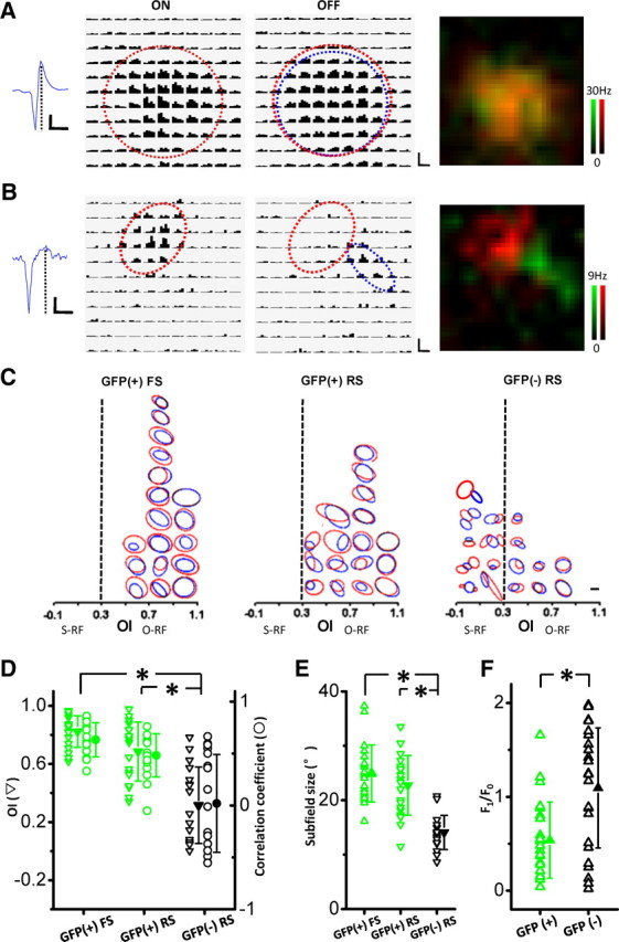
Spike RF structures of identified excitatory and inhibitory neurons in layer 2/3. A, B, Spike RFs of an example GFP(+) inhibitory neuron (A) and a GFP(−) excitatory neuron (B). Plotting is similar to that in Figure 1A. Left, Traces of example spike waveforms. Calibration: horizontal, 1 ms; vertical, 100 pA (A) and 60 pA (B). Middle, PSTH for On and Off responses to all the stimuli. Red and blue ovals depict the Gaussian fits of the On and Off subfields, respectively. Each pixel represents 5° in visual space. Calibration: horizontal, 200 ms; vertical, 36 Hz (A) and 16 Hz (B). Right, Superimposed color maps for On (red) and Off (green) responses. C, Outlines of Gaussian fits of spike On and Off subfields for the three types of neurons. Red and blue ovals represent On and Off subfields, respectively. RFs were binned according to their OI values. Bin size, 0.2. Scale bar, 10°. D, Distribution of OI (triangle) and correlation coefficient (circle) for different groups of neurons. n = 18, 17, and 17 for GFP(+) FS, GFP(+) RS, and GFP(−) RS neurons, respectively. *p < 0.001, Tamhane T2 multiple comparison test. E, Distribution of subfield size. For S-RF and O-RF cells, subfield size was the average of On and Off subregions. n = 21, 20, and 20 for GFP(+) FS, GFP(+) RS, and GFP(−) RS neurons, respectively. *p < 0.001. F, Distribution of modulation ratio. n = 25 and 24 for GFP(+) and GFP(−) neurons, respectively. *p < 0.001, t test. Solid symbols indicate mean value, and error bars indicate SD.

Layer 2/3 inhibitory neurons exhibit weak or no orientation selectivity

The push-pull model requires that simple-cell-like, orientation selective inhibitory neurons exist. Such kind of inhibitory neurons have been found in layer 4 of the cat V1 (Hirsch et al., 2003). In contrast, a subset of complex-like inhibitory neurons was reported untuned to orientation (Hirsch et al., 2003; Nowak et al., 2008). Here, we also examined orientation tuning profiles of inhibitory and excitatory neurons in the mouse V1. Moving gratings at 12 directions (30° step for 360° visual space) were applied 5–10 times for each cell (see Materials and Methods). As shown in Figure 6A, the example excitatory neuron exhibited strong spike responses only to a small range of orientations. In contrast, the example FS inhibitory neuron responded similarly to gratings at all orientations. More examples as shown in the polar graphs in Figure 6B indicated a significant difference in tuning profile between excitatory and inhibitory neurons. We quantified the degree of orientation tuning using three measures (see Materials and Methods): (1) OSI, which is derived from the responses to the preferred and orthogonal orientations; (2) tuning width, which is half-bandwidth at half-maximum of the tuning function; and (3) global OSI, which is a global measure of tuning curve combining aspects of both the depth of modulation and tuning width. Figure 6C–E plots the distributions of these three measures for the three types of neurons. FS and RS inhibitory neurons mostly had low OSI values, indicating that they were not tuned or only weakly tuned to orientation. Excitatory neurons exhibited a broad range of OSI values, from nonselective to highly selective (Fig. 6C). Inhibitory neurons also showed broader tuning widths than excitatory neurons (Fig. 6D). The difference in tuning profile between excitatory and inhibitory neurons was magnified when the global OSI was measured (p < 0.001, Tamhane T2 multiple comparison test) (Fig. 6E). This difference cannot be simply attributed to the large subfield overlap in inhibitory neurons, since excitatory neurons with similar OIs can exhibit much sharper orientation selectivity (Fig. 6F). Together, our data demonstrated that compared with excitatory neurons, inhibitory neurons have much lower sensitivity to stimulus orientation, which is consistent with the results of the Ca²⁺ imaging experiment (Sohya et al., 2007). This result agrees with the models that inhibition can contribute to the sharpening of orientation selectivity through its broad, nonselective tuning (Ben-Yishai et al., 1995; Somers et al., 1995; McLaughlin et al., 2000; Ringach et al., 2003).

Figure 6.

Orientation tuning of identified inhibitory and excitatory neurons in layer 2/3. A, Spike responses to moving gratings of 12 directions in an example GFP(−) RS excitatory neuron (Ex.) and a GFP(+) FS inhibitory neuron (In.). Blue traces are recorded spike responses (in one trial) under each drifting grating. The corresponding PSTH for each orientation (5 repeats) is plotted below. B, Polar plots of visual responses for six cells. Numbers in parentheses represent the axial scale, the average number of spikes evoked after baseline subtraction. The first two inhibitory neurons (In.) were FS neurons, and the third was a RS neuron. C, Distribution of OSI for the three groups of neurons. n = 22, 15, and 33 for GFP(+) FS, GFP(+) RS, and GFP(−) RS neurons, respectively. *p < 0.001, Tamhane T2 multiple comparison test. D, Distribution of tuning width. *p < 0.05. E, Distribution of global OSI. *p < 0.001. F, Plot of OSI versus OI. Excitatory neurons include GFP(−) neurons in TPTP experiments and those recorded blindly in wild-type mice. Solid symbols indicate mean value, and error bars indicate SD.

Discussion

Genetic labeling provides a useful tool for targeted examination of sparse cell types. In this study, we exploited an existing GAD67-GFP mouse line, in which almost all the GABAergic neurons are labeled (Tamamaki et al., 2003). By applying TPTP, we examined the RF properties of inhibitory and excitatory neurons specifically in layer 2/3 of the V1. We found significant differences between these two types of neurons (i.e., inhibitory neurons have broader subfields, less spatial separation between On and Off subfields, and weaker orientation selectivity than excitatory neurons). There are two possibilities that can explain these differences between inhibitory and excitatory neurons. First, inhibitory neurons may receive a broader range of synaptic inputs. For example, since apparent orientation columns are absent in rodent visual cortex (Ohki et al., 2005), inhibitory neurons may receive input promiscuously from other cells with different orientation tunings, whereas connections made between excitatory neurons may be more specific such that connected cells have similar tuning properties. Second, inhibitory neurons may receive similar ranges of synaptic inputs; however, they may be more efficient in transforming synaptic inputs to spike outputs. More efficient transformation has been observed in some FS neurons in cat visual cortex (Cardin et al., 2007) and rat auditory cortex (Wu et al., 2008). Both the level of spike threshold and membrane biophysical properties (e.g., input resistance and membrane time constant) can contribute to the transformation efficiency. To distinguish these possibilities, further investigations by applying targeted intracellular recordings are needed.

GAD67-GFP transgenic line

One concern about the transgenic line used in this study is that one copy of GAD67 gene has been deleted because of the targeted introduction of GFP gene (Tamamaki et al., 2003). GABA content in the transgenic brain is reduced in the first few weeks after birth (Tamamaki et al., 2003), which may affect the maturation of inhibitory synapses (Chattopadhyaya et al., 2007). However, it is apparently normal in the adult brain, possibly being compensated by other factors such as GAD65 (Tamamaki et al., 2003). In addition, no apparent physical or behavioral abnormalities have been observed for adult GAD67-GFP mice (Tamamaki et al., 2003; our observations). We also compared the identified layer 2/3 excitatory neurons in transgenic mice and the RS excitatory neurons recorded blindly in wild-type mice. We did not find any significant difference in various RF properties, such as spatial separation between On and Off subfields, subfield size, and orientation tuning between transgenic mice and wild-type mice (p > 0.5) (Fig. 7). Furthermore, FS neurons recorded blindly in layer 2/3 of wild-type mice (see Materials and Methods) also exhibited similar average OI and subfield size (OI: 0.77 ± 0.13, n = 8; subfield size: 23 ± 7.5°, n = 10; mean ± SD) as the FS neurons recorded in the transgenic mice (OI, 0.82 ± 0.11; subfield size, 25 ± 5°; p > 0.6, t test) (Fig. 5D,E). These results demonstrate that there is no significant difference in RF properties between wild-type and adult transgenic mice. Thus, it is reasonable to believe that the RF properties of GFP-positive neurons in the GAD67-GFP transgenic line reflect general features of cortical inhibitory neurons in the mouse visual cortex.

Figure 7.

Comparison of RF properties of excitatory neurons between the transgenic and wild-type mice. A, Distribution of OI. n = 17 and 25 (from left to right). p = 0.61, t test. B, Distribution of subfield size. n = 20 and 37. p = 0.87. C, Distribution of global OSI. n = 33 and 33. p = 0.65.

Inhibitory cell types

Inhibitory neurons in the cortex are neurochemically and electrophysiologically diverse. Some major types of inhibitory neurons have been well characterized in in vitro studies (Kawaguchi and Kondo, 2002; Markram et al., 2004; Somogyi and Klausberger, 2005). In this study, according to spike shape, we could categorize the recorded GABAergic neurons into two types, FS and RS. The spike shape of FS neurons, especially the short peak–peak interval, suggests that this type of inhibitory neuron is the same as the fast-spiking neuron reported in many previous studies (McCormick et al., 1985; Connors and Kriegstein, 1986). Fast-spiking neurons are parvalbumin positive and include two morphological types, basket cell and chandelier cell (Kawaguchi and Kondo, 2002; Markram et al., 2004). Parvalbumin-positive neurons constitute ∼50% of the total GABAergic cells in the cortex, and in layer 2/3, they account for ∼37% of GABAergic neurons (Gonchar and Burkhalter, 1997). In our TPTP study, the FS neurons constitute 50% of the total recorded inhibitory neurons. On one hand, this proportion suggests that there was a slight bias toward FS cells in our sampling of inhibitory neurons, possibly because of relatively stronger fluorescence labeling of these cells. On the other hand, this proportion has greatly supported the specificity of our targeted recording, since errors in targeting would significantly increase the proportion of cells with RS property. The FS neurons are most likely parvalbumin-positive basket cells, because much more sparsely distributed chandelier cells (which also exhibit fast spikes) may not be driven by sensory input under normal physiological conditions (Zhu et al., 2004). The recorded RS neurons may include somatostatin-positive bitufted and calretinin-positive biopolar or bitufted cells (Reyes et al., 1998; Thomson and Morris, 2002; Thomson et al., 2002; Markram et al., 2004).

Implication on inhibitory inputs

The laminar distribution of RF structure in mouse V1 appears to be different from that of the cat. In mouse V1, RFs with segregated On and Off subfields mostly appear in the superficial layers, whereas simple cells in cat V1 dominate the thalamorecipient layers (Martinez et al., 2005). This laminar distribution suggests that S-RFs in layer 2/3 are primarily formed by a convergence of inputs from On- and Off-dominating cells in layer 4. In the meantime, inhibitory inputs to the S-RF cells may shape their spike RF structure. As demonstrated previously in rodent visual cortical slices, the majority of layer 2/3 pyramidal neurons (86%, 12 of 14) receive major inhibitory input (>80%) from local inhibitory neurons in the same layer (Dantzker and Callaway, 2000; Yoshimura and Callaway, 2005; Yoshimura et al., 2005). Only a small percentage of layer 2/3 pyramidal neurons (14%, 2 of 14) receive a significant portion of inhibitory input (∼50%) from layer 4 (Dantzker and Callaway, 2000). Because layer 2/3 inhibitory neurons are predominantly O-RF cells, the majority of layer 2/3 pyramidal neurons should receive spatially overlapped inhibitory On and Off inputs from these inhibitory neurons.

Since FS neurons dominate inhibitory neuron population in layer 4 (Gonchar and Burkhalter, 1997) and provide some inhibitory input to upper layers (Thomson and Morris, 2002; Thomson et al., 2002), we also examined RF structures of layer 4 FS neurons by blind loose-patch recordings. Consistent with layer 2/3, no S-RF structure was observed for these neurons. They exhibited either O-RFs or On-/Off-dominating RFs (see supplemental Fig. 4, available at www.jneurosci.org as supplemental material). Although convergence of inputs from On- and Off-dominating layer 4 FS neurons can possibly result in spatially segregated inhibitory On and Off inputs in layer 2/3 neurons, this is unlikely a major synaptic mechanism underlying S-RF structure, since the proportion of S-RF cells is much higher than that of cells receiving significant inhibitory input from layer 4 (Fig. 1D). Thus, our results suggest that layer 2/3 pyramidal cells even with segregated spike On and Off subfields likely receive spatially overlapped inhibitory On and Off inputs.

Intracellular studies in the cat V1 suggest that simple cells possess spatially opponent excitatory and inhibitory inputs (Ferster, 1988; Hirsch et al., 1998), which has been the basis for the push-pull circuit model in explaining the simple-cell RF structure. The model requires that inhibitory neurons providing the opponent inhibition be simple-cell like, and it predicts that these neurons are tuned to orientation. Consistent with this model, it has been found that simple-cell-like, orientation-tuned inhibitory neurons exist in layer 4 of the cat V1 (Hirsch et al., 2003) and that inhibitory input to simple cells usually has the same tuning as excitatory input (Anderson et al., 2000; Monier et al., 2003). Interestingly, in the mouse V1, we have not found inhibitory neurons with simple-cell-like RFs. They predominantly possess overlapped On and Off subfields and are hardly orientation selective. This suggests that push-pull cannot be a major synaptic mechanism underlying S-RFs in mouse V1 and inhibitory circuits may contribute in a different way to the formation of simple-cell-like RFs.

How might spatially overlapped On and Off inhibitory inputs contribute to the segregation of spike On and Off subfields? Because of the large subfield size of inhibitory neurons (Fig. 5E) as well as the retinotopic organization of synaptic connections, inhibitory and excitatory inputs to S-RF cells likely have substantial spatial overlap. This potential overlap has also been implicated by several studies (Sillito, 1975; Nelson et al., 1994; Borg-Graham et al., 1998; Yoshimura and Callaway, 2005). It then allows a spatiotemporal interaction between excitatory and inhibitory inputs. A previous study has shown that the nonlinear mechanism of spike threshold can enhance the functional differences between simple and complex cells (Preibe et al., 2004). By generally suppressing membrane excitation, which is equivalent to elevating spike threshold, spatially overlapped On and Off inhibition can increase the separation between spike subfields when excitatory On and Off inputs are already partially segregated. Thus, similar to the models that broadly tuned inhibition can sharpen response selectivity (Somers et al., 1995; McLaughlin et al., 2000; Wu et al., 2008), the phase-insensitive inhibitory inputs can sharpen the spatial discreteness of spike On and Off subfields of visual cortical neurons.

Altogether, our results in mouse V1 suggest that a push-pull circuit may not be required for the formation of a simple-cell-like RF structure. The nonselective inhibition may contribute to the selectivity of excitatory neurons through a gain control mechanism.

References

- Andermann ML, Ritt J, Neimark MA, Moore CI. Neural correlates of vibrissa resonance; band-pass and somatotopic representation of high-frequency stimuli. Neuron. 2004;42:451–463. doi: 10.1016/s0896-6273(04)00198-9. [DOI] [PubMed] [Google Scholar]
- Anderson JS, Carandini M, Ferster D. Orientation tuning of input conductance, excitation, and inhibition in cat primary visual cortex. J Neurophysiol. 2000;84:909–926. doi: 10.1152/jn.2000.84.2.909. [DOI] [PubMed] [Google Scholar]
- Azouz R, Gray CM, Nowak LG, McCormick DA. Physiological properties of inhibitory interneurons in cat striate cortex. Cereb Cortex. 1997;7:534–545. doi: 10.1093/cercor/7.6.534. [DOI] [PubMed] [Google Scholar]
- Barthó P, Hirase H, Monconduit L, Zugaro M, Harris KD, Buzsáki G. Characterization of neocortical principal cells and interneurons by network interactions and extracellular features. J Neurophysiol. 2004;92:600–608. doi: 10.1152/jn.01170.2003. [DOI] [PubMed] [Google Scholar]
- Ben-Yishai R, Bar-Or RL, Sompolinsky H. Theory of orientation tuning in visual cortex. Proc Natl Acad Sci U S A. 1995;92:3844–3888. doi: 10.1073/pnas.92.9.3844. [DOI] [PMC free article] [PubMed] [Google Scholar]
- Borg-Graham LJ, Monier C, Frégnac Y. Visual input evokes transient and strong shunting inhibition in visual cortical neurons. Nature. 1998;393:369–373. doi: 10.1038/30735. [DOI] [PubMed] [Google Scholar]
- Cardin JA, Palmer LA, Contreras D. Stimulus feature selectivity in excitatory and inhibitory neurons in primary visual cortex. J Neurosci. 2007;27:10333–10344. doi: 10.1523/JNEUROSCI.1692-07.2007. [DOI] [PMC free article] [PubMed] [Google Scholar]
- Cauli B, Audinat E, Lambolez B, Angulo MC, Ropert N, Tsuzuki K, Hestrin S, Rossier J. Molecular and physiological diversity of cortical nonpyramidal cells. J Neurosci. 1997;17:3894–3906. doi: 10.1523/JNEUROSCI.17-10-03894.1997. [DOI] [PMC free article] [PubMed] [Google Scholar]
- Chapman B, Stryker MP. Development of orientation selectivity in ferret visual cortex and effects of deprivation. J Neurosci. 1993;13:5251–5262. doi: 10.1523/JNEUROSCI.13-12-05251.1993. [DOI] [PMC free article] [PubMed] [Google Scholar]
- Chapman B, Zahs KR, Stryker MP. Relation of cortical cell orientation selectivity to alignment of receptive fields of the geniculocortical afferents that arborize within a single orientation column in ferret visual cortex. J Neurosci. 1991;11:1347–1358. doi: 10.1523/JNEUROSCI.11-05-01347.1991. [DOI] [PMC free article] [PubMed] [Google Scholar]
- Chattopadhyaya B, Di Cristo G, Wu CZ, Knott G, Kuhlman S, Fu Y, Palmiter RD, Huang ZJ. GAD67-mediated GABA synthesis and signaling regulate inhibitory synaptic innervation in the visual cortex. Neuron. 2007;54:889–903. doi: 10.1016/j.neuron.2007.05.015. [DOI] [PMC free article] [PubMed] [Google Scholar]
- Connors BW, Kriegstein AR. Cellular physiology of the turtle visual cortex: distinctive properties of pyramidal and stellate neurons. J Neurosci. 1986;6:164–177. doi: 10.1523/JNEUROSCI.06-01-00164.1986. [DOI] [PMC free article] [PubMed] [Google Scholar]
- Dantzker JL, Callaway EM. Laminar sources of synaptic input to cortical inhibitory interneurons and pyramidal neurons. Nat Neurosci. 2000;3:701–707. doi: 10.1038/76656. [DOI] [PubMed] [Google Scholar]
- DeFelipe J. Neocortical neuronal diversity: chemical heterogeneity revealed by colocalization studies of classic neurotransmitters, neuropeptides, calcium-binding proteins, and cell surface molecules. Cereb Cortex. 1993;4:273–289. doi: 10.1093/cercor/3.4.273. [DOI] [PubMed] [Google Scholar]
- Di Cristo G, Wu C, Chattopadhyaya B, Ango F, Knott G, Welker E, Svoboda K, Huang ZJ. Subcellular domain-restricted GABAergic innervation in primary visual cortex in the absence of sensory and thalamic inputs. Nat Neurosci. 2004;7:1184–1186. doi: 10.1038/nn1334. [DOI] [PubMed] [Google Scholar]
- Drager UC. Receptive fields of single cells and topography in mouse visual cortex. J Comp Neurol. 1975;160:269–290. doi: 10.1002/cne.901600302. [DOI] [PubMed] [Google Scholar]
- Dragoi V, Sharma J, Sur M. Adaptation-induced plasticity of orientation tuning in adult visual cortex. Neuron. 2000;28:287–298. doi: 10.1016/s0896-6273(00)00103-3. [DOI] [PubMed] [Google Scholar]
- Dykes RW, Lamour Y, Diadori P, Landry P, Dutar P. Somatosensory cortical neurons with an identifiable electrophysiological signature. Brain Res. 1988;441:45–58. doi: 10.1016/0006-8993(88)91382-0. [DOI] [PubMed] [Google Scholar]
- Ferster D. Spatially opponent excitation and inhibition in simple cells of the cat visual cortex. J Neurosci. 1988;8:1172–1180. doi: 10.1523/JNEUROSCI.08-04-01172.1988. [DOI] [PMC free article] [PubMed] [Google Scholar]
- Ferster D, Miller KD. Neural mechanisms of orientation selectivity in the visual cortex. Annu Rev Neurosci. 2000;23:441–471. doi: 10.1146/annurev.neuro.23.1.441. [DOI] [PubMed] [Google Scholar]
- Gonchar Y, Burkhalter A. Three distinct families of GABAergic neurons in rat visual cortex. Cereb Cortex. 1997;7:347–358. doi: 10.1093/cercor/7.4.347. [DOI] [PubMed] [Google Scholar]
- Gray CM, McCormick DA. Chattering cells: superficial pyramidal neurons contributing to the generation of synchronous oscillations in the visual cortex. Science. 1996;274:109–113. doi: 10.1126/science.274.5284.109. [DOI] [PubMed] [Google Scholar]
- Grubb MS, Thompson ID. Quantitative characterization of visual response properties in the mouse dorsal lateral geniculate nucleus. J Neurophysiol. 2003;90:3594–3607. doi: 10.1152/jn.00699.2003. [DOI] [PubMed] [Google Scholar]
- Hasenstaub A, Shu Y, Haider B, Kraushaar U, Duque A, McCormick DA. Inhibitory postsynaptic potentials carry synchronized frequency information in active cortical networks. Neuron. 2005;47:423–435. doi: 10.1016/j.neuron.2005.06.016. [DOI] [PubMed] [Google Scholar]
- Heggelund P. Receptive field organization of simple cells in cat striate cortex. Exp Brain Res. 1981;42:89–98. doi: 10.1007/BF00235733. [DOI] [PubMed] [Google Scholar]
- Hendry SH, Schwark HD, Jones EG, Yan J. Numbers and proportions of GABA-immunoreactive neurons in different areas of monkey cerebral cortex. J Neurosci. 1987;7:1503–1519. doi: 10.1523/JNEUROSCI.07-05-01503.1987. [DOI] [PMC free article] [PubMed] [Google Scholar]
- Hirsch JA, Martinez LM. Circuits that build visual cortical receptive fields. Trends Neurosci. 2006;29:30–39. doi: 10.1016/j.tins.2005.11.001. [DOI] [PubMed] [Google Scholar]
- Hirsch JA, Alonso JM, Reid RC, Martinez LM. Synaptic integration in striate cortical simple cells. J Neurosci. 1998;18:9517–9528. doi: 10.1523/JNEUROSCI.18-22-09517.1998. [DOI] [PMC free article] [PubMed] [Google Scholar]
- Hirsch JA, Martinez LM, Pillai C, Alonso JM, Wang Q, Sommer FT. Functionally distinct inhibitory neurons at the first stage of visual cortical processing. Nat Neurosci. 2003;6:1300–1308. doi: 10.1038/nn1152. [DOI] [PubMed] [Google Scholar]
- Hubel DH, Wiesel TN. Receptive fields, binocular interaction and functional architecture in the cat's visual cortex. J Physiol. 1962;160:106–154. doi: 10.1113/jphysiol.1962.sp006837. [DOI] [PMC free article] [PubMed] [Google Scholar]
- Kagan I, Gur M, Snodderly DM. Spatial organization of receptive fields of V1 neurons of alert monkeys: comparison with responses to gratings. J Neurophysiol. 2002;88:2557–2574. doi: 10.1152/jn.00858.2001. [DOI] [PubMed] [Google Scholar]
- Kawaguchi Y, Kondo S. Parvalbumin, somatostatin and cholecystokinin as chemical markers for specific GABAergic interneuron types in the rat frontal cortex. J Neurocytol. 2002;31:277–287. doi: 10.1023/a:1024126110356. [DOI] [PubMed] [Google Scholar]
- Kawaguchi Y, Kubota Y. GABAergic cell subtypes and their synaptic connections in rat frontal cortex. Cereb Cortex. 1997;7:476–486. doi: 10.1093/cercor/7.6.476. [DOI] [PubMed] [Google Scholar]
- Kitamura K, Judkewitz B, Kano M, Denk W, Häusser M. Targeted patch-clamp recordings and single-cell electroporation of unlabeled neurons in vivo. Nat Methods. 2008;5:61–67. doi: 10.1038/nmeth1150. [DOI] [PubMed] [Google Scholar]
- Mangini NJ, Pearlman AL. Laminar distribution of receptive field properties in the primary visual cortex of the mouse. J Comp Neurol. 1980;193:203–222. doi: 10.1002/cne.901930114. [DOI] [PubMed] [Google Scholar]
- Margrie TW, Meyer AH, Caputi A, Monyer H, Hasan MT, Schaefer AT, Denk W, Brecht M. Targeted whole-cell recordings in the mammalian brain in vivo. Neuron. 2003;39:911–918. doi: 10.1016/j.neuron.2003.08.012. [DOI] [PubMed] [Google Scholar]
- Markram H, Toledo-Rodriguez M, Wang Y, Gupta A, Silberberg G, Wu C. Interneurons of the neocortical inhibitory system. Nat Rev Neurosci. 2004;5:793–807. doi: 10.1038/nrn1519. [DOI] [PubMed] [Google Scholar]
- Martinez LM, Wang Q, Reid RC, Pillai C, Alonso JM, Sommer FT, Hirsch JA. Receptive field structure varies with layer in the primary visual cortex. Nat Neurosci. 2005;8:372–379. doi: 10.1038/nn1404. [DOI] [PMC free article] [PubMed] [Google Scholar]
- Mata ML, Ringach DL. Spatial overlap of ON and OFF subregions and its relation to response modulation ratio in macaque primary visual cortex. J Neurophysiol. 2005;93:919–928. doi: 10.1152/jn.00668.2004. [DOI] [PubMed] [Google Scholar]
- McCormick DA, Connors BW, Lighthall JW, Prince DA. Comparative electrophysiology of pyramidal and sparsely spiny stellate neurons of the neocortex. J Neurophysiol. 1985;54:782–806. doi: 10.1152/jn.1985.54.4.782. [DOI] [PubMed] [Google Scholar]
- McLaughlin D, Shapley R, Shelley M, Wielaard DJ. A neuronal network model of macaque primary visual cortex (V1): orientation selectivity and dynamics in the input layer 4Calpha. Proc Natl Acad Sci U S A. 2000;97:8087–8092. doi: 10.1073/pnas.110135097. [DOI] [PMC free article] [PubMed] [Google Scholar]
- Metin C, Godement P, Imbert M. The primary visual cortex in the mouse: receptive field properties and functional organization. Exp Brain Res. 1988;69:594–612. doi: 10.1007/BF00247312. [DOI] [PubMed] [Google Scholar]
- Meyer AH, Katona I, Blatow M, Rozov A, Monyer H. In vivo labeling of parvalbumin-positive interneurons and analysis of electrical coupling in identified neurons. J Neurosci. 2002;22:7055–7064. doi: 10.1523/JNEUROSCI.22-16-07055.2002. [DOI] [PMC free article] [PubMed] [Google Scholar]
- Mitchell JF, Sundberg KA, Reynolds JH. Differential attention-dependent response modulation across cell classes in macaque visual area V4. Neuron. 2007;55:131–141. doi: 10.1016/j.neuron.2007.06.018. [DOI] [PubMed] [Google Scholar]
- Monier C, Chavane F, Baudot P, Graham LJ, Frégnac Y. Orientation and direction selectivity of synaptic inputs in visual cortical neurons: a diversity of combinations produces spike tuning. Neuron. 2003;37:663–680. doi: 10.1016/s0896-6273(03)00064-3. [DOI] [PubMed] [Google Scholar]
- Movshon JA, Thompson ID, Tolhurst DJ. Spatial summation in the receptive fields of simple cells in the cat's striate cortex. J Physiol. 1978;283:53–77. doi: 10.1113/jphysiol.1978.sp012488. [DOI] [PMC free article] [PubMed] [Google Scholar]
- Nelson S, Toth L, Sheth B, Sur M. Orientation selectivity of cortical neurons during intracellular blockade of inhibition. Science. 1994;265:774–777. doi: 10.1126/science.8047882. [DOI] [PubMed] [Google Scholar]
- Niell CM, Stryker MP. Highly selective receptive fields in mouse visual cortex. J Neurosci. 2008;28:7520–7536. doi: 10.1523/JNEUROSCI.0623-08.2008. [DOI] [PMC free article] [PubMed] [Google Scholar]
- Nowak LG, Sanchez-Vives MV, McCormick DA. Lack of orientation and direction selectivity in a subgroup of fast-spiking inhibitory interneurons: cellular and synaptic mechanisms and comparison with other electrophysiological cell types. Cereb Cortex. 2008;18:1058–1078. doi: 10.1093/cercor/bhm137. [DOI] [PMC free article] [PubMed] [Google Scholar]
- Ohki K, Chung S, Ch'ng YH, Kara P, Reid RC. Functional imaging with cellular resolution reveals precise micro-architecture in visual cortex. Nature. 2005;433:597–603. doi: 10.1038/nature03274. [DOI] [PubMed] [Google Scholar]
- Oliva AA, Jr, Jiang M, Lam T, Smith KL, Swann JW. Novel hippocampal interneuronal subtypes identified using transgenic mice that express green fluorescent protein in GABAergic interneurons. J Neurosci. 2000;20:3354–3368. doi: 10.1523/JNEUROSCI.20-09-03354.2000. [DOI] [PMC free article] [PubMed] [Google Scholar]
- Palmer LA, Davis TL. Receptive-field structure in cat striate cortex. J Neurophysiol. 1981;46:260–276. doi: 10.1152/jn.1981.46.2.260. [DOI] [PubMed] [Google Scholar]
- Perkins KL. Cell-attached voltage-clamp and current-clamp recording stimulation techniques in brain slices. J Neurosci Methods. 2006;154:1–18. doi: 10.1016/j.jneumeth.2006.02.010. [DOI] [PMC free article] [PubMed] [Google Scholar]
- Peters A, Kara DA. The neuronal composition of area 17 of rat visual cortex. II. The nonpyramidal cells. J Comp Neurol. 1985;234:242–263. doi: 10.1002/cne.902340209. [DOI] [PubMed] [Google Scholar]
- Priebe NJ, Mechler F, Carandini M, Ferster D. The contribution of spike threshold to the dichotomy of cortical simple and complex cells. Nat Neurosci. 2004;7:1113–1122. doi: 10.1038/nn1310. [DOI] [PMC free article] [PubMed] [Google Scholar]
- Prieto JJ, Peterson BA, Winer JA. Morphology and spatial distribution of GABAergic neurons in cat primary auditory cortex (AI) J Comp Neurol. 1994;344:349–382. doi: 10.1002/cne.903440304. [DOI] [PubMed] [Google Scholar]
- Reid RC, Alonso JM. Specificity of monosynaptic connections from thalamus to visual cortex. Nature. 1995;378:281–284. doi: 10.1038/378281a0. [DOI] [PubMed] [Google Scholar]
- Reyes A, Lujan R, Rozov A, Burnashev N, Somogyi P, Sakmann B. Target-cell-specific facilitation and depression in neocortical circuits. Nat Neurosci. 1998;1:279–285. doi: 10.1038/1092. [DOI] [PubMed] [Google Scholar]
- Ringach DL, Shapley RM, Hawken MJ. Orientation selectivity in macaque V1: diversity and laminar dependence. J Neurosci. 2002;22:5639–5651. doi: 10.1523/JNEUROSCI.22-13-05639.2002. [DOI] [PMC free article] [PubMed] [Google Scholar]
- Ringach DL, Hawken MJ, Shapley R. Dynamics of orientation tuning in macaque V1: the role of global and tuned suppression. J Neurophysiol. 2003;90:342–352. doi: 10.1152/jn.01018.2002. [DOI] [PubMed] [Google Scholar]
- Schiller PH, Finlay BL, Volman SF. Quantitative studies of single-cell properties in monkey striate cortex. I. Spatiotemporal organization of receptive fields. J Neurophysiol. 1976;39:1288–1319. doi: 10.1152/jn.1976.39.6.1288. [DOI] [PubMed] [Google Scholar]
- Sillito AM. The contribution of inhibitory mechanisms to the receptive field properties of neurones in the striate cortex of the cat. J Physiol. 1975;250:305–329. doi: 10.1113/jphysiol.1975.sp011056. [DOI] [PMC free article] [PubMed] [Google Scholar]
- Skottun BC, De Valois RL, Grosof DH, Movshon JA, Albrecht DG, Bonds AB. Classifying simple and complex cells on the basis of response modulation. Vision Res. 1991;31:1079–1086. doi: 10.1016/0042-6989(91)90033-2. [DOI] [PubMed] [Google Scholar]
- Sohya K, Kameyama K, Yanagawa Y, Obata K, Tsumoto T. GABAergic neurons are less selective to stimulus orientation than excitatory neurons in layer II/III of visual cortex, as revealed by in vivo functional Ca2+ imaging in transgenic mice. J Neurosci. 2007;27:2145–2149. doi: 10.1523/JNEUROSCI.4641-06.2007. [DOI] [PMC free article] [PubMed] [Google Scholar]
- Somers DC, Nelson SB, Sur M. An emergent model of orientation selectivity in cat visual cortical simple cells. J Neurosci. 1995;15:5448–5465. doi: 10.1523/JNEUROSCI.15-08-05448.1995. [DOI] [PMC free article] [PubMed] [Google Scholar]
- Somogyi P, Klausberger T. Defined types of cortical interneurone structure space and spike timing in the hippocampus. J Physiol. 2005;562:9–26. doi: 10.1113/jphysiol.2004.078915. [DOI] [PMC free article] [PubMed] [Google Scholar]
- Swadlow HA. Efferent neurons and suspected interneurons in S-1 vibrissa cortex of the awake rabbit: receptive fields and axonal properties. J Neurophysiol. 1989;62:288–308. doi: 10.1152/jn.1989.62.1.288. [DOI] [PubMed] [Google Scholar]
- Swadlow HA. Fast-spike interneurons and feedforward inhibition in awake sensory neocortex. Cereb Cortex. 2003;13:25–32. doi: 10.1093/cercor/13.1.25. [DOI] [PubMed] [Google Scholar]
- Tamamaki N, Yanagawa Y, Tomioka R, Miyazaki J, Obata K, Kaneko T. Green fluorescent protein expression and colocalization with calretinin, parvalbumin, and somatostatin in the GAD67-GFP knock-in mouse. J Comp Neurol. 2003;467:60–79. doi: 10.1002/cne.10905. [DOI] [PubMed] [Google Scholar]
- Thomson AM, Morris OT. Selectivity in the inter-laminar connections made by neocortical neurones. J Neurocytol. 2002;31:239–246. doi: 10.1023/a:1024117908539. [DOI] [PubMed] [Google Scholar]
- Thomson AM, Bannister AP, Mercer A, Morris OT. Target and temporal pattern selection at neocortical synapses. Philos Trans R Soc Lond B Biol Sci. 2002;357:1781–1791. doi: 10.1098/rstb.2002.1163. [DOI] [PMC free article] [PubMed] [Google Scholar]
- Troyer TW, Krukowski AE, Priebe NJ, Miller KD. Contrast-invariant orientation tuning in cat visual cortex: thalamocortical input tuning and correlation-based intracortical connectivity. J Neurosci. 1998;18:5908–5927. doi: 10.1523/JNEUROSCI.18-15-05908.1998. [DOI] [PMC free article] [PubMed] [Google Scholar]
- Van Hooser SD, Heimel JA, Nelson SB. Receptive field properties and laminar organization of lateral geniculate nucleus in the gray squirrel (Sciurus carolinensis) J Neurophysiol. 2003;90:3398–3418. doi: 10.1152/jn.00474.2003. [DOI] [PubMed] [Google Scholar]
- Wagor E, Mangini NJ, Pearlman AL. Retinotopic organization of striate and extrastriate visual cortex in the mouse. J Comp Neurol. 1980;193:187–202. doi: 10.1002/cne.901930113. [DOI] [PubMed] [Google Scholar]
- Wu GK, Arbuckle R, Liu BH, Tao HW, Zhang LI. Lateral sharpening of cortical frequency tuning by approximately balanced inhibition. Neuron. 2008;58:132–143. doi: 10.1016/j.neuron.2008.01.035. [DOI] [PMC free article] [PubMed] [Google Scholar]
- Yoshimura Y, Callaway EM. Fine-scale specificity of cortical networks depends on inhibitory cell type and connectivity. Nat Neurosci. 2005;8:1552–1559. doi: 10.1038/nn1565. [DOI] [PubMed] [Google Scholar]
- Yoshimura Y, Dantzker JL, Callaway EM. Excitatory cortical neurons form fine-scale functional networks. Nature. 2005;433:868–873. doi: 10.1038/nature03252. [DOI] [PubMed] [Google Scholar]
- Zhu Y, Stornetta RL, Zhu JJ. Chandelier cells control excessive cortical excitation: characteristics of whisker-evoked synaptic responses of layer 2/3 nonpyramidal and pyramidal neurons. J Neurosci. 2004;24:5101–5108. doi: 10.1523/JNEUROSCI.0544-04.2004. [DOI] [PMC free article] [PubMed] [Google Scholar]