The First Genetic and Comparative Map of White Lupin (Lupinus albus L.): Identification of QTLs for Anthracnose Resistance and Flowering Time, and a Locus for Alkaloid Content

Abstract

We report the first genetic linkage map of white lupin (Lupinus albus L.). An F8 recombinant inbred line population developed from Kiev mutant × P27174 was mapped with 220 amplified fragment length polymorphism and 105 gene-based markers. The genetic map consists of 28 main linkage groups (LGs) that varied in length from 22.7 cM to 246.5 cM and spanned a total length of 2951 cM. There were seven additional pairs and 15 unlinked markers, and 12.8% of markers showed segregation distortion at P < 0.05. Syntenic relationships between Medicago truncatula and L. albus were complex. Forty-five orthologous markers that mapped between M. truncatula and L. albus identified 17 small syntenic blocks, and each M. truncatula chromosome aligned to between one and six syntenic blocks in L. albus. Genetic mapping of three important traits: anthracnose resistance, flowering time, and alkaloid content allowed loci governing these traits to be defined. Two quantitative trait loci (QTLs) with significant effects were identified for anthracnose resistance on LG4 and LG17, and two QTLs were detected for flowering time on the top of LG1 and LG3. Alkaloid content was mapped as a Mendelian trait to LG11.

1. Introduction

Lupinus is a genus of self- or cross-pollinating, mostly indeterminate plant species native to diverse geographic regions.^1,2 Lupins are considered to be polyploid in origin and are found in both the New and Old Worlds. Old World species exhibit different basic chromosome numbers,³ a large variation in the number of their chromosomes, and a 2.5-fold variation in their estimated 2C DNA values.⁴ They are subdivided into the Scabrispermae (rough-seeded) and the Malacospermae (smooth-seeded) to which white lupin (Lupinus albus L.) belongs in conjunction with two other cultivated species: L. angustifolius and L. luteus. White lupin has a diploid chromosome number of 50 and a 2C DNA content of 1.16 ± 0.044 pg.⁴

Lupin species have a relatively short domestication history compared with most crops. Focused breeding efforts began in Germany during World War I due to a need for high-protein pulse crops adapted to temperate conditions. Subsequent breeding has concentrated on the introduction of key traits such as early flowering, reduced pod-shattering, soft seed, and anthracnose disease resistance.^5,6 Lupin grain is high in protein (30–40%) and like soybean is high in dietary fibre (30%), low in oil (6%), and contains minimal starch. Lupin has the lowest Glycaemic Index of any commonly consumed grain (www.glycemicindex.com), which has significant implications for Western societies with an increasing incidence of obesity and associated risk of diabetes and cardiovascular disease.⁷ Lupin fibre acts as a soluble fibre and drops total cholesterol levels without affecting beneficial HDL cholesterol.⁸

White lupin itself is used as feed for livestock and has established a growing market for human consumption due to the development of low alkaloid varieties with a lack of protease inhibitors.^9,10 In addition, white lupin has become an illuminating model for the study of plant adaptation to extreme phosphorus (P) deficiency.^11,12 Adaptation to low P is linked to modifications of root development and biochemistry resulting in proteoid (or cluster) roots.^13–15

Comparative genetic mapping has been studied in many families of crops such as cereals and crucifers,^16–19 and also in legumes.^20–22 More recently, the first comparative map in Lupinus was developed between L. angustifolius and the model legume Medicago truncatula,²³ and subsequently a preliminary comparison was reported between L. albus and M. truncatula.²⁴

Initial comparative mapping studies predominantly used common enzymes, morphological markers, and RFLP probes.^25,26 These have been superseded by PCR-based codominant marker systems that have markedly increased the efficiency and reduced the cost of transferring genetic information across species. In this approach, oligonucleotide primers are designed from sequences of conserved regions such as gene exons that span polymorphic introns or microsatellites to produce ITAPs (intron targeted amplified polymorphic sequence). Examples include the comparison of Medicago truncatula with alfalfa, chickpea, faba bean, narrow-leafed lupin, and pea.^23,27–32

To date only a preliminary genetic map showing three linkage groups (LGs) has been published for white lupin.²⁴ The aims of this study were (1) to construct a complete genetic map of L. albus using orthologous gene-based codominant markers and amplified fragment length polymorphism (AFLP)³³ markers, as a resource for comparing lupin genomes and in legume evolution studies; (2) to map key agronomic traits including anthracnose resistance, low alkaloid content, and flowering time; and (3) to assess the extent of conserved synteny between L. albus and the model legume M. truncatula.

2. Materials and methods

2.1. Genetic mapping population

One hundred and ninety-five F8-derived recombinant inbred lines (RILs) were used to phenotype traits. This population was developed from a cross between cv. Kiev Mutant and an Ethiopian landrace P27174. Kiev Mutant was bred by Dr V.I. Golovchenko of the Ukrainian Agricultural Research Institute, Kiev and was first released in the USSR in 1969. Kiev Mutant was first introduced into Australia by CSIRO in 1972 and subsequently released by the Western Australian Department of Agriculture and Food in 1982. This variety has low alkaloid content and is early flowering but is highly susceptible to anthracnose. P27174 has high alkaloid levels (<1%), is late flowering, and is resistant to anthracnose disease.

To produce the RIL population, Kiev Mutant was used as the female parent and P27174 as the male. The F8 RIL population was primarily made to identify molecular markers linked to anthracnose resistance genes, but variation also exists for other traits such as flowering time, alkaloid content, plant height, pod shape, order of podding, branching, leaf colour and size, brown markings on stems and yield. Only the first three characters were phenotyped for this study. From the 195 F8 RILs, a subset of 94 was randomly chosen for comparative mapping. Total genomic DNA was extracted as previously described by Ellwood et al.³⁴

2.2. Anthracnose resistance phenotyping

The F8 lines were tested against anthracnose from 2004 to 2005 in a disease nursery. The nursery was established in a high rainfall site at Medina, Western Australia, and supplemented with irrigation as required. Spreader rows consisting of a mixture of the susceptible cvs. Kiev Mutant, Wodjil, and Myallie were planted a week before the test lines. The whole population consisting of 195 RILs together with parental controls were planted in 2 m long rows in three replicates between the spreader rows. The test rows were perpendicular to the spreader rows to enable flow of the disease inoculum from both sides. After 3–4 weeks of planting, glasshouse infected Kiev Mutant seedlings were transplanted into the spreader rows at approximately 1 m spacing to ensure a high level of early inoculum. The disease was assessed twice during the season employing a score of 1–5, where 1 is highly resistant and 5 is extremely susceptible. The second, usually higher, scores were used to determine the resistance level of a line.

2.3. Flowering time

Flowering time of F8 RILs was recorded when 50% plants in a test row had one open flower with an erect standard petal on the main stem inflorescence. Due to a large variation in flowering times among lines, the flowering time for each line was recorded in weeks, rather than days, relative to the earliest flowering parent Kiev Mutant. For example, lines that flowered as early as Kiev Mutant were categorized into week 1.

2.4. Alkaloid content

The F8 lines were scored for alkaloid content using two techniques, the Dragendorff paper test and by ultra violet (UV) fluorescence. Pink discolouration of Dragendorff paper indicated high alkaloid content and a white or bleached discolouration indicated no or low alkaloids. Tests were conducted using sap from the petiole of a young leaflet from seedlings at the 8–9 leaf-stage. Similarly, after harvesting seeds were viewed under an UV lamp (Vilber Lourmat, France) at 365 nm. Seeds with a high alkaloid content are fluorescent pink under UV light, whereas those with low alkaloids levels are dull whitish.

2.5. Gene-based PCR markers

Six hundred and twenty-six genic markers belonging to three sets of ITAP primers were utilized in this study.²⁷ These were composed of three sets of ITAPs; the ‘ML’ primers, that were developed from alignment between M. truncatula and Lupinus spp. EST sequences.²³ A small proportion of these markers were designed to span microsatellite motifs rather than introns; the ‘MLG’ primers were designed from alignment of M. truncatula, L. albus, and Glycine max EST sequences;²⁷ and the cross-species ‘MP’ markers developed at the Department of Plant Pathology, University of California, Davis, USA.²⁰ The majority of the ITAP primers were from genes in characterized chromosomal regions, and therefore the L. albus mapped markers could be physically mapped in M. truncatula using M. truncatula BACs.

2.6. Polymorphism detection

Each primer pair was screened on L. albus parental DNA.²³ Single PCR products of the same size were purified and directly sequenced. DNA polymorphisms were identified by manual inspection of alignments and chromatograms using Vector NTI (Invitrogen, Carlsbad, California). Different procedures were used to genotype the F8 population depending on types of polymorphism identified.²⁷

2.7. AFLP markers

AFLP markers were generated as described by Nelson et al.²³ and Vos et al.,³³ using one selective nucleotide for pre-amplification (EcoRI-C and MseI-A) and two selective nucleotides for selective amplification. The AFLP products were resolved with an AB3730 DNA Sequencer using a GeneScan™ -500 LIZ^® Size Standard [Applied Biosystems (AB), Foster City, California, USA]. Data were analysed by the automated allele calling parameters in GeneMapper^® (AB). Marker nomenclature included the name of selective marker combination; either A or B depending on whether inherited from Kiev mutant or P27274, respectively; and the marker size (in bp).

2.8. Genetic, comparative, and QTL mapping

Ninety-four F8 RILs were scored for polymorphic gene-based and AFLP molecular markers together with three agronomic traits (anthracnose resistance, alkaloid, and flowering time). Genetic linkage mapping was conducted with MultiPoint v. 1.2 software (MultiQTL Ltd, Institute of Evolution, Haifa University, Israel). The Kosambi mapping function was used to convert the recombination frequencies into genetic distance (cM). Chi-square analysis (P < 0.05) was applied to test the segregation of the mapped markers against the expected Mendelian segregation ratio for codominant inheritance in an F8 RIL population. Groups of linked markers that were similarly distorted were accepted for linkage mapping and QTL analysis. Independent markers showing significant segregation distortion and markers with missing data (>10%) were rejected for linkage and QTL analysis to avoid bias and false linkages.

Markers mapped in L. albus were located on the M. truncatula map by aligning marker EST template sequences using BLASTN to phases 1, 2 and 3 sequenced BACs (Build 17.06.06, http://www.medicago.org/). Alignments with a BLAST E-values < 1 × 10⁻²⁰, hsp identity ≥ 60%, and hsp length > 50 nt were retained.

Association between each LG and the putative QTL regions related to flowering time and anthracnose resistance were determined by interval mapping using MultiQTL software, version 2.5 (MultiQTL Ltd, Institute of Evolution, Haifa University, Israel). Significance levels for each QTL detected were determined with 1000 permutations and the standard deviation (SD) for each QTL determined by 1000 Bootstraps. Analysis of variance (ANOVA) using JMP-IN 5.1 (SAS Institute, Cary, NC) was also used to determine correlation between markers flanking each QTL and the corresponding trait. All QTLs identified were further confirmed with MapManager QTX v. b20.³⁵

3. Results and discussion

3.1. General features of the first L. albus genetic linkage map

A total of 325 markers consisting of 105 genic markers and 220 AFLP markers were used to generate the first comprehensive genetic linkage map for L. albus. Amplicon sequences have been submitted to Genbank under accession codes EI394666, EI394667, and EI392791–EI392938.

The multilocus AFLPs were employed to generate sufficient markers to coalesce the LGs described by gene-based markers. This was necessary due to the large number of chromosomes in L. albus, (n = 25),⁴ and the tendency of conserved genes as genic markers to cluster in isolated blocks.³⁶ Genic markers were chosen to enable syntenic relationships between L. albus and the model legume species, M. truncatula, to be established.

Table 1 and Fig. 1 summarize general properties of the map. The map comprised 28 LGs, that varied in length from 246.5 to 22.7 cM and the total map length was 2951 cM. The average spacing between markers was 12.6 cM, determined at a recombination fraction (rf) of 0.27. In addition, there were seven pairs of linked markers. Unique placements within LGs could not be determined for 25 markers and 15 markers remained unlinked. Ambiguous markers positioning in Multipoint v. 1.2 may occur due to missing data, miss-genotyping, or rare recombination events that push out the length of the chromosome. The first two occurred in this study and are the result of residual heterozygosity in F8 lines. Thus, before mapping, ‘H's are removed from the data for co-dominant markers, while the dominant nature of AFLPs disguises otherwise co-dominant loci. Genic markers were evenly distributed throughout the genome with the exceptions of LGs 9, 14, and 28 which were composed only of AFLP markers. Only two examples of markers mapped to multiple loci occurred in this study: LSSR16 and LSSR33. Unlike RFLPs, ITAPs are limited in their ability to detect duplications. Exceptions occur when two or more amplicons for a given marker are of different lengths but share similar amplification intensities and are individually polymorphic between the parents.

Table 1.

Properties of the first genetic map of L. albus

Linkage group	Length (cM)	Number of polymorphic markers	Number of defined locia	Average marker spacing (cM)	Associated trait
LG1	246.5	26	19	9.9	Flowering time
LG2	255.1	21	15	13.4	Nil
LG3	116.1	20	15	7.7	Flowering time
LG4	144.2	18	16	8.5	Anthracnose resistance
LG5	161.6	17	12	14.7	Nil
LG6	125.6	16	13	10.5	Nil
LG7	102.4	14	13	8.5	Nil
LG8	194.3	14	13	16.2	Nil
LG9	139.0	13	10	13.9	Nil
LG10	131	12	12	11.9	Nil
LG11	157.1	12	11	15.7	Alkaloid content
LG12	95.1	10	9	11.9	Nil
LG13	116.7	10	9	14.6	Nil
LG14	116.3	9	8	16.6	Nil
LG15	95.1	8	8	13.6	Nil
LG16	46.9	8	8	6.7	Nil
LG17	58.7	8	8	8.4	Anthracnose resistance
LG18	85.1	8	8	12.2	Nil
LG19	74.5	7	7	12.4	Nil
LG20	91.6	7	6	18.3	Nil
LG21	53.1	7	7	8.9	Nil
LG22	53.1	6	6	10.6	Nil
LG23	64.3	6	6	12.9	Nil
LG24	45.5	5	4	15.2	Nil
LG25	92.7	5	5	23.2	Nil
LG26	40.8	4	4	13.6	Nil
LG27	26	3	3	13	Nil
LG28	22.7	3	3	11.4	Nil
Total	2951.1	296	274

^aExcluding co-segregating markers and markers ambiguously positioned in Multipoint v.1.2.

Figure 1.

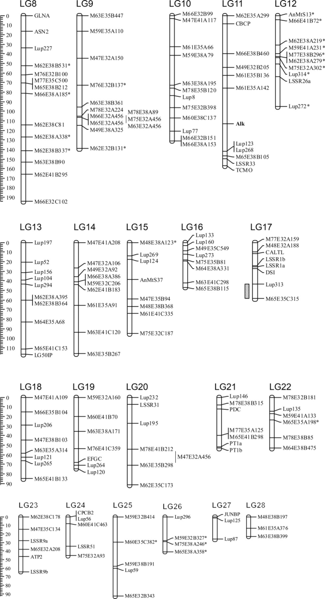
The first genetic linkage map of L. albus. Marker distances in cM are provided on the vertical scale bars. Markers showing distorted segregation are indicated with an asterisk (*). Markers with ambiguous order described by Multipoint v. 1.2 are shown in a second column. Genomic locations of QTLs for flowering time (LG1 and 3) and anthracnose resistance (LG4 and 17) are highlighted to the left of LGs with criss-crossed and diagonally patterned boxes, respectively, and SDs depicted by lines to the sides. Refer to Table 3 for QTL parameters. The locus for alkaloid content on LG11 is indicated in bold.

Overall, 12.8% of markers segregated in a distorted fashion at P < 0.05 and only 4% at P < 0.01. Segregation distortion has been commonly encountered in various plant species such as narrow-leafed lupin (9%),³⁷ chickpea (20.4%),³⁸ and is a common phenomenon in lentil.³⁹ Many factors may be responsible for marker distortion such as structural rearrangement or differences in DNA content, non-random abortion of male and female gametes, and selection for or against a particular allele of one of the parents during propagation of RILs.^40–43

Few of the markers in this study were shared with L. angustifolius, which is partly due to the Kiev Mutant × P27174 cross being relatively narrow. This is evidenced in the number of polymorphic ITAP markers detected, 112/626 for L. albus and 108/424 for L. angustifolius.²³ Of these only 24 were shared in common, and to describe synteny, two or more syntenic markers are required. Only two instances were found with two markers: LG63 and Lup3 (LG1 in L. albus and LG8 in L. angustifolius), and CPCB2 and Lup56 (LG24 in L. albus and LG2 in L. angustifolius). The three extra LGs in L. albus, compared to an expected chromosome number of 25,⁴ seven additional pairs, and 15 unlinked markers might be expected to coalesce and join to the ends of other LGs as more markers are mapped.

3.2. Characteristics of genetic markers

3.2.1. Intron targeted amplified polymorphic sequence

Of the 626 ITAP markers that were screened, 537 amplified in the L. albus genome. Three hundred and seventy-eight of these produced clear single band amplicons (Table 2). From these, 112 polymorphic markers were identified between Kiev Mutant and P27174 (Table 2), of which 105 were used to genotype the 94 individuals of the F8 RIL population (Supplementary Table S1). Chi-squared tests revealed 10 genic markers (about 10%) with distorted segregation (P < 0.05). Of the three genic marker groups, the ‘ML’ markers gave the highest amplification and polymorphism rates (95 and 35%, respectively; Table 2). The ‘MLG’ group amplified with a similar frequency, but fewer amplicons were polymorphic. The ‘MP’ primers amplified at a noticeably lower frequency (60%) but were slightly more polymorphic than the MLG group (Table 2). This data compliments previous studies in Lupinus angustifolius and Lens culinaris,^23,27 and implies an association between the success rates of amplification in the target species based on the phlyogenetic context of primer design, and that primers based on conserved sequences between three species (i.e. MLG primers) may have more conserved introns.

Table 2.

Efficiency of genic markers used to construct the comparative genetic linkage map of L. albus

Marker typea	Screened	Amplificationb (%)	Sequenced	Polymorphismc (%)	Mapped
MP	126	75 (60)	69	14 (20)	14
ML	350	332 (95)	246	87 (35)	81
MLG	150	130 (87)	63	11 (17)	10
Total	626	537	378	112	105

^aPredominant modes of design: MP, markers primarily between M. truncatula and G. Max; ML, between M. truncatula and L. albus; MLG, between M. truncatula, G. Max and L. albus.

^bFigures in parentheses are percentages of amplified markers of the total markers screened.

^cFigures in parentheses are percentages of polymorphic markers of the total markers sequenced.

3.2.2. AFLP markers

One of the most popular molecular marker techniques used for genetic mapping is AFLP.³³ The advantage of AFLPs is their efficiency in simultaneously generating large numbers of molecular markers in a single assay. This technique provides a useful complement to gene-based markers by joining together blocks of genic markers used to identify synteny, as shown between L. angustifolius and M. truncatula.²³

Two hundred and twenty-three discrete markers were generated from 64 selective primer combinations, of which 24 were codominant (i.e. A or B) and 199 dominant (i.e. present or absent). Of these 223 markers, 32 did not segregate in the expected Mendelian ratio of 1:1 (P < 0.05). However, only three of these distorted markers with P < 0.01 were excluded from the map construction process since the remaining markers did not interfere with LG construction.

3.3. L. albus comparative mapping with M. truncatula

To assess the level of synteny between L. albus and M. truncatula, the L. albus genetic map was compared to the most up-to-date version of the M. truncatula physical map. Forty-five of 97 (46%) orthologous markers that have been mapped in M. truncatula revealed evidence of conserved gene order between M. truncatula and L. albus. As shown in Fig. 2, there are numerous breaks in synteny between the two genomes that would be expected given the wide evolutionary distance and difference in chromosome number between the two species (M. truncatula, n = 8; L. albus, n = 25). The orthologous markers identified 17 small syntenic blocks of two or more markers on 17 separate LGs. The remaining 52 markers showed no evidence of macrosynteny, and 15 were unlinked.

Figure 2.

Evidence of macrosynteny between L. albus and M. truncatula genomes. The L. albus LGs are shown in black and the medicago LGs are shown in grey. Orthologous markers joining L. albus and M. truncatula LGs are indicated by broken lines. Distances for M. truncatula markers are provided in cM.

These results imply genome fragmentation, or duplication followed by divergence and selective loss of chromosomes. This would break down lengthy stretches of syntenic chromosome segments observed between closely related legumes, such as those detected between M. truncatula and L. culinaris,²⁷ M. truncatula and M. sativa,³⁰ and M. sativa and Pisum sativum.²¹ Frequently, two or more loci originating from different L. albus LGs were syntenic with a common M. truncatula chromosome. This supports a hypothesis of polyploidization followed by rearrangements, and gene divergence or selective loss of genes and chromosomal fragments. Macrosynteny restricted only to small genomic intervals was also observed between L. angustifolius and M. truncatula,²³ where only 95 of 181 common markers between the two genomes were mapped into 11 small conserved regions, and has been reported in other comparative studies between distantly related legumes such as M. truncatula and soybean.²²

Each of the eight M. truncatula chromosomes showed corresponding syntenic regions in L. albus, with the exception of chromosome 6. This augments previous results between L. angustifolius and M. truncatula,²³ and between M. truncatula and more closely related legume species.²⁰ Chromosome 6 is the smallest M. truncatula chromosome, contains few conserved genes,²⁰ a large proportion of resistance genes,⁴⁴ and is responsible for the different chromosome numbers between M. truncatula and field pea (P. sativum),^21,30 and between M. truncatula and chickpea (Cicer arietinum).²²

3.4. Segregation of agronomic traits

One hundred and ninety-one F8 RILs were phenotyped for anthracnose resistance, alkaloid content, and flowering time. The phenotypic distribution of the anthracnose resistance and flowering time were continuous suggesting that these traits were quantitatively inherited (W > 0.05). ANOVA indicated genetic variation between the recombination inbred lines (r² = 0.89, P < 0.001 for anthracnose resistance and r² = 0.76 with P < 0.0001 for flowering time). The means of disease scores and flowering time for parental lines and the F8 population are shown in Fig. 3.

Figure 3.

Frequency distribution of disease scores for anthracnose resistance (A) and flowering time (B) in 195 L. albus F8 RILs developed from Kiev Mutant and P27174. Three replicates were conducted. The mean disease scores of the anthracnose resistant and susceptible parents are indicated by the letters S and R, respectively. The mean scores of flowering time of the parents are indicated with black arrows. The mean scores of disease and flowering time for all F8 RILs are indicated with white arrows.

Two methods (Dragendorff and UV) were used to determine alkaloid content. The segregation ratio among the RILs was similar in both the methods (89:94 and 88:91, low alkaloid:high alkaloid content, using the Dragendorff and U/V tests, respectively. 1:1, P < 0.05) This suggested a single gene controls alkaloid content. The scores from the two tests were highly correlated (r = 0.85, P = 0.00001, for n = 192).

3.5. QTL mapping of anthracnose resistance

The frequency distribution of anthracnose disease resistance scores in L. albus was continuous implying polygenic control. Interval mapping conducted with MultiQTL software detected two regions significantly associated with anthracnose resistance on LG4 and LG17 at an LOD > 3 (Fig. 1). These QTLs explain over 31 and 26% of the phenotypic variance, respectively, and were inherited from the resistant parent P27174. ANOVA also revealed significant correlation with resistance of two flanking markers (Lup241 and M47E35A209) on LG4 (P < 0.0018 and P < 0.0004, respectively) and two others (Lup313 and M65E35C315 both with P < 0.0001) on LG17. No epistatic interactions were identified between QTLs and unlinked markers using the interactions function in Map Manager QTX. The major QTL on LG17 and a second on LG4 conferring resistance contrasts with L. angustifolius, where a single gene was found to be responsible.³⁷

3.6. QTL mapping of flowering time

Flowering is an important stage in plant development that initiates grain production and is sensitive to stress. The frequency distribution of flowering time was normal in this study, consistent with the polygenic control of this trait observed in other crops. In Arabidopsis, seven QTLs were detected controlling flowering time,⁴⁵ while in chickpea and soybean, two and four QTLs were identified, respectively.^46,47 This result in L. albus contrasts with previous mapping studies in L. angustifolius where flowering time was controlled by a major gene, Ku²³.

Two significant QTLs at the top of LG1 and LG3 at a LOD score of > 3 were detected using interval mapping (Fig. 1; Table 3), which together explain more than 52% of the total phenotypic variation. The strongest QTL, explaining 31% of the phenotypic variance at the top of LG3, covered a relatively wide distance of ∼10 cM. Due to population size and/or the number of recombinants in a particular region, interval mapping usually underestimates or is unable to identify the number of genes conditioning quantitative traits. Therefore two or more QTLs may be detected as a single QTL in small populations (<500 individuals) if closer together than ∼20 cM.^48,49

Table 3.

Estimates of QTLs determined using MultiQTL with significant effects on anthracnose resistance and flowering time in L. albus Kiev Mutant x P₂₇₁₇₄ F8 RILs

QTL estimatesa	Anthracnose resistance		Flowering time
LG [interval]b	4 [9]	17 [6]	1 [1]	3 [1 and 2]
Pc	0.012	0.000***	0.002**	0.000***
LODd	5.58 (1.01)	5.68 (1.7)	4.76 (1.06)	7.35 (1.98)
Positione	67.3 (38.4)	51.9 (6.02)	1.35 (9.4)	10.7 (8.73)
PEVf	0.31 (11.7)	0.26 (0.07)	0.21 (0.04)	0.31 (0.07)
Response meang	3.26 (0.08)	3.18 (0.08)	3.5 (0.07)	3.5 (0.05)
Effecth	−0.95 (0.18)	−0.86 (0.13)	0.69 (0.09)	0.81 (0.17)
Linked/flanking markers	Lup241M47E35A209	Lup313M65E35C315	M61E32B396	M47E32A266M75E38A83M75E38B73

^aSDs are shown in parentheses.

^bLG and interval within LG associated with the quantitative trait.

^cProbability values from 1000 permutation tests. Asterisks indicate genome-wide significance for false discovery rate: 10 (*), 5 (**), and 1% (***).

^d–hEstimated by 1000 bootstrap tests.

^dMaximum LOD score for a given interval.

^ePosition (cM) of maximum LOD value measured from the first marker in corresponding LG (0 cM).

^fProportion of explained variability by the putative QTL.

^gMeans of anthracnose resistance and flowering time.

^hEffects of the QTLs on the response of anthracnose resistance and flowering time.

The second QTL for flowering time at the top of LG1 explained 21% of the phenotypic variation observed. In the present map, three AFLP markers (M61E32B396, M75E38A83, M75E38B73) cosegregate with the QTL at the end of the LG, suggesting that more markers will be needed to extend this LG to more precisely define the locus.

A third QTL was identified on LG12 that accounted for 11% of the trait at an LOD = 2.4. However, Map Manager QTX did not support this QTL (data not shown). Single-point analysis showed four linked and/or flanking markers (M61E32B396 on LG1 and M47E32A266, M75E38A83, M75E38B73 on LG3) significantly associated with flowering time (P < 0.001). Markers M61E32B396 and M75E38B73 were inherited from Kiev Mutant, whereas M47E32A266 and M75E38A83 were from P27174. No epistatic interactions were detected between these QTLs or unlinked markers using the interactions function in Map Manager QTX.

3.7. Genetic mapping of alkaloid content

A single locus determining alkaloid content mapped to LG11, flanked by markers M61E35A142 and Lup123 (Fig. 1). These results are consistent with the earlier results that Kiev Mutant has a single gene (pauper) for low alkaloid content.⁵⁰ In L. angustifolius, alkaloid content was also found to be controlled by a single locus.²³ Interestingly, Lup268 which flanks the QTL in L. albus, mapped to a separate chromosome to alkaloid content in L. angustifolius. This suggests either these two loci are independent or there has been rearrangement between the lupin genomes.

3.8. Future prospects for the application of synteny in L. albus

While synteny between L. albus and M. truncatula in this study was limited to small conserved blocks of genes, these may help in identifying more closely linked markers or candidate genes if desirable traits map to such regions. Where structural differences exist between more distantly related species such as M. truncatula and soybean, it is notable that significant microsynteny, or conservation at the DNA sequence level, exists.⁵¹ Thus one would expect progress in the application of both macro- and microsynteny to identify closely linked markers and to isolate important genes; precedents in other families include the Solanaceae,⁵² Poaceae,^53–55 and Rosaceae.⁵⁶

Although the L. albus genetic and comparative map comprised more than 300 markers, there were not enough shared markers to make a detailed comparison of the L. albus and L. angustifolius genomes, as this is the most obvious way to investigate Genistoid evolution. More markers are also needed to consolidate the number of chromosomes and increase marker density. The present study provides markers associated with anthracnose and flowering QTLs that were significantly associated with these traits. More tightly linked molecular markers are required, however, for efficient marker-assisted selection in breeding programs involving these parental lines. Nevertheless, this research throws light on the processes of chromosomal evolution in the Genistoid clade, is the first report on the genetic mapping of economically important traits in L. albus, and forms the basis of a resource for the L. albus and legume research community.

Supplementary data

Supplementary data are available online at www.dnaresearch.oxfordjournals.org.

References

- 1.Langridge D. F., Goodman R. D. Honeybee pollination of lupins (Lupinus albus cv.Hamburg) Aust. J. Expt. Agric. 1985;25:220–223. [Google Scholar]
- 2.Payne W. A., Chen C., Ball D. A. Agronomic potential of narrow-leafed and white lupins in the inland Pacific northwest. Agron J. 2004;96:1501–1508. [Google Scholar]
- 3.Pazy B., Heyn C., Herrnstadt I., Plitmann U. Studies in populations of the Old World Lupinus species. I. Chromosomes of the East-Mediterranean lupines. Israel J. Bot. 1977;26:115–127. [Google Scholar]
- 4.Naganowska B., Wolko B., Sliwinska E., Kaczmarek Z. Nuclear DNA content variation and species relationships in the genus Lupinus (Fabaceae) Ann. Bot. 2003;92:349–355. doi: 10.1093/aob/mcg145. [DOI] [PMC free article] [PubMed] [Google Scholar]
- 5.Lindbeck K. D., Murray G. M., Priest M., Dominiak B. C., Nikandrow A. Survey for anthracnose caused by Colletotrichum gloeosporioides in crop lupins (Lupinus angustifolius, L. albus) and ornamental lupins (L. polyphyllus) in New South Wales. Australasian Plant Pathology. 2001;27:259–262. [Google Scholar]
- 6.Noffsinger S.L., van Santen E. Evaluation of Lupinus albus L. Germplasm for the Southeastern USA. Crop Sci. 2005;45:1941–1950. [Google Scholar]
- 7.Uauy R., Gattas V., Yanez E. In: World Review of Nutrition and Dietetics. Simopoulos A. M., editor. Vol. 77. Karger, Basel; 1995. pp. 75–88. [DOI] [PubMed] [Google Scholar]
- 8.Hall R. S., Johnson S. K., Baxter A. L., Ball M. J. Lupin kernel fibre-enriched foods beneficially modify serum lipids in men. Eur. J. Clin. Nutr. 2004;59:325–333. doi: 10.1038/sj.ejcn.1602077. [DOI] [PubMed] [Google Scholar]
- 9.Edwards A. C., van Barneveld R. J. In: Lupins as Crop Plants: Biology, Production and Utilization. Gladstones J. S., Atkins C., Hamblin J., editors. Wallingford: CAB International; 1998. pp. 385–410. [Google Scholar]
- 10.Hamama A. A., Bhardwaj H. L. Phytosterols, triterpene alcohols, and phospholipids in seed oil from white lupin. J. Am. Oil Chem. Soc. 2004;81:1039–1044. [Google Scholar]
- 11.Dinkelaker B., Romheld V., Marschner H. Citric acid excretion and precipitation of calcium citrate in the rhizosphere of white lupin (Lupinus albus L.) Plant Cell Environ. 1989;12:285–292. [Google Scholar]
- 12.Gardner W. K., Parbery D. G., Barber D. A. The acquisition of phosphorus by Lupinus albus L. I. Some characteristics of the soil/root interface. Plant Soil. 1982;68:19–32. [Google Scholar]
- 13.Johnson J. F., Vance C. P., Allan D. L. Phosphorus deficiency in Lupinus albus (altered lateral root development and enhanced expression of phosphoenolpyruvate carboxylase) Plant Physiol. 1996;112:31–41. doi: 10.1104/pp.112.1.31. [DOI] [PMC free article] [PubMed] [Google Scholar]
- 14.Massonneau A., Langlade N., Léon S., et al. Metabolic changes associated with cluster root development in white lupin (Lupinus albus L.): relationship between organic acid excretion, sucrose metabolism and energy status. Planta. 2001;213:534–542. doi: 10.1007/s004250100529. [DOI] [PubMed] [Google Scholar]
- 15.Neumann G., Martinoia E. Cluster roots—an underground adaptation for survival in extreme environments. Trends Plant Sci. 2002;7:162–167. doi: 10.1016/s1360-1385(02)02241-0. [DOI] [PubMed] [Google Scholar]
- 16.Devos K. M., Gale M. D. Genome relationships: the grass model in current research. Plant Cell. 2000;12:637–646. doi: 10.1105/tpc.12.5.637. [DOI] [PMC free article] [PubMed] [Google Scholar]
- 17.Lagercrantz U., Lydiate D. J. Comparative genome mapping in Brassica. Genetics. 1996;144:1903–1910. doi: 10.1093/genetics/144.4.1903. [DOI] [PMC free article] [PubMed] [Google Scholar]
- 18.Moore G., Devos K. M., Wang Z., Gale M. D. Cereal genome evolution—grasses, line up and form a circle. Curr. Biol. 1995;5:737–739. doi: 10.1016/s0960-9822(95)00148-5. [DOI] [PubMed] [Google Scholar]
- 19.Ventelon M., Deu M., Garsmeur O., et al. A direct comparison between the genetic maps of sorghum and rice. Theor. Appl. Genet. 2001;102:379–386. [Google Scholar]
- 20.Choi H.-K., Mun J.-H., Kim D.-J., et al. Estimating genome conservation between crop and model legume species. PNAS. 2004;101:15289–15294. doi: 10.1073/pnas.0402251101. [DOI] [PMC free article] [PubMed] [Google Scholar]
- 21.Kalo P., Seres A., Taylor S., et al. Comparative mapping between Medicago sativa and Pisum sativum. Mol. Genet. Genomics. 2004;272:235–246. doi: 10.1007/s00438-004-1055-z. [DOI] [PubMed] [Google Scholar]
- 22.Zhu H., Choi H.-K., Cook D. R., Shoemaker R. C. Bridging model and crop legumes through comparative genomics. Plant Physiol. 2005;137:1189–1196. doi: 10.1104/pp.104.058891. [DOI] [PMC free article] [PubMed] [Google Scholar]
- 23.Nelson M., Phan H., Ellwood S., et al. The first gene-based map of Lupinus angustifolius L.-location of domestication genes and conserved synteny with Medicago truncatula. Theor. Appl. Genet. 2006;113:225–238. doi: 10.1007/s00122-006-0288-0. [DOI] [PubMed] [Google Scholar]
- 24.Phan H. T. T., Ellwood S. R., Ford R., Thomas S., Oliver R. Differences in syntenic complexity between Medicago truncatula with Lens culinaris and Lupinus albus. Funct. Plant Biol. 2006;33:775–782. doi: 10.1071/FP06102. [DOI] [PubMed] [Google Scholar]
- 25.Lukens L., Zou F., Lydiate D., Parkin I., Osborn T. Comparison of a Brassica oleracea genetic map with the genome of Arabidopsis thaliana. Genetics. 2003;164:359–372. doi: 10.1093/genetics/164.1.359. [DOI] [PMC free article] [PubMed] [Google Scholar]
- 26.Weeden N. F., Muehlbauer F. J., Ladizinsky G. Extensive conservation of linkage relationships between pea and lentil genetic maps. J. Hered. 1992;83:123–129. [Google Scholar]
- 27.Phan H. T. T., Ellwood S. R., Hane J. K., Ford R., Materne M., Oliver R. P. Extensive macrosynteny between Medicago truncatula and Lens culinaris ssp. culinaris. Theor. Appl. Genet. 2007;114:549–558. doi: 10.1007/s00122-006-0455-3. [DOI] [PubMed] [Google Scholar]
- 28.Aubert G., Morin J., Jacquin F., et al. Functional mapping in pea, as an aid to the candidate gene selection and for investigating synteny with the model legume Medicago truncatula. Theor. Appl. Genet. 2006;112:1024–1041. doi: 10.1007/s00122-005-0205-y. [DOI] [PubMed] [Google Scholar]
- 29.Choi H. K., Luckow M. A., Doyle J., Cook D. R. Development of nuclear gene-derived molecular markers linked to legume genetic maps. Mol. Genet. Genomics. 2006;276:56–70. doi: 10.1007/s00438-006-0118-8. [DOI] [PubMed] [Google Scholar]
- 30.Choi H.-K., Kim D., Uhm T., et al. A sequence-based genetic map of Medicago truncatula and comparison of marker colinearity with M. sativa. Genetics. 2004;166:1463–1502. doi: 10.1534/genetics.166.3.1463. [DOI] [PMC free article] [PubMed] [Google Scholar]
- 31.Eujayl I., Sledge M., Wang L., et al. Medicago truncatula EST-SSRs reveal cross-species genetic markers for Medicago spp. Theor. Appl. Genet. 2004;108:414–422. doi: 10.1007/s00122-003-1450-6. [DOI] [PubMed] [Google Scholar]
- 32.Gutierrez M. V., Vaz Patto M. C., Huguet T., Cubero J. I., Moreno M. T., Torres A. M. Cross-species amplification of Medicago truncatula microsatellites across three major pulse crops. Theor. Appl. Genet. 2005;110:1210–1217. doi: 10.1007/s00122-005-1951-6. [DOI] [PubMed] [Google Scholar]
- 33.Vos P., Hogers R., Bleeker M., et al. AFLP: a new technique for DNA fingerprinting. Nucl. Acids Res. 1995;23:4407–4414. doi: 10.1093/nar/23.21.4407. [DOI] [PMC free article] [PubMed] [Google Scholar]
- 34.Ellwood S. R., D'Souza N. K., Kamphuis L. G., Burgess T. I., Nair R. M., Oliver R. P. SSR analysis of the Medicago truncatula SARDI core collection reveals substantial diversity and unusual genotype dispersal throughout the Mediterranean basin. Theor. Appl. Genet. 2006;112:977–983. doi: 10.1007/s00122-005-0202-1. [DOI] [PubMed] [Google Scholar]
- 35.Manly K. F., Cudmore R. H., Meer J. M. Map Manager QTX, cross-platform software for genetic mapping. Mamm. Genome. 2001;12:930–932. doi: 10.1007/s00335-001-1016-3. [DOI] [PubMed] [Google Scholar]
- 36.King G. J. Through a genome, darkly: comparative analysis of plant chromosomal DNA. Plant Mol. Biol. 2002;48:5–20. [PubMed] [Google Scholar]
- 37.Boersma J. G., Pallotta M., Li C., Buirchell B. J., Sivasithamparam K., Yang H. Construction of a genetic linkage map using MFLP and identification of molecular markers linked to domestication genes in narrow-leafed lupin (Lupinus angustifolius L.) Cell. Mol. Biol. Lett. 2005;10:331–344. [PubMed] [Google Scholar]
- 38.Flandez-Galvez H., Ford R., Pang E. C. K., Taylor P. W. J. An intraspecific linkage map of the chickpea (Cicer arietinum L.) genome based on sequence tagged microsatellite site and resistance gene analog markers. Theor. Appl. Genet. 2003;106:1447–1456. doi: 10.1007/s00122-003-1199-y. [DOI] [PubMed] [Google Scholar]
- 39.Muehlbauer F. J., Cho S., Sarker A., et al. Application of biotechnology in breeding lentil for resistance to biotic and abiotic stress. Euphytica. 2006;147:149–165. [Google Scholar]
- 40.Paran I., Goldman I., Tanksley S. D., Zamir D. Recombinant inbred lines for genetic mapping in tomato. Theor. Appl. Genet. 1995;90:542–548. doi: 10.1007/BF00222001. [DOI] [PubMed] [Google Scholar]
- 41.Quillet M. C., Madjidian N., Griveau Y., et al. Mapping genetic factors controlling pollen viability in an interspecific cross in Helianthus sect. Helianthus. Theor. Appl. Genet. 1995;91:1195–1202. doi: 10.1007/BF00220929. [DOI] [PubMed] [Google Scholar]
- 42.Tadmor Y., Zamir D., Ladizinsky G. Genetic mapping of an ancient translocation in the genus Lens. Theor. Appl. Genet. 1987;73:883–892. doi: 10.1007/BF00289394. [DOI] [PubMed] [Google Scholar]
- 43.Xu Y., Zhu L., Xiao J., Huang N., McCouch S. R. Chromosomal regions associated with segregation distortion of molecular markers in F2, backcross, doubled haploid, and recombinant inbred populations in rice (Oryza sativa L.) Mol. Genet. Genomics. 1997;253:535–545. doi: 10.1007/s004380050355. [DOI] [PubMed] [Google Scholar]
- 44.Zhu H., Cannon S. B., Young N. D., Cook D. R. Phylogeny and genomic organization of the TIR and non-TIR NBS-LRR resistance gene family in Medicago truncatula. Mol. Plant Microbe Interact. 2002;15:529–359. doi: 10.1094/MPMI.2002.15.6.529. [DOI] [PubMed] [Google Scholar]
- 45.Kuittinen H., Sillanpaa M. J., Savolainen O. Genetic basis of adaptation: flowering time in Arabidopsis thaliana. Theor. Appl. Genet. 1997;95:573–583. [Google Scholar]
- 46.Lichtenzveig J., Bonfil D. J., Zhang H.-B., Shtienberg D., Abbo S. Mapping quantitative trait loci in chickpea associated with time to flowering and resistance to Didymella rabiei the causal agent of Ascochyta blight. Theor. Appl. Genet. 2006;113:1357–1369. doi: 10.1007/s00122-006-0390-3. [DOI] [PubMed] [Google Scholar]
- 47.Yamanaka N., Ninomiya S., Hoshi M., et al. An informative linkage map of soybean reveals QTLs for flowering time, leaflet morphology and regions of segregation distortion. DNA Res. 2001;8:61–72. doi: 10.1093/dnares/8.2.61. [DOI] [PubMed] [Google Scholar]
- 48.Liu B. H. Statistical Genomics: Linkage, Mapping and QTL Analysis. Boca Raton: CRC Press; 1985. [Google Scholar]
- 49.Tanksley S. D. Mapping polygenes. Annual Review of Genetics. 1993;27:205–233. doi: 10.1146/annurev.ge.27.120193.001225. [DOI] [PubMed] [Google Scholar]
- 50.Harrison J. E. M., Williams W. Genetical control of alkaloids in Lupinus albus. Euphytica. 1982;31:357–364. [Google Scholar]
- 51.Yan H., Mudge J., Kim D., Shoemaker R., Cook D., Young N. Comparative physical mapping reveals features of microsynteny between Glycine max, Medicago truncatula, and Arabidopsis thaliana. Genome. 2004;47:141–155. doi: 10.1139/g03-106. [DOI] [PubMed] [Google Scholar]
- 52.Huang S., van der Vossen E. A., Kuang H., et al. Comparative genomics enabled the isolation of the R3a late blight resistance gene in potato. Plant J. 2005;42:251–261. doi: 10.1111/j.1365-313X.2005.02365.x. [DOI] [PubMed] [Google Scholar]
- 53.Armstead I. P., Skot L., Turner L. B., et al. Identification of perennial ryegrass (Lolium perenne (L.)) and meadow fescue (Festuca pratensis (Huds.)) candidate orthologous sequences to the rice Hd1(Se1) and barley HvCO1 CONSTANS-like genes through comparative mapping and microsynteny. New Phytol. 2005;167:239–247. doi: 10.1111/j.1469-8137.2005.01392.x. [DOI] [PubMed] [Google Scholar]
- 54.Börner A., Korzun V., Worland A. J. Comparative genetic mapping of loci effecting plant height and development in cereals. Euphytica. 1998;100:245–248. [Google Scholar]
- 55.Mammadov J., Steffenson B., Maroof M. High-resolution mapping of the barley leaf rust resistance gene Rph5 using barley expressed sequence tags (ESTs) and synteny with rice. Theor. Appl. Genet. 2005;111:1651–1660. doi: 10.1007/s00122-005-0100-6. [DOI] [PubMed] [Google Scholar]
- 56.Dirlewanger E., Graziano E., Joobeur T., et al. Comparative mapping and marker-assisted selection in Rosaceae fruit crops. PNAS. 2004;101:9891–9896. doi: 10.1073/pnas.0307937101. [DOI] [PMC free article] [PubMed] [Google Scholar]